
Board of Governors of the Federal Reserve System
International Finance Discussion Papers
Number 891, April 2007 --- Screen Reader
Version*
Some Simple Tests of the Globalization and Inflation Hypothesis
NOTE: International Finance Discussion Papers are preliminary materials circulated to stimulate discussion and critical comment. References in publications to International Finance Discussion Papers (other than an acknowledgment that the writer has had access to unpublished material) should be cleared with the author or authors. Recent IFDPs are available on the Web at http://www.federalreserve.gov/pubs/ifdp/. This paper can be downloaded without charge from the Social Science Research Network electronic library at http://www.ssrn.com/.
Abstract:
This paper evaluates the hypothesis that globalization has increased the role of international factors and decreased the role of domestic factors in the inflation process in industrial economies. Toward that end, we estimate standard Phillips curve inflation equations for 11 industrial countries and use these estimates to test several predictions of the globalization and inflation hypothesis. Our results provide little support for that hypothesis. First, the estimated effect of foreign output gaps on domestic consumer price inflation is generally insignificant and often of the wrong sign. Second, we find no evidence that the trend decline in the sensitivity of inflation to the domestic output gap observed in many countries owes to globalization. Finally, and most surprisingly, our econometric results indicate no increase over time in the responsiveness of inflation to import prices for most countries. However, even though we find no evidence that globalization is affecting the parameters of the inflation process, globalization may be helping to stabilize real GDP and hence inflation. Over time, the volatility of real GDP growth has declined by more than the volatility of domestic demand, suggesting that net exports increasingly are acting to buffer output from fluctuations in domestic demand.
Keywords: inflation, globalization, Phillips curve
JEL classification: C22, E31, F41
I. Introduction
The past several years have seen a sharp escalation of interest in globalization and its effects on all aspects of economic life. There is no single definition of globalization, but most observers define it as the increasing international integration of national markets, including for goods, services, capital, and labor (Frankel, 2006). Among the areas where globalization is thought, at least by some, to be exerting increasing influence is the behavior of inflation.
In the standard view, inflation is characterized primarily as a function of domestic factors such as aggregate demand, wage behavior, productivity, inflation expectations and, influencing the balance between all of these factors, national monetary policy. Of course, some external shocks, such as to import and energy prices, are also thought to affect inflation, but perhaps to a less fundamental extent. More recently, some observers have suggested that globalization is diminishing the role of domestic factors in the inflation process and elevating the role of global developments. Such a shift, as one observer puts it provocatively, ``makes a nonsense of traditional closed-economy models used to forecast inflation, which assume that firms set prices by adding a mark-up over unit costs, with the size of the margin depending on the amount of slack in the economy'' (The Economist, September 14, 2006).
The extent to which globalization has replaced domestic with international factors as a primary determinant of inflation is the subject of active debate. Borio and Filardo (2006) argue that ``the relevance of a more `globe-centric' approach is likely to have increased as the process of integration of the world economy has gathered momentum, a process commonly referred to as `globalization'. (Page 1) In contrast, Ball (2006) writes ``there is little reason to think that globalization has changed the structure of the Phillips curve or the long-run level of inflation'' (Page 15).
Not surprisingly, monetary policymakers have taken an active interest in the topic of globalization and inflation. Federal Reserve Board Chairman Ben Bernanke notes that although globalization has not ``led to significant changes in the process that determines the U.S. inflation rate... effective monetary policy making now requires taking into account a diverse set of global influences, many of which are not fully understood'' (Bernanke, 2007). Federal Reserve Bank of Dallas President Richard Fisher has argued that ``the old models simply no longer apply in our globalized, interconnected and expanded economy... By spurring productivity and fomenting tectonic economic changes, globalization has acted as a tailwind for the Fed's--and other central banks--efforts to hold down inflation'' (Fisher, 2006).1 This sentiment is echoed in a recent statement by Lucas Papademos, Vice President of the European Central Bank: ``One conclusion that has some empirical support is that domestic inflation is no longer determined predominantly by domestic demand and supply constraints, but seems to depend more on the degree of global economic slack'' (2006, page 6). Donald Kohn, Vice Chairman of the Federal Reserve Board, and Janet Yellen, President of the Federal Reserve Bank of San Francisco, acknowledge that international forces likely are playing an increasingly important role in the inflation process, but conclude that domestic considerations probably retain a predominant role (Kohn, 2006, Yellen, 2006).
One of the factors keeping the debate over globalization and inflation alive is the absence of a wide range of compelling and consistent empirical evidence. There has not been a great deal of research on this topic, and what research there has been comes up with conflicting findings. This paper contributes to the discussion on globalization and inflation in two ways. First, we present a comprehensive evaluation of the major channels through which globalization may have changed the dynamics of inflation formation. More specifically, we use Phillips curve equations, estimated over the period 1977-2005 for 11 OECD economies, to assess three major implications of the globalization and inflation hypothesis: (1) measures of foreign resource utilization are affecting domestic inflation, and to an increasing extent over time; (2) by the same token, domestic inflation is becoming less sensitive to domestic resource utilization, reflecting increased economic openness, and (3) domestic inflation is becoming increasingly sensitive to import prices. Secondly, in our research, we eschew complicated econometric specifications in favor of standard, straightforward, and transparent inflation models. This makes it less likely that particular findings will owe to the particular econometric specification used.
Before proceeding, several initial considerations should be addressed. First, all papers on this topic generally acknowledge that in the long run the rate of inflation is set by domestic monetary policy. Accordingly, the argument that globalization has affected the inflation process is an argument that applies in the short to medium term, when shocks to prices or resource utilization beyond a country's borders may temporarily influence a country's domestic inflation rate. The resultant deviations of inflation from the monetary authorities' desired rate should induce monetary policy actions designed to return inflation to that desired rate over the longer run. Moreover, the stance of monetary policy, by influencing the behavior of inflation expectations, may also affect how much inflation responds to shocks in the nearer term and how quickly it recovers.2
Of course, some have argued that monetary authorities have been willing to accommodate positive supply shocks, such as falling import prices, over time as they have pursued a strategy of ``opportunistic disinflation'' (See Orphanides and Wilcox, 2002). In the context of such a strategy, foreign shocks that depress inflation arguably may have a persistent effect as long as inflation exceeds the central bank's long-term objective. Also, Rogoff (2003) argues that deregulation and international integration have led to more flexible prices, so that inflation surprises induced by monetary policy lead to more inflation and less additional activity than in the past. Accordingly, in Rogoff's argument globalization has led monetary authorities to target lower inflation rates.3
Second, and as a related point, what allows the monetary authority to unilaterally control the domestic inflation rate over the longer term is a floating exchange rate. With fixed exchange rates, a country necessarily will import both foreign inflationary conditions and, with sufficient capital mobility, foreign monetary policy as well. Floating exchange rates, in contrast, allow the monetary authority to set interest rates independently of those abroad. Moreover, as stressed by Kohn (2006) and Yellen (2006), floating exchange rates insert a wedge between movements in foreign prices and movements in the domestic-currency prices of products imported from abroad. Thus, even if foreign economies are booming and foreign price pressures are building, this need not lead to price pressures domestically if the domestic currency is rising against foreign currencies.
Finally, the topic of globalization and inflation embraces two broad sets of questions. The first, which is the subject of this paper, is whether globalization has changed the parameters of the inflation process, so that domestic inflation is now more sensitive to events beyond a country's borders and less sensitive to domestic events. The second issue is whether globalization has led recently to a decline in the inflation rates of industrial economies, in particular because of the integration of low-wage, low-cost countries-e.g., China, India, Eastern Europe-into the global economy. China and other low-wage economies may have depressed industrial-country inflation both directly, by reducing import prices, and perhaps also indirectly, by influencing the process of wage and price formation in the industrialized nations.4In any event, quantifying this ``China effect'' involves different sets of issues and data than analyzing the impact of globalization more generally on the behavior and dynamics of inflation. 5
Therefore, to keep our research project focused, we confine ourselves to assessing the evidence on how globalization in general has altered the inflationary process. The plan of this paper is as follows. Section II describes the ``globalization and inflation'' hypothesis in greater detail. Section III assesses the hypothesis that foreign resource utilization is becoming more important to domestic inflation. Section IV explores whether the flattening of the Phillips Curve owes to globalization, and Section V assesses whether, for the same reason, domestic inflation is becoming more sensitive to import prices. Section VI addresses the stabilizing effect of net exports as a possible consequence of globalization. Section VII concludes.
II. The Logic of the Globalization and Inflation Hypothesis
The premise that globalization is affecting the dynamics of the inflation process rests on the view that, with national markets increasingly integrated with each other, prices of goods, services, labor, and capital increasingly can be arbitraged across national borders. In consequence, rather than being set exclusively by domestic supply/demand conditions within a given country, prices of products and factor inputs are now influenced by supply/demand conditions in global markets.
Equation (1), below, represents a very stylized Phillips curve model of inflation, with inflation depending on inflation expectations, the domestic (i.e., home country) output gap, and a supply shock, the deviation of import price inflation from expected CPI inflation.6 This equation has the feature that consumer price inflation equals expected inflation when the economy is operating at capacity and import price inflation moves in line with consumer price inflation.7 The globalization and inflation hypothesis has at least three implications for the inflation process as summarized in this model.
![]() YGAP +
YGAP +
![]() -
- ![]() (1)
(1)
![]() : CPI inflation
: CPI inflation
![]() : CPI inflation expectations
: CPI inflation expectations
![]() : import price inflation
: import price inflation
YGAP : output gap (actual output relative to potential)
First, and most obviously, as economies become more open and
more integrated with each other, it is logical that the direct
sensitivity of domestic inflation to movements in import
prices--represented by ![]() in equation (1)-should
increase. This may reflect increases in the direct effect of import
prices on the CPI, as the share of imports in consumption rises. It
may also reflect increasing indirect effects of import prices as
the share of imports in intermediate inputs rise, or as increasing
import penetration and competition lead to closer pricing of
similar categories of domestic and imported goods.
in equation (1)-should
increase. This may reflect increases in the direct effect of import
prices on the CPI, as the share of imports in consumption rises. It
may also reflect increasing indirect effects of import prices as
the share of imports in intermediate inputs rise, or as increasing
import penetration and competition lead to closer pricing of
similar categories of domestic and imported goods.
Second, some argue that if the globalization and inflation hypothesis is correct, the standard model must be further augmented by a term representing the extent of resource utilization in foreign economies. This is indicated in equation (2), below. The extent of global slack is posited to influence the extent of global inflation, which in turn affects domestic inflation. Moreover, the effect of foreign resource utilization on domestic inflation could operate through factor markets as well as product markets: If domestic wages rise too quickly, for example, this is more likely to lead to domestic production cuts, the offshoring of jobs, and/or a moderation of wage and price pressures when foreign labor markets are loose than when they are tight.
![]() YGAP +
YGAP + ![]() YGAP
YGAP
![]() (2)
(2)
YGAP![]() : Foreign output gap (actual output
relative to potential)
: Foreign output gap (actual output
relative to potential)
Third, and by the same token, some reason that as globalization
proceeds and global slack becomes more important to domestic
inflation, measures of domestic resource utilization must become
relatively less important in determining domestic inflation. That
is, ![]() in equation (2) should decline.8
in equation (2) should decline.8
Some may protest that in an inflation model that incorporates import prices, those import prices already encompass the behavior of foreign resource utilization, and there is no scope for a separate variable capturing global slack to influence domestic prices. However, as Borio and Filardo (2006) point out, import prices are not a ``sufficient statistic'' for the influence of foreign markets on domestic prices. To begin with, import prices capture only the cost of goods and services that are actually imported; they do not capture the cost of other products that potentially could be imported if domestic prices rise too far above their foreign counterparts. (It is often suggested that the mere threat of foreign competition may keep domestic prices--and wages--in check.) Additionally, because many domestic firms sell their products both in the domestic and foreign markets, the prices they charge in domestic markets are likely to be influenced by the prices they can charge in foreign markets; it is not clear how correlated those latter prices will be with import prices. And, as noted above, the effect of foreign resource utilization on domestic inflation may operate through factor markets, wage differentials, and the threat of offshoring rather than through import prices alone.
There are several additional hypothesis for how globalization may have altered the inflation process, although they are not well supported by the data. First, some observers suggest that increases in trade openness have led to increased competition and hence reduced markups of price over cost (Chen, Imbs, and Scott, 2004). However, as pointed out by Kohn (2006), the rise in profit rates in recent years is inconsistent with the view that markups have declined.
Second, and as a related point, some speculate that increased trade, by exposing domestic producers to foreign competition, has boosted productivity growth, and this could explain the downshifts in inflation that occurred around the world in the 1990s. This contention, too, is not well supported by the facts. Although U.S. productivity accelerated in the 1990s, many other industrial economies where trade openness rose experienced no corresponding rise in productivity growth.9
III. The Role of Foreign Output Gaps
This and the following two sections describe research to test the three predictions of the globalization and inflation hypothesis described above: that globalization has increased the role of foreign output gaps in determining inflation, that it has reduced the role of domestic output gaps, and that it has increased the sensitivity of inflation to import prices. In this section, we address the first of these predictions. We begin by describing previous research on this topic, and then present our own results.
III.1 Previous research
Tootell (1998) estimates a standard Phillips curve model for the United States over the 1973-1996 period and adds to the model trade-weighted measures of foreign resource utilization-both unemployment and the output gap-for six U.S. trading partners; he finds no evidence that these measures affect U.S. inflation. Gamber and Hung (2001) also estimate a Phillips curve model for the United States over a similar period, 1976-1999. In contrast to Tootell, they find that a trade-weighted average of capacity utilization for 35 U.S. trading partners positively and significantly affects U.S. inflation. Wynne and Kersting (2007) also find some support for the role of foreign resource utilization both when they extend Tootell's model to the present, and when they examine the correlation of foreign output gaps with detrended U.S. inflation. However, Hooper, Slok, and Dobridge (2006) find that the aggregate output gap for the OECD does not help explain U.S. inflation.
The strongest and broadest results for the role of foreign resource utilization are in Borio and Filardo (2006). They estimate Phillips curve models for 16 OECD countries (plus the euro area) over 1985-2005. Both in equations for individual countries and for a time-series/cross-country panel, they find the effect of weighted-average foreign output gaps on domestic inflation to be positive and highly significant, to generally exceed the effect of domestic output gaps, and to be rising over time. These results are robust to the inclusion of additional explanatory variables, including import prices and unit labor costs.
However, other recent efforts to evaluate the role of foreign resource utilization in a cross-country setting have not identified significant effects. Pain, Koske, and Sollie (2006) find no role for a global output gap in inflation equations for 21 OECD countries estimated over 1980-2005. Ball (2006), estimating a panel regression for 14 OECD countries over 1985-2005, finds the effect of the foreign output gap on domestic inflation to be smaller than that of the domestic output gap, to be of only marginal significance, and to add little explanatory power.
III.2 New results
Because Borio and Filardo (2006) report results that strongly support the role of foreign resource utilization, and because those results have received widespread attention, we start by describing their methodology and we then assess the robustness of their results to alternative specifications of the inflation equation.
Equation (3) below reproduces the Borio-Filardo paper's simplest equation, a regression of de-trended four-quarter inflation in a given country on a constant and that country's output gap. Equation (4) adds as an explanatory variable a weighted average of the output gap in that country's trading partners.
![\begin{displaymath} \begin{array}[c]{l} (3)\text{ }\pi_{4t}-\pi_{4t}^{e}=\alpha+\delta\cdot Y_{t-1}\ \ (4)\text{ }\pi_{_{4t}}-\pi_{4t}^{e}=\alpha+\delta\cdot Y_{t-1}+\gamma\cdot Y_{t-1}^{\ast},\ \end{array}\end{displaymath}](img13.gif)
![\begin{displaymath} \begin{array}[c]{l} \pi_{4t}=\left( {\frac{CPI_{t}^{headline}-CPI_{t-4}^{headline}} {CPI_{t-4}^{headline}}}\right) \ast100\ \ \pi_{4t}^{e}=HP\left( {(\frac{CPI_{t}^{core}-CPI_{t-4}^{core}}{CPI_{t-4} ^{core}})\ast100}\right) ,\ \end{array}\end{displaymath}](img14.gif)
and where
![]() is the headline CPI,
is the headline CPI,
![]() is the CPI excluding food and
energy,
is the CPI excluding food and
energy, ![]() is the domestic output gap (actual
relative to potential),
is the domestic output gap (actual
relative to potential),
![]() is the foreign output gap (actual
relative to potential), and
is the foreign output gap (actual
relative to potential), and ![]() is an HP-filter
of variable
is an HP-filter
of variable ![]() .
.
The definition of the dependent variable--headline consumer price inflation minus trend core inflation--is unusual. The Borio-Filardo paper motivates this specification by suggesting that trend core inflation may proxy for inflation expectations. In order to assess the robustness of the Borio-Filardo results to changes in econometric specification, it is important to first be able to reproduce their benchmark estimates for a broad range of industrial economies. We do so for 14 industrial economies, drawing on most of the same data sources as the Borio-Filardo paper: inflation rates and measures of domestic output gaps for some countries are drawn from the OECD's Main Economic Indicators database, while output gaps not available in that database are calculated as actual real GDP relative to an HP-filter of real GDP.
Table 1 compares the BIS estimates of equation (3), which involves only the domestic output gap, with our own estimates (labeled FRB). With a few exceptions, our results are virtually identical to those in the Borio-Filardo paper, indicating we have successfully reproduced their initial results. Notably, the coefficient on the domestic output gap is positive and significantly different from zero in every country.
Table 2 compares the Borio-Filardo estimates of equation (4), which includes their measures of foreign output gaps, with our own estimates. Note that with the Borio-Filardo estimates, the coefficients on the foreign output gaps are nearly always positive and statistically significant, whereas their coefficients on the domestic output gaps are now generally very small and insignificant. As indicated by the columns labeled FRB, we are less successful in reproducing the Borio-Filardo estimates of equation (4) than we are with equation (3). We find the coefficient on the foreign output gap to be positive and significant in only five of the 14 industrial economies considered. This discrepancy reflects the fact that our estimates of the foreign output gap for each individual country differ from the Borio-Filardo estimates. Although we likely use similar estimates of domestic output gaps for each country, we weight them differently in constructing our weighted-average foreign output gaps.10Accordingly, it is apparent that the strong role for foreign output gaps identified by Borio and Filardo is not robust to plausible alternative definitions of those gaps.
That said, one of the five countries for which our results more closely match the Borio-Filardo results is the United States. Does this mean that inflation in the United States and these other four countries is unusually responsive to foreign resource utilization? We think not, and believe that the equation whose results are shown in Table 2 is mis-specified. The last column in the table presents a test for serial correlation of the errors, with the number reflecting the probability that the errors are independent.11 It is clear that the errors in all the equations are autocorrelated, likely reflecting (1) the absence of lags of inflation in the equations, and (2) the fact that the quarterly data on four-quarter inflation rates lead to overlapping observations which induce serial correlation.
To address these concerns, we re-estimate the inflation equations using the more conventional specification described in equation (5) below. The dependent variable is the inflation rate alone; inflation rates are expressed as annualized quarter-to-quarter changes in prices; and six lags of inflation are added to the right-hand side of the equation. Additionally, we add annualized quarterly percent changes in several control variables: import prices excluding primary commodities, food prices, and energy prices. (The Borio-Filardo paper also reports regressions using similar control variables, and these do not affect their results.) These variables are specified in relative terms, as deviations from lagged CPI inflation. Finally (not shown in the table), the regression model includes a constant and dummy variables for influential changes in value added or excise tax rates. (See Appendix Table 1 for details on these dummies.)
| (5) |  |
 |
|
 tax dummies,
 |
where
 |
||
 |
||
 |
||
 |
and where ![]() is the import price (excluding
commodities),
is the import price (excluding
commodities), ![]() is the price of food, and
is the price of food, and
![]() is the price of energy. We expect
is the price of energy. We expect
![]() 0, meaning that an increase in
import prices relative to the CPI will, over time, trigger an
increase in the overall inflation rate. By the same reasoning, we
expect
0, meaning that an increase in
import prices relative to the CPI will, over time, trigger an
increase in the overall inflation rate. By the same reasoning, we
expect ![]() and
and ![]() .
.
Table 3 reports the parameter estimates for equation (5), using both the same sample period as the Borio-Filardo paper, 1985Q1 to 2005Q4, as well as a longer sample for which foreign gaps are available, 1977Q1 to 2005Q4. (Owing to the lack of import price data for some countries, regression estimates are produced for only 11 countries rather than the 14 shown in Tables 1 and 2.) The coefficient on the foreign output gap becomes small, sometimes negative, and is not significantly different from zero in most countries in the sample, including the United States. Additionally, the equations now appear to be more properly specified, with serial independence of the errors not being rejected for most of the sample countries.
Thus, the surprising evidence presented in Borio and Filardo (2006) paper for the role of foreign output gaps in determining inflation apparently reflects the particular specification of Borio and Filardo's inflation equation. Moreover, that specification evidently leads to autocorrelation of the residuals. More standard specifications of the inflation equation indicate little effect of foreign output gaps for most of the countries we studied.
That said, it is worth noting that in the inflation equations shown in Table 3, the domestic output gap is statistically significant in less than half of the equations, and it is possible that some other specification might cast the foreign output gap in a more positive light. Some observers argue that in many countries, inflation is influenced less by the level of the output gap than by its change, the so-called speed limit effect. To address this possibility, Table 4 re-estimates the equations shown in Table 3, but includes as explanatory variables the quarter-to-quarter changes in the domestic and foreign output gaps, as indicated in equation (6) below.
| (6) |  |
 |
|
 tax dummies,
 |
By and large, these speed limit effects are not significant, either for the domestic or the foreign output gap.
An alternative possibility, attested to by the relatively low significance of nearly all the explanatory variables in the inflation equations, is that it is difficult to identify systematic effects on inflation of any specific factor by analyzing national inflation rates in isolation. Of course, differences in the structural features of individual economies may lead to differences in the inflation process, so estimating separate equations for each country may best allow for the effects of inflation's determinants to show through. However, a panel regression approach, in which the data from different countries are pooled and thus more information is used in estimating parameters, may have a greater chance of identifying particular influences on inflation, including globalization. Table 5a presents results of an inflation equation estimated over the pooled data from all of the countries in our sample. The equations are presented both with and without fixed effects; those fixed effects take the form of country dummy variables and quarterly time dummies. These results yield more precise and statistically significant effects of domestic output gaps on inflation, but the coefficients on foreign output gaps are estimated to have the wrong sign--negative--and are generally insignificant. Table 5b presents the analogous panel regressions including speed limit effects, but the addition of these variables does not materially change the results.
IV. The Role of the Domestic Output
Although we have been unable to find support for the view that globalization has increased the role of foreign output gaps in determining domestic inflation, this does not mean that globalization might not have increased the role of foreign factors and decreased the role of domestic factors through other channels. In this section, we address the hypotheses that globalization has led to a reduction in the sensitivity of inflation to domestic output gaps. The following section assesses whether globalization has boosted the sensitivity of inflation to import prices.
IV.1 Previous research
There is general agreement that in many industrial economies, the responsiveness of inflation to domestic resource utilization has declined-that is, the slope of the Phillips curve has become flatter. This has been statistically examined by Roberts (2006) and Hooper, Slok, and Dobridge (2006) for the United States, and by Melick and Galati (2006), Borio and Filardo (2006), IMF (2006), and Pain, Koske, and Sollie (2006), among others, for a range of industrial economies.
The more open question is what has caused this decline in the Phillips curve's slope. Dexter, Levi, and Nault (2005) argue that once measures of trade are included in inflation equations for the United States, measures of domestic slack regain their ability to explain inflation in recent years. Roberts (2006) does not address the issue of globalization, but argues that most or all of the decline in the sensitivity of U.S. inflation to domestic resource utilization can be attributed to improvements in the conduct of monetary policy. Borio and Filardo (2006) and Pain, Koske, and Sollie (2006) confirm a decline in the coefficient on the domestic output gap across a wide range of OECD countries, but do not tie this trend to changes in any indicator of globalization.
The IMF (2006) estimates panel regressions over the 1960-2004 period to explain annual inflation rates in eight industrial economies. They allow the effect of domestic output on inflation to vary over time by including interaction terms between the domestic output gap and indicators of trade openness (measured as the share of nonoil trade in GDP), monetary policy credibility, and labor market rigidities. The coefficient on the openness interaction variable is estimated to be negative and statistically significant in most specifications of the model. Because trade shares have risen over time, the authors conclude that declines in the sensitivity of inflation to domestic output gaps owe importantly to increases in trade openness.
Ball (2006), in his much simpler panel regression for the G7 countries over the 1971-2005 period, also includes an interaction term between the domestic output gap and the share of trade in GDP. He finds the coefficient on this term to be negative but small and of only marginal statistical significance. In a study of European countries, Mody and Ohnsorge (2006) also find that trade shares do not significantly reduce the sensitivity of inflation to the output gap, although larger trade shares apparently lower the pass-through of domestic unit labor costs into domestic prices. Finally, Wynne and Kersting (2007) estimate a very simple version of the Phillips curve for many countries and find no relationship between its slope and the import share.
IV.2 New results
In this section, we describe tests focused specifically on gauging whether changes over time in the sensitivity of inflation to domestic output gaps can be attributed to increases in trade openness. The basis of these tests is the equation estimates shown in Table 6. The first column for each country represents an estimate of the same equation as shown in Table 3--which is described by equation (5) in the text--but with two differences. First, we have dropped the foreign output gap, which was not found to be significant. Second, in order to focus on the more fundamental behavior of inflation, we have replaced headline CPI inflation (both the dependent variable and its lags) with core inflation, which excludes movements in food and energy prices; we continue to include food and energy prices in the equations to capture second-round effects of their movements on core inflation.12 Notably, these changes do not make a great deal of difference to the basic results shown in Table 3. Appendix Table 2 presents the analogous estimates using the headline CPI inflation rates.
A key aspect of our analysis will be to examine changes in the coefficients on the domestic gap and import prices over time. However, because of the lags on inflation, import prices, food prices, and energy prices, each equation involves the estimation of 26 coefficients. This limits the extent to which we can shrink the sample size, which, in turn, limits the scope to assess changes in parameter estimates over time. To conserve degrees of freedom, the second column for each country reports the results of a restricted version of the equation shown in the first column. The coefficients on the first lag of inflation and the contemporaneous values of import prices, food prices, and energy prices are unconstrained, but the coefficients on the remaining lags of inflation and the other price variables are constrained to be equal. (Equivalently, for any of the price variables-e.g., import prices--the model includes the contemporaneous value of the variable and an average of the first through fifth lags of that variable.) For the most part, the restricted equations produce similar results to the unrestricted versions for the 1977-2005 sample.
The final two columns for each country present estimates over the sub-samples 1977-1990 and 1991-2005. Consistent with prior research and with the predictions of the globalization and inflation hypothesis, the sensitivity of inflation to the domestic output gap appears to have declined. Of the eight countries where the coefficient on the output gap was estimated to be positive in 1977-90, that coefficient was smaller in the 1991-2005 sample in six of those countries.
To elaborate on these results, Figure 1a depicts the estimates of the coefficients on the domestic output gap based on rolling regressions of the restricted equations shown in Table 6. Each point represents the value of the coefficient from the equation estimated over the preceding 10 years. The panels confirm that for countries starting out with positive coefficients on the output gap, these coefficients generally have declined on balance.
To what extent might these trends owe to globalization? Figure 2a looks at the relationship between the estimated coefficient on the output gap and one measure of globalization--the share of trade (exports plus imports) in total GDP. To the extent that globalization reduces the sensitivity of inflation to the domestic output gap, one might expect levels and changes in that sensitivity to be negatively correlated with levels and changes in economic openness. The top panel plots coefficients on the output gap for different countries, estimated over the 1977-1990 period, against average trade shares for those countries during the same period. Excluding Belgium's nonsensical negative coefficient on the output gap, there is no correlation to speak of. The middle panel, for the 1991-2005 period, hints at a negative correlation, but much of that owes to the presence of many output gap coefficients that are, again, negative and thus impossible to interpret. Finally, the bottom panel plots changes in the output gap coefficient against changes in the degree of openness. Excluding Belgium, there is, at best, a hint of a negative relationship between the two series.
To formalize the casual empiricism embedded in Figure 2a, we
augment the equations reported in Table 6 by the following
additional explanatory variables, depicted in equation (7) below:
(1) the domestic output gap multiplied by the ratio of trade
(exports plus imports) to GDP; and (2) the import price variables
and their lags multiplied by the ratio of imports to GDP.13 If
globalization reduces the sensitivity of inflation to domestic
output gaps, then
![]() should be negative. However, as
reported in Table 7, the estimates of this coefficient are rarely
statistically significant and of the appropriate sign.
should be negative. However, as
reported in Table 7, the estimates of this coefficient are rarely
statistically significant and of the appropriate sign.
| (7) |  |
 |
|
 |
|
where
| = ( Export |
|
| = Import |
As in our discussion of the foreign output gap in Section III, it may be the case that the influence of globalization on the coefficients on the domestic output gap is too subtle to identify in single-country equations. Accordingly, Table 8 presents estimates of a panel regression version of the equations shown in Table 7. The estimated coefficients on the interaction term between the domestic output gap and the extent of trade openness are generally negative, but the coefficients are small and not statistically significant. More importantly, even after the addition of the interaction terms as explanatory variables, the coefficients on the domestic output gap decline substantially from the 1977-90 sample to the 1991-2005 sample.
V. The Role of Import Prices
V.1 Previous research
The view that globalization is boosting the role of import prices in domestic inflation is probably the least controversial facet of the globalization hypothesis. Most directly, changes in import prices will affect the prices of imported goods in the consumption basket, so increases in the share of consumption that is imported will naturally lead to the greater sensitivity of the consumer price index to import prices. Additionally, movements in import prices for particular products are likely to affect the prices of similar products produced domestically.
The IMF (2006) study does not directly establish that domestic inflation in the industrial countries it examines has become increasingly sensitive to import prices. However, the inflation equations it estimates for these countries include, in one variant, an explanatory variable representing the change in the relative price of aggregate imports multiplied by the ratio of imports to GDP. The coefficient on this interaction term is, on average, positive and significant, and with the share of imports generally rising over the 1960-2004 period covered in the study, this suggests that the impact of import prices on domestic inflation has been rising as well. Nevertheless, the estimated effect is still fairly small (about one-tenth of a change in import prices passes through to overall inflation in the first year) and nearly disappears after a couple of years.
Pain, Koske, and Sollie's (2006) study of 21 OECD countries allows for import prices to affect domestic inflation in two ways. First, the model includes changes in overall import prices. The coefficients on these variables appear to be positive and statistically significant, but no evidence is offered on whether those coefficients have risen over time. Second, their model includes a markup of price over cost, with higher markups leading to lower subsequent inflation; costs are a weighted average of domestic unit labor costs and import prices, with the weights depending on the import share in domestic demand. The coefficient on share-weighted import prices is found to be positive and significant (and higher in the 1995-2005 period than in the 1980-1994 period), suggesting that increases in the share of imports boost the weight of import prices in overall costs and hence in prices. However, owing to the complexity of the specification, it is unclear whether this result reflects an increase in the sensitivity of inflation to import prices, a decline in its sensitivity to domestic labor costs, or some other factor.
Given our focus on the determinants of overall consumer price inflation, the studies of aggregate import and consumer price indexes described above are most relevant. It should be noted, however, that linkages between import and domestic prices have also been studied at a sectorally disaggregated level. Gamber and Hung (2001) find that during the 1987-92 period in the United States, domestic prices in particular sectoral categories were sensitive to prices of imports in the same categories, and that sensitivity was greater, the greater the import penetration of those sectors. The IMF (2006) finds that in a range of industrial economies, prices in particular manufacturing sectors relative to overall producer prices are sensitive to import prices, and greater import penetration in particular sectors leads to declines in the relative rate of inflation; previously, Chen, Imbs, and Scott (2004) found similar effects in a study of European manufactures prices. This evidence of international linkages at the sectoral level does not confirm a large and growing role for foreign developments in domestic inflation. As stressed by Ball (2006), foreign shocks may affect relative prices without altering the trajectory of overall prices. Nevertheless, the evidence is suggestive of the growing influence of foreign factors.14
V.2 New results
Here, we return to the econometric results shown in Table 6 and focus on the sum of the estimated coefficients on changes in import prices. Surprisingly, comparing the results for the 1977-1990 period with those for the 1991-2005 period, there is no evidence of a generalized increase in the sensitivity of inflation to import prices; the coefficient on import prices increased in only four of the ten countries--one of them being the United States--where data existed for both samples. The rolling regression results shown in Figure 1b confirm the lack of a systematic uptrend in coefficients on import prices.
Figure 2b addresses the relationship between the estimated coefficients on import prices and the extent of trade openness, this time as measured by the ratio of imports to GDP. In principle, higher ratios of imports to GDP should be associated with higher sensitivities of inflation to import prices. The top panel, for the 1977-90 period, provides some support for this hypothesis, although the apparent correlation is driven by an outlier, Belgium. The middle panel suggests that such a relationship, if there ever was one, broke down in the later 1991-1995 period. Finally, the bottom panel suggests that increases in import shares between the two periods led to reductions in the coefficient on import prices, an apparent contradiction of the globalization and inflation hypothesis.
As noted in Section IV, the country-specific inflation equations in Table 7 include an interaction term between import price inflation (and its lags) and the ratio of imports to GDP. As would be expected, given the findings discussed above, the estimated coefficients on this term are rarely positive and significant, as would be predicted by the inflation and globalization hypothesis.
Finally, we return to the panel regression estimates shown in Table 8. Unlike in some of the country-specific equations, the coefficient on import price inflation is estimated to be positive, albeit not significant, and to rise between the 1977-1990 and 1991-2005 periods, consistent with the globalization hypothesis. The coefficient on the interaction term between import price inflation and the import share in GDP term is positive (at least for the full sample and earlier sub-sample), but it is usually not significant. Moreover, even with the inclusion of the interaction term, the estimated coefficient on import prices moves up between the 1977-1990 and 1991-2005 sub-samples.
One potential problem with the estimates shown in Table 8 is multicollinearity resulting from the presence of both six import price inflation terms (contemporaneous plus five lags) and six additional interaction variables between the import share and those import price terms. Accordingly, Table 9 shows estimates of equations where the variables for import price inflation alone have been dropped. In the estimates for the entire 1977-2005 period, the coefficients on the import interaction terms are now statistically significant, indicating that higher import shares raise the effect of import prices on inflation. However, at around 0.1, the coefficients are extremely small; they suggest that if the ratio of imports to GDP is 20 percent, a rise in import price inflation of 1 percentage point boosts inflation by only 0.02 percentage point.
To conclude, we find only weak evidence that import prices significantly affect CPI inflation, that this effect has been rising over time, and that this rise owes to increases in trade openness. These findings are surprising, as we would expect that increases in trade should render inflation more sensitive to import prices. A plausible explanation for these findings is that in the 1991-2005 period, as inflation throughout the industrial economies became less variable and generally subject to fewer large shocks, it may have become harder to identify econometrically the effects of import prices. Indeed, one reason that inflation has become less variable may be that improvements in monetary policy have led to better-anchored inflation expectations; in addition to reducing the variability of inflation, improved policy may have led inflation to become generally less sensitive to shocks (Roberts, 2006, Kroszner, 2007, and Mishkin, 2007). Finally, the process of trade integration has been ongoing for much longer than the past 15 years, and hence a longer period than we are studying may be required to identify its evolving impact on inflation.
VI. The stabilizing role of net exports in open economies
Although we have found scant evidence that globalization is responsible for changes in the parameters of the inflation process in industrial economies, there is another channel through which globalization could influence inflation behavior. As the share of trade in GDP rises, it is plausible that variations in real net exports may become more important in the evolution of real GDP. Moreover, as many observers have suggested, financial globalization also could lead to greater variation in net exports by allowing larger trade imbalances to be financed. Thus, real net exports increasingly could act as a buffer between domestic demand and GDP, declining as increases in domestic demand boost imports and falling as domestic demand eases. This would tend to stabilize GDP and the output gap, thereby stabilizing inflation as well. As Kohn (2006) notes, ``a more open economy may be more forgiving as shortfalls or excesses in demand are partly absorbed by other countries through adjustments in our imports and exports.''
Some evidence in favor of this hypothesis is presented in Figure 3, which shows that over time, the correlation between real domestic demand and real GDP has been trending down in many industrial economies. Figure 4 compares the trend over time in the absolute value of the share of net exports in GDP, calculated as a rolling 10-year moving average over the sample period. In most countries, the size of net exports has been rising relative to that of GDP, suggesting a looser relationship between domestic demand and GDP than has prevailed in the past. In the United States, the large deficit on net exports has allowed domestic demand to far exceed both actual and potential GDP. In the absence of this deficit, either domestic demand would have to be considerably restrained or the output gap would become unacceptably large.
Finally, Figure 5 presents the trend over time in the covariance between the contributions of domestic demand to real GDP growth and the contributions of net exports. Consistent with a stabilizing role for net exports, this covariance is generally negative, suggesting that movements in domestic demand are offset by changes in net exports. These covariances do not appear to be trending more negative over time, as might be suggested by on-going globalization, but they are quite volatile and this may be obscuring longer term trends.
VII. Conclusion
This paper describes research to evaluate the hypothesis that globalization has increased the role of international factors and decreased the role of domestic factors in the inflation process in industrial economies. Toward that end, we estimated standard Phillips curve inflation equations for 11 industrial countries and used these estimates to test several predictions of the globalization and inflation hypothesis.
By and large, our findings suggested that the evidence for that hypothesis is surprisingly weak. First, the estimated effect of foreign output gaps on domestic consumer price inflation was generally insignificant and often of the wrong sign. Second, although we replicated earlier findings that the sensitivity of inflation to the domestic output gap has declined over time in many of these countries, we found no conclusive evidence that this decline owed to globalization. The countries where the role of the output gap declined the most were not those where openness to trade had increased the most, nor did measures of trade openness significantly affect the sensitivity of inflation to output gaps in our econometric equations. Finally, our econometric results provided, at best, only weak evidence that the responsiveness of inflation to import prices has been important, has increased over time, and has been influenced by increases in trade openness.
As economies around the world are increasingly tied together by trade and other economic linkages, it is plausible that foreign developments should play an increasingly important role in determining domestic inflation. Accordingly, we were surprised by the weakness of the evidence for the globalization and inflation hypothesis. Our results may be telling the truth: that inflation has not become as globalized as some observers would assert. For example, structural rigidities in some economies may be impeding the response of the price setting process to globalization.
However, it is also possible that international conditions are becoming more important to the inflation process, but it is difficult to discern this effect in the data. In particular, as inflation throughout the industrial economies has in recent years become less variable and subject to fewer large shocks, it may have become harder to identify econometrically the effects of foreign developments on inflation. Indeed, to the extent that monetary policy has succeeded in better anchoring inflation expectations in recent years, this may have led inflation to become both less variable and less sensitive to resource utilization and relative prices, potentially offsetting the effects of globalization. Finally, the process of trade integration has been ongoing for much longer than the past 15 years; therefore, it is entirely possible that the impact of globalization has not been confined just to that most recent decade and a half, and a longer period than we have studied may be required to identify its evolving impact on inflation. In any event, more research in this area is indicated.
Although we did not find evidence that globalization had altered the parameters of the inflation process, we did uncover indications that globalization had affected one of the inputs into that process, the output gap. Over time, net exports appear increasingly to have attenuated the linkage between domestic demand and real GDP--the correlation between the two has declined in most industrial economies, and net exports have generally become larger as a share of GDP. This suggests that net exports have either helped to stabilize real GDP, output gaps, and inflation for given trajectories of domestic demand or, alternatively, have allowed domestic demand to fluctuate more widely without destabilizing GDP and inflation in the process.
References
Andres, Javier, Eva Ortega, and Javier Valles (2003), ``Market Structure and Inflation Differentials in the European Monetary Union,'' unpublished draft, Banco de España, January.
Ball, Lawrence (2006), ``Has Globalization Changed Inflation?'' NBER Working Paper No. W12687, November.
Bean, Charles (2006), ``Globalisation and Inflation,'' Bank of England Quarterly Bulletin, Vol. 46, No. 4.
Bernanke, Ben S. (2007), ``Globalization and Monetary Policy,'' Speech at the Fourth Economic Summit, Stanford Institute for Economic Policy Research, Stanford, CA, March.
Borio, Claudio and Andrew Filardo (2006), ``Globalisation and Inflation: New Cross- Country Evidence on the Global Determinants of Domestic Inflation,'' Unpublished draft, Bank for International Settlements, Basel, Switzerland, March.
Cecchetti, Stephen G., Peter Hooper, Bruce C. Kasman, Kermit L. Schoenholtz and Mark Watson (2007), ``Understanding the Evolving Inflation Process,'' Presented at U.S. Monetary Policy Forum 2007, Washington, D.C., March.
Chen, Natalie, Jean Imbs, and Andrew Scott (2004), ``Competition, Globalization, and The Decline in Inflation,'' CEPR Discussion Paper No. 4695.
Ciccarelli, Matteo and Benoit Mojon (2006), ``Global Inflation,'' Unpublished Draft, European Central Bank, February.
Clarida, Richard, Jordi Gali, and Mark Gertler (2002), ``A Simple Framework for International Policy Analysis,'' Journal of Monetary Economics, Vol. 49, pp. 879-904.
Dexter, Albert S., Maurice D. Levi, and Barrie R. Nault (2005), ``International trade and The Connection between Excess Demand and Inflation,'' Review of International Economics, Vol. 13, No. 4, pp. 699-708.
Fisher, Richard (2006), ``Coping With Globalization's Impact on Monetary Policy,'' Speech at 2006 Allied Social Science Associations Meeting, Boston, MA, January.
Fisher, Richard, and Michael Cox (2007), ``The New Inflation Equation,'' Wall Street Journal, April 6.
Frankel, Jeffrey (2006), ``What Do Economists Mean by Globalization? Implications For Monetary Policy,'' unpublished draft, October.
Gamber, Eduard N. and Juann H. Hung (2001), ``Has the Rise in Globalization Reduced U.S. Inflation in the 1990s?'' Economic Inquiry, Vol. 39, No. 1, January.
Gust, Chris and Jaime Marquez, (2002), ``International Comparisons of Productivity Growth: The Role of Information Technology and Regulatory Practices,'' Labour Economics, Vol. 11, pp. 33-58.
Hooper, Peter, Torsten Slok and Christine Dobridge (2006), ``Understanding U.S. Inflation,'' Global Markets Research, Deutsche Bank, July.
Hooper, Peter, Michael Spencer, and Torsten Slok (2007), ``Is Emerging Asia Holding Down U.S. Inflation?'' Global Markets Research, Deutsche Bank, February.
International Monetary Fund (2006), ``How Has Globalization Changed Inflation?'' in World Economic Outlook, Washington, D.C., April.
Kamin, Steven B., Mario Marazzi, and John W. Schindler (2006), ``The Impact of Chinese Exports on Global Import Prices,'' Review of International Economics, Vol. 14, No. 2, pp. 179-201.
Kohn, Donald (2006), ``The Effects of Globalization and their
Implications for Monetary
Policy, `` Speech at the Federal Reserve Bank of Boston's
51![]() Economic
Conference, Chatham, MA, June.
Economic
Conference, Chatham, MA, June.
Kohn, Donald (2007), ``Comments on `Understanding the Evolving Inflation Process' by Cacchetti, Hooper, Kasman, Schoenholtz, and Watson,'' Speech at U.S. Monetary Policy Forum 2007, Washington, D.C., March 9.
Kroszner, Randall S. (2007), ``The Changing Dynamics of Inflation,'' Speech at the National Association for Business Economics 2007 Annual Washington Economic Policy Conference, Arlington, VA, March 12.
Melick, William and Gabriele Galati (2006), ``The Evolving Inflation Process: An Overview,'' Bank for International Settlements Working Paper No. 196, February 2006.
Mishkin, Frederic S. (2007), ``Inflation Dynamics,'' Speech at Federal Reserve Bank of San Francisco Annual Macro Conference, March 23.
Mody, Ashoka and Franziscka Ohnsorge (2006), ``Can Domestic Policies Influence Inflation? The European Experience,'' Unpublished draft, International Monetary Fund, November 30.
Monacelli, Tommaso (2005), ``Monetary Policy in a Low Pass-Through Environment,'' Journal of Money, Credit, and Banking, Vol. 37, No. 6, December, pp. 1047-66.
Orphanides, Athanasios, and David Wilcox (2002), "The Opportunistic Approach to Disinflation," International Finance, Vol. 5, No. 1, pp. 47-71, Spring.
Pain, Nigel, Isabell Koske, and Marte Sollie (2006), ``Globalisation and Inflation in the OECD Economies,'' OECD Economics Department Working Paper No. 524, November.
Papademos, Lucas (2006), ``Monetary Policy in a Changing World: Commitment, Strategy, and Credibility,'' Speech at Fourth Conference of the International Research Forum on Monetary Policy,'' Washington, D.C., December 1.
Roberts, John (2006), ``Monetary Policy and Inflation Dynamics,'' International Journal Of Central Banking, September.
Rogoff, Kenneth (2003), ``Globalization and Global Disinflation,'' Paper prepared for the Federal Reserve Bank of Kansas City conference on ``Monetary Policy and Uncertainty: Adapting to a Changing Economy,'' Jackson Hole, WY, August 28-30.
Stockton, David J. (1985), ``Unbiased Estimation of the Inflationary Effects of Relative Price Disturbances,'' Economic Letters, vol. 17 (1985), pp. 335-40.
Tootell, Geoffrey M.B. (1998), ``Globalization and U.S. Inflation,'' Federal Reserve Bank of Boston, New England Economic Review, July/August.
Wynne, Mark A. and Erasmus K. Kersting (2007), ``Openness and Inflation,'' Federal Reserve Bank of Dallas Staff Papers, forthcoming.
Yellen, Janet (2006), ``Monetary Policy in a Global Environment,'' Speech at the Conference ``The Euro and the Dollar in a Globalized Economy,'' University of California at Santa Cruz, Santa Cruz, CA, May.
Table 1: Inflation and Domestic Output Gaps - Comparisons of Models: Dependent variable: 4-quarter CPI inflation minus trend core inflation: OLS: 1985Q1-2005Q4
| BIS*: constant: (1) | BIS*: Domestic Gap: (2) | BIS*: R2: (3) | FRB: constant: (4) | FRB: Domestic Gap: (5) | FRB: R2: (6) | FRB: Serial Independence**: (7) | |
|---|---|---|---|---|---|---|---|
| United States: | 0.03 | 0.22 | 0.07 | 0.03 | 0.23 | 0.08 | 0.00 |
| United States: SE | 0.11 | 0.08 | 0.11 | 0.08 | |||
| Australia: | 0.36 | 0.26 | 0.12 | 0.29 | 0.15 | 0.05 | 0.00 |
| Australia: SE | 0.18 | 0.07 | 0.19 | 0.07 | |||
| Austria: | -0.20 | 0.45 | 0.26 | -0.18 | 0.42 | 0.23 | 0.00 |
| Austria: SE | 0.07 | 0.08 | 0.07 | 0.08 | |||
| Belgium: | -0.46 | 0.41 | 0.10 | -0.44 | 0.31 | 0.06 | 0.00 |
| Belgium: SE | 0.12 | 0.13 | 0.13 | 0.12 | |||
| Canada: | 0.04 | 0.15 | 0.08 | 0.03 | 0.14 | 0.08 | 0.00 |
| Canada: SE | 0.10 | 0.05 | 0.11 | 0.05 | |||
| France: | 0.07 | 0.25 | 0.21 | 0.08 | 0.25 | 0.21 | 0.00 |
| France: SE | 0.09 | 0.05 | 0.09 | 0.05 | |||
| Germany: | 0.09 | 0.25 | 0.35 | -0.13 | 0.13 | 0.11 | 0.00 |
| Germany: SE | 0.09 | 0.04 | 0.09 | 0.04 | |||
| Italy: | -0.02 | 0.34 | 0.30 | -0.02 | 0.34 | 0.30 | 0.00 |
| Italy: SE | 0.10 | 0.06 | 0.10 | 0.06 | |||
| Japan: | -0.19 | 0.20 | 0.22 | -0.20 | 0.19 | 0.22 | 0.00 |
| Japan: SE | 0.09 | 0.04 | 0.08 | 0.04 | |||
| Netherlands: | -0.26 | 0.16 | 0.14 | -0.24 | 0.14 | 0.10 | 0.00 |
| Netherlands: SE | 0.09 | 0.04 | 0.09 | 0.04 | |||
| Spain: | -0.30 | 0.20 | 0.04 | -0.30 | 0.19 | 0.04 | 0.00 |
| Spain: SE | 0.10 | 0.09 | 0.10 | 0.10 | |||
| Sweden: | 0.13 | 0.14 | 0.04 | 0.10 | 0.14 | 0.04 | 0.00 |
| Sweden: SE | 0.19 | 0.06 | 0.19 | 0.06 | |||
| Switzerland: | -0.22 | 0.48 | 0.26 | -0.21 | 0.36 | 0.16 | 0.00 |
| Switzerland: SE | 0.09 | 0.09 | 0.10 | 0.09 | |||
| United Kingdom: | -0.17 | 0.24 | 0.13 | -0.16 | 0.24 | 0.13 | 0.00 |
| United Kingdom: SE | 0.13 | 0.06 | 0.13 | 0.07 |
* Borio and Filardo (2006) Table 3. Sample end dates range from 2005Q2 to 2005Q4.
** P-level for the hypothesis that the coefficients of an AR(4) for the residual are jointly equal to zero. If value is less than 0.05, then reject hypothesis of serial independence.
Table 2: Inflation and Foreign Output Gaps - Comparison of Models: Dependent variable: 4-quarter CPI inflation minus trend core inflation: OLS: 1985Q1-2005Q4
| BIS*: constant: (1) | BIS*: Domestic Gap: (2) | BIS*: Foreign Gap: (3) | BIS*: R2: (4) | FRB: constant: (5) | FRB: Domestic Gap: (6) | FRB: Foreign Gap: (7) | FRB: R2: (8) | FRB: Serial Independence**: (9) | |
|---|---|---|---|---|---|---|---|---|---|
| United States: | -0.03 | -0.13 | 0.61 | 0.42 | 0.03 | -0.03 | 0.60 | 0.29 | 0.00 |
| United States: SE | 0.09 | 0.08 | 0.09 | 0.10 | 0.09 | 0.12 | |||
| Australia: | 0.34 | 0.02 | 0.73 | 0.31 | 0.44 | 0.17 | 0.42 | 0.11 | 0.00 |
| Australia: SE | 0.16 | 0.08 | 0.15 | 0.19 | 0.07 | 0.18 | |||
| Austria: | -0.01 | 0.14 | 0.28 | 0.45 | -0.18 | 0.43 | -0.02 | 0.22 | 0.00 |
| Austria: SE | 0.07 | 0.09 | 0.05 | 0.08 | 0.09 | 0.09 | |||
| Belgium: | -0.29 | -0.03 | 0.43 | 0.21 | -0.47 | 0.36 | -0.09 | 0.05 | 0.00 |
| Belgium: SE | 0.13 | 0.18 | 0.13 | 0.13 | 0.15 | 0.15 | |||
| Canada: | 0.12 | 0.05 | 0.36 | 0.15 | 0.04 | 0.14 | 0.03 | 0.07 | 0.00 |
| Canada: SE | 0.11 | 0.06 | 0.13 | 0.11 | 0.07 | 0.14 | |||
| France: | -0.03 | -0.01 | 0.38 | 0.29 | 0.08 | 0.25 | 0.01 | 0.20 | 0.00 |
| France: SE | 0.09 | 0.10 | 0.12 | 0.09 | 0.06 | 0.08 | |||
| Germany: | 0.09 | 0.26 | -0.04 | 0.34 | -0.06 | 0.16 | 0.22 | 0.16 | 0.00 |
| Germany: SE | 0.09 | 0.05 | 0.1 | 0.09 | 0.04 | 0.09 | |||
| Italy: | -0.04 | 0.11 | 0.38 | 0.40 | 0.00 | 0.44 | -0.25 | 0.33 | 0.00 |
| Italy:SE | 0.09 | 0.08 | 0.10 | 0.10 | 0.07 | 0.11 | |||
| Japan: | -0.18 | 0.12 | 0.22 | 0.31 | -0.19 | 0.19 | 0.03 | 0.21 | 0.00 |
| Japan: SE | 0.08 | 0.04 | 0.07 | 0.09 | 0.04 | 0.10 | |||
| Netherlands: | 0.08 | -0.01 | 0.44 | 0.36 | -0.28 | 0.16 | -0.08 | 0.10 | 0.00 |
| Netherlands: SE | 0.11 | 0.06 | 0.09 | 0.10 | 0.05 | 0.09 | |||
| Spain: | -0.09 | -0.16 | 0.45 | 0.14 | -0.33 | 0.25 | -0.14 | 0.04 | 0.00 |
| Spain: SE | 0.12 | 0.14 | 0.14 | 0.11 | 0.11 | 0.12 | |||
| Sweden: | 0.17 | 0.05 | 0.42 | 0.11 | 0.11 | 0.04 | 0.40 | 0.06 | 0.00 |
| Sweden: SE | 0.19 | 0.07 | 0.16 | 0.18 | 0.09 | 0.25 | |||
| Switzerland: | 0.02 | 0.19 | 0.38 | 0.39 | -0.10 | 0.24 | 0.32 | 0.21 | 0.00 |
| Switzerland: SE | 0.1 | 0.10 | 0.09 | 0.11 | 0.10 | 0.13 | |||
| United Kingdom: | 0.11 | 0.00 | 0.79 | 0.28 | -0.04 | 0.18 | 0.32 | 0.15 | 0.00 |
| United Kingdom: SE | 0.14 | 0.08 | 0.19 | 0.15 | 0.07 | 0.17 |
* Borio and Filardo (2006) Table 4. Sample end dates range from 2005Q2 to 2005Q4.
** P-level for the hypothesis that the coefficients of an AR(4) for the residual are jointly equal to zero. If value is less than 0.05, then reject hypothesis of serial independence.
Table 3: Headline CPI Inflation and Foreign Output Gap*
| Australia**: 91-05 | Belgium: 77-05 | Belgium: 85-05 | Canada: 77-05 | Canada: 85-05 | France: 77-05 | France: 85-05 | Italy: 77-05 | Italy: 85-05 | Japan: 77-05 | Japan: 85-05 | Netherlands: 77-05 | Netherlands: 85-05 | Sweden: 77-05 | Sweden: 85-05 | Switzerland: 77-05 | Switzerland: 85-05 | UK: 77-05 | UK: 85-05 | US****: 77-05 | US****: 85-05 | |
|---|---|---|---|---|---|---|---|---|---|---|---|---|---|---|---|---|---|---|---|---|---|
| Lagged inflation, sum: | 1.074 | 0.891 | 0.917 | 0.940 | 0.796 | 1.002 | 0.980 | 1.019 | 0.947 | 0.936 | 0.821 | 0.976 | 0.639 | 0.936 | 0.973 | 0.971 | 1.112 | 0.918 | 0.847 | 0.976 | 0.902 |
| Lagged inflation, sum: SE | 0.237 | 0.058 | 0.114 | 0.031 | 0.091 | 0.019 | 0.051 | 0.027 | 0.054 | 0.044 | 0.112 | 0.084 | 0.191 | 0.046 | 0.050 | 0.055 | 0.099 | 0.054 | 0.092 | 0.031 | 0.079 |
| Domestic Output Gap: | -0.187 | -0.170 | -0.131 | 0.295 | 0.272 | 0.177 | 0.094 | 0.054 | -0.009 | -0.022 | 0.048 | 0.080 | 0.100 | 0.179 | 0.034 | 0.186 | 0.019 | 0.245 | 0.470 | 0.179 | 0.140 |
| Domestic Output Gap: SE | 0.122 | 0.116 | 0.132 | 0.065 | 0.074 | 0.056 | 0.050 | 0.117 | 0.135 | 0.042 | 0.060 | 0.053 | 0.059 | 0.116 | 0.118 | 0.098 | 0.147 | 0.113 | 0.149 | 0.052 | 0.061 |
| Foreign Output Gap: | -0.620 | 0.005 | 0.171 | -0.181 | -0.125 | 0.068 | -0.051 | 0.064 | 0.048 | 0.065 | 0.087 | 0.050 | -0.206 | -0.134 | 0.273 | 0.080 | 0.073 | -0.081 | -0.235 | -0.157 | -0.048 |
| Foreign Output Gap: SE | 0.223 | 0.104 | 0.145 | 0.110 | 0.149 | 0.068 | 0.070 | 0.151 | 0.157 | 0.069 | 0.114 | 0.111 | 0.165 | 0.229 | 0.256 | 0.091 | 0.135 | 0.211 | 0.297 | 0.087 | 0.098 |
| Import price, sum***: | -0.018 | 0.025 | -0.005 | 0.115 | 0.077 | -0.031 | -0.034 | 0.023 | -0.002 | 0.006 | -0.007 | 0.037 | -0.025 | 0.050 | 0.048 | 0.040 | 0.050 | -0.035 | 0.024 | 0.024 | 0.042 |
| Import price, sum***: SE | 0.038 | 0.027 | 0.036 | 0.026 | 0.030 | 0.036 | 0.033 | 0.026 | 0.021 | 0.015 | 0.019 | 0.034 | 0.042 | 0.040 | 0.051 | 0.030 | 0.034 | 0.051 | 0.055 | 0.025 | 0.027 |
| Food price, sum***: | 0.683 | 0.055 | 0.027 | 0.005 | 0.006 | 0.054 | 0.146 | 0.301 | 0.139 | 0.081 | 0.124 | 0.116 | 0.138 | 0.045 | 0.110 | 0.092 | 0.210 | 0.381 | 0.188 | 0.088 | 0.101 |
| Food price, sum***: SE | 0.283 | 0.050 | 0.068 | 0.043 | 0.080 | 0.049 | 0.046 | 0.100 | 0.111 | 0.057 | 0.071 | 0.064 | 0.074 | 0.077 | 0.088 | 0.040 | 0.084 | 0.161 | 0.187 | 0.047 | 0.056 |
| Energy price, sum***: | 0.127 | 0.057 | 0.057 | 0.029 | -0.003 | 0.004 | -0.003 | -0.020 | 0.008 | 0.017 | -0.005 | 0.008 | 0.037 | 0.051 | 0.023 | 0.002 | -0.004 | 0.083 | 0.093 | 0.028 | 0.013 |
| Energy price, sum***: SE | 0.075 | 0.017 | 0.023 | 0.016 | 0.020 | 0.015 | 0.013 | 0.026 | 0.020 | 0.018 | 0.031 | 0.020 | 0.023 | 0.033 | 0.030 | 0.012 | 0.015 | 0.056 | 0.066 | 0.010 | 0.010 |
| Adj R2: | 0.748 | 0.882 | 0.688 | 0.094 | 0.861 | 0.976 | 0.873 | 0.959 | 0.877 | 0.918 | 0.879 | 0.811 | 0.751 | 0.894 | 0.911 | 0.882 | 0.831 | 0.868 | 0.663 | 0.958 | 0.886 |
| Adj R2: SER | 1.116 | 0.842 | 0.811 | 0.808 | 0.777 | 0.605 | 0.449 | 1.061 | 0.696 | 0.680 | 0.619 | 0.838 | 0.698 | 1.395 | 1.038 | 0.760 | 0.769 | 1.589 | 1.402 | 0.528 | 0.469 |
| Normality | 0.536 | 0.832 | 0.210 | 0.143 | 0.536 | 0.769 | 0.213 | 0.001 | 0.012 | 0.464 | 0.823 | 0.485 | 0.077 | 0.000 | 0.360 | 0.007 | 0.014 | 0.004 | 0.001 | 0.037 | 0.003 |
| Serial Independence | 0.054 | 0.261 | 0.860 | 0.628 | 0.269 | 0.368 | 0.034 | 0.108 | 0.101 | 0.785 | 0.185 | 0.004 | 0.815 | 0.568 | 0.295 | 0.743 | 0.763 | 0.338 | 0.406 | 0.015 | 0.131 |
| ARCH 1-4 | 0.957 | 0.043 | 0.217 | 0.033 | 0.022 | 0.939 | 0.403 | 0.170 | 0.770 | 0.806 | 0.347 | 0.927 | 0.654 | 0.552 | 0.499 | 0.865 | 0.898 | 0.973 | 0.914 | 0.958 | 0.925 |
* Inflation is measured as the annualized quarterly percent change in the seasonally adjusted headline CPI; equation includes constant and tax dummies (not shown)
** Australia energy price data begins in 1991
*** Annualized quarterly percent changes, difference from lagged core CPI inflation
Normality: Jarque-Bera test
Serial Independence: Test of the hypothesis that all the coefficients in an AR(4) for the residuals are equal to zero
ARCH 1-4: Test of conditional homoskedasticity
Table 4 -Headline Inflation and Foreign Output Gap and Speed effects*
| Australia**: 91-05 | Belgium: 77-05 | Belgium: 85-05 | Canada: 77-05 | Canada: 85-05 | France: 77-05 | France: 85-05 | Italy: 77-05 | Italy: 85-05 | Japan: 77-05 | Japan: 85-05 | Netherlands: 77-05 | Netherlands: 85-05 | Sweden: 77-05 | Sweden: 85-05 | Switzerland: 77-05 | Switzerland: 85-05 | UK: 77-05 | UK: 85-05 | US****: 77-05 | US****: 85-05 | |
|---|---|---|---|---|---|---|---|---|---|---|---|---|---|---|---|---|---|---|---|---|---|
| Lagged inflation, sum: | 1.077 | 0.924 | 0.925 | 0.944 | 0.858 | 0.996 | 0.983 | 1.021 | 0.939 | 0.931 | 0.817 | 1.028 | 0.638 | 0.978 | 0.977 | 0.970 | 1.101 | 0.958 | 0.991 | 0.974 | 0.871 |
| Lagged inflation, sum: SE | 0.248 | 0.055 | 0.106 | 0.031 | 0.100 | 0.019 | 0.052 | 0.028 | 0.059 | 0.045 | 0.115 | 0.079 | 0.189 | 0.043 | 0.052 | 0.056 | 0.101 | 0.055 | 0.108 | 0.032 | 0.083 |
| Domestic Output Gap: | -0.188 | -0.041 | -0.039 | 0.314 | 0.313 | 0.180 | 0.107 | 0.030 | -0.041 | -0.006 | 0.067 | 0.116 | 0.116 | 0.170 | 0.032 | 0.197 | 0.060 | 0.274 | 0.335 | 0.139 | 0.165 |
| Domestic Output Gap: SE | 0.129 | 0.124 | 0.138 | 0.067 | 0.078 | 0.059 | 0.056 | 0.129 | 0.162 | 0.044 | 0.064 | 0.051 | 0.059 | 0.108 | 0.120 | 0.110 | 0.160 | 0.114 | 0.164 | 0.058 | 0.067 |
| Change in Domestic Output Gap: | -0.152 | -0.591 | -0.534 | 0.027 | 0.200 | 0.031 | -0.035 | 0.218 | -0.029 | -0.011 | 0.032 | 0.057 | -0.154 | 0.054 | -0.017 | 0.175 | -0.056 | 0.787 | 1.462 | 0.313 | 0.116 |
| Change in Domestic Output Gap: SE | 0.374 | 0.143 | 0.173 | 0.158 | 0.203 | 0.174 | 0.162 | 0.225 | 0.195 | 0.109 | 0.112 | 0.086 | 0.145 | 0.171 | 0.280 | 0.155 | 0.196 | 0.326 | 0.434 | 0.103 | 0.129 |
| Foreign Output Gap: | -0.623 | 0.025 | 0.181 | -0.214 | -0.241 | 0.077 | -0.046 | 0.083 | 0.082 | 0.025 | 0.036 | 0.133 | -0.169 | -0.084 | 0.262 | 0.061 | 0.032 | 0.005 | 0.008 | -0.090 | -0.039 |
| Foreign Output Gap: SE | 0.258 | 0.101 | 0.138 | 0.113 | 0.164 | 0.072 | 0.076 | 0.162 | 0.177 | 0.073 | 0.118 | 0.104 | 0.163 | 0.218 | 0.270 | 0.101 | 0.144 | 0.212 | 0.305 | 0.095 | 0.101 |
| Change in Foreign Output Gap: | -0.609 | -0.147 | 0.039 | 0.197 | 0.447 | 0.095 | 0.081 | -0.076 | -0.073 | 0.350 | 0.441 | -0.603 | -0.610 | 0.254 | 0.518 | 0.151 | 0.208 | -0.416 | -0.598 | -0.276 | -0.307 |
| Change in Foreign Output Gap: SE | 0.570 | 0.231 | 0.368 | 0.254 | 0.368 | 0.194 | 0.229 | 0.323 | 0.313 | 0.169 | 0.238 | 0.268 | 0.307 | 0.384 | 0.487 | 0.172 | 0.235 | 0.471 | 0.587 | 0.180 | 0.182 |
| Import price, sum***: | -0.019 | 0.011 | -0.016 | 0.126 | 0.104 | -0.025 | -0.027 | 0.018 | -0.003 | 0.014 | 0.003 | 0.002 | -0.012 | 0.071 | 0.046 | 0.042 | 0.057 | -0.060 | -0.038 | 0.030 | 0.051 |
| Import price, sum***: SE | 0.050 | 0.025 | 0.033 | 0.027 | 0.034 | 0.038 | 0.035 | 0.027 | 0.022 | 0.016 | 0.020 | 0.033 | 0.041 | 0.037 | 0.052 | 0.033 | 0.036 | 0.053 | 0.060 | 0.025 | 0.027 |
| Food price, sum***: | 0.682 | 0.050 | 0.025 | 0.027 | 0.001 | 0.050 | 0.150 | 0.311 | 0.156 | 0.075 | 0.104 | 0.042 | 0.104 | 0.024 | 0.111 | 0.089 | 0.190 | 0.470 | 0.376 | 0.080 | 0.105 |
| Food price, sum***: SE | 0.293 | 0.046 | 0.064 | 0.043 | 0.080 | 0.050 | 0.047 | 0.102 | 0.123 | 0.057 | 0.072 | 0.061 | 0.074 | 0.070 | 0.090 | 0.042 | 0.088 | 0.162 | 0.197 | 0.049 | 0.056 |
| Energy price, sum***: | 0.128 | 0.040 | 0.047 | 0.024 | 0.009 | 0.000 | -0.004 | -0.016 | 0.006 | 0.018 | -0.004 | -0.003 | 0.031 | 0.043 | 0.025 | 0.002 | -0.004 | 0.086 | 0.113 | 0.024 | 0.013 |
| Energy price, sum***: SE | 0.079 | 0.016 | 0.022 | 0.016 | 0.021 | 0.016 | 0.013 | 0.027 | 0.023 | 0.018 | 0.031 | 0.019 | 0.022 | 0.031 | 0.031 | 0.012 | 0.015 | 0.055 | 0.066 | 0.010 | 0.010 |
| Adj R2: | 0.731 | 0.903 | 0.735 | 0.945 | 0.863 | 0.976 | 0.870 | 0.958 | 0.873 | 0.918 | 0.881 | 0.843 | 0.770 | 0.914 | 0.908 | 0.879 | 0.828 | 0.875 | 0.685 | 0.958 | 0.888 |
| Adj R2: SER | 1.153 | 0.767 | 0.749 | 0.781 | 0.771 | 0.606 | 0.454 | 1.075 | 0.707 | 0.677 | 0.614 | 0.767 | 0.671 | 1.259 | 1.054 | 0.773 | 0.778 | 1.557 | 1.356 | 0.526 | 0.465 |
| Normality | 0.514 | 0.777 | 0.061 | 0.178 | 0.705 | 0.689 | 0.290 | 0.001 | 0.015 | 0.870 | 0.734 | 0.234 | 0.004 | 0.084 | 0.362 | 0.012 | 0.020 | 0.018 | 0.008 | 0.083 | 0.024 |
| Serial Independence | 0.067 | 0.539 | 0.089 | 0.580 | 0.367 | 0.676 | 0.048 | 0.061 | 0.144 | 0.797 | 0.165 | 0.118 | 0.561 | 0.294 | 0.285 | 0.596 | 0.534 | 0.125 | 0.025 | 0.173 | 0.061 |
| ARCH 1-4 | 0.964 | 0.525 | 0.406 | 0.048 | 0.402 | 0.929 | 0.526 | 0.293 | 0.792 | 0.791 | 0.830 | 0.926 | 0.433 | 0.195 | 0.610 | 0.871 | 0.938 | 0.791 | 0.928 | 0.987 | 0.873 |
* Inflation is measured as the annualized quarterly percent change in the seasonally adjusted headline CPI; equation includes constant and tax dummies (not shown)
** Australia sample begins in 1991
*** Annualized quarterly percent changes, difference from lagged core CPI inflation
Normality: Jarque-Bera test
Serial Independence: Test of the hypothesis that all the coefficients in an AR(4) for the residuals are equal to zero
ARCH 1-4: Test of conditional homoskedasticity
Table 5a: Headline CPI Inflation and Foreign Output Gap* - Pooled Sample
| 1977-2005 | 1977-2005 | 1985-2005 | 1985-2005 | 1977-1990 | 1977-1990 | 1991-2005 | 1991-2005 | |
|---|---|---|---|---|---|---|---|---|
| Lagged inflation, sum: | 0.863 | 0.681 | 0.754 | 0.526 | 0.845 | 0.716 | 0.744 | 0.410 |
| Lagged inflation, sum: SE | 0.068 | 0.066 | 0.100 | 0.090 | 0.071 | 0.077 | 0.102 | 0.095 |
| Domestic Output Gap: | 0.138 | 0.121 | 0.112 | 0.115 | 0.157 | 0.152 | 0.059 | 0.067 |
| Domestic Output Gap: SE | 0.023 | 0.032 | 0.031 | 0.034 | 0.034 | 0.031 | 0.029 | 0.027 |
| Foreign Output Gap: | -0.001 | -0.063 | -0.001 | -0.059 | -0.001 | -0.113 | -0.001 | -0.159 |
| Foreign Output Gap: SE | 0.000 | 0.067 | 0.000 | 0.110 | 0.000 | 0.094 | 0.000 | 0.075 |
| Import price, sum**: | 0.021 | 0.010 | 0.021 | 0.002 | 0.012 | 0.004 | 0.034 | 0.014 |
| Import price, sum**: SE | 0.013 | 0.014 | 0.014 | 0.015 | 0.018 | 0.019 | 0.015 | 0.017 |
| Food price, sum**: | 0.071 | 0.156 | 0.118 | 0.178 | 0.068 | 0.115 | 0.087 | 0.147 |
| Food price, sum**: SE | 0.028 | 0.027 | 0.030 | 0.028 | 0.051 | 0.051 | 0.030 | 0.029 |
| Energy price, sum**: | 0.029 | 0.029 | 0.019 | 0.059 | 0.051 | 0.019 | 0.010 | 0.052 |
| Energy price, sum**: SE | 0.011 | 0.014 | 0.014 | 0.016 | 0.013 | 0.015 | 0.015 | 0.016 |
| Adj R2: | 0.906 | 0.931 | 0.812 | 0.856 | 0.909 | 0.934 | 0.747 | 0.813 |
| Adj R2: SER | 1.113 | 1.009 | 0.928 | 0.858 | 1.336 | 1.219 | 0.847 | 0.769 |
| Time Dummy | No | Yes | No | Yes | No | Yes | No | Yes |
| Country Dummy | No | Yes | No | Yes | No | Yes | No | Yes |
* Inflation is measured as the annualized quarterly percent change in the seasonally adjusted headline CPI;
equation includes constant and tax dummies (not shown)
U.S. inflation uses the BLS current-methods headline CPI
** Annualized quarterly precent change, difference from lagged core CPI inflation
Table 5b: Headline Inflation and Foreign Output Gap and Speed* - Pooled Sample
| 1977-2005 | 1977-2005 | 1985-2005 | 1985-2005 | 1977-1990 | 1977-1990 | 1991-2005 | 1991-2005 | |
|---|---|---|---|---|---|---|---|---|
| Lagged inflation, sum: | 0.865 | 0.673 | 0.747 | 0.508 | 0.850 | 0.709 | 0.740 | 0.406 |
| Lagged inflation, sum: SE | 0.077 | 0.069 | 0.101 | 0.092 | 0.081 | 0.085 | 0.103 | 0.095 |
| Domestic Output Gap**: | 0.142 | 0.128 | 0.116 | 0.127 | 0.170 | 0.166 | 0.058 | 0.071 |
| Domestic Output Gap**: SE | 0.023 | 0.032 | 0.030 | 0.032 | 0.031 | 0.030 | 0.030 | 0.027 |
| Domestic Speed***: | 0.112 | 0.060 | 0.032 | 0.001 | 0.099 | 0.071 | 0.040 | 0.036 |
| Domestic Speed***: SE | 0.065 | 0.050 | 0.093 | 0.075 | 0.077 | 0.048 | 0.085 | 0.092 |
| Foreign Output Gap**: | -0.001 | -0.046 | -0.001 | -0.074 | 0.000 | -0.054 | -0.001 | -0.164 |
| Foreign Output Gap**: SE | 0.000 | 0.067 | 0.000 | 0.105 | 0.000 | 0.094 | 0.000 | 0.076 |
| Foreign Speed***: | -0.103 | 0.177 | 0.007 | 0.260 | -0.151 | 0.114 | -0.108 | -0.041 |
| Foreign Speed***: SE | 0.082 | 0.125 | 0.094 | 0.149 | 0.132 | 0.220 | 0.097 | 0.198 |
| Import price, sum****: | 0.022 | 0.014 | 0.022 | 0.007 | 0.012 | 0.010 | 0.033 | 0.015 |
| Import price, sum****: SE | 0.013 | 0.014 | 0.014 | 0.015 | 0.017 | 0.019 | 0.015 | 0.017 |
| Food price, sum****: | 0.073 | 0.160 | 0.120 | 0.175 | 0.069 | 0.122 | 0.088 | 0.147 |
| Food price, sum****: SE | 0.027 | 0.027 | 0.030 | 0.028 | 0.047 | 0.051 | 0.030 | 0.029 |
| Energy price, sum****: | 0.028 | 0.031 | 0.019 | 0.064 | 0.048 | 0.024 | 0.011 | 0.052 |
| Energy price, sum****: SE | 0.012 | 0.014 | 0.014 | 0.016 | 0.014 | 0.015 | 0.015 | 0.017 |
| Adj R2: | 0.908 | 0.932 | 0.813 | 0.858 | 0.913 | 0.937 | 0.747 | 0.814 |
| Adj R2: SER | 1.099 | 0.995 | 0.929 | 0.854 | 1.313 | 1.201 | 0.849 | 0.770 |
| Time Dummy | No | Yes | No | Yes | No | Yes | No | Yes |
| Country Dummy | No | Yes | No | Yes | No | Yes | No | Yes |
* Inflation is measured as the annualized quarterly percent change in the seasonally adjusted headline CPI;
equation includes tax dummies (not shown); U.S. Inflation based on BLS current-methods headline CPI
** Gap enters with a one-quarter lag.
*** Speed is measured as the contemporaneous change in the output gap.
**** Annualized quarterly percent change, difference from lagged core CPI inflation
Table 6: Core CPI Inflation*
| Australia**: Unrestricted: 77-05* | Australia**: Restricted***: 77-05 | Australia**: Restricted***: 77-90 | Australia**: Restricted***: 91-05 | Belgium: Unrestricted: 77-05 | Belgium: Restricted***: 77-05 | Belgium: Restricted***: 77-90 | Belgium: Restricted***: 91-05 | Canada: Unrestricted: 77-05 | Canada: Restricted***: 77-05 | Canada: Restricted***: 77-90 | Canada: Restricted***: 91-05 | France: Unrestricted: 77-05 | France: Restricted***: 77-05 | France: Restricted***: 77-90 | France: Restricted***: 91-05 | Italy: Unrestricted: 77-05 | Italy: Restricted***: 77-05 | Italy: Restricted***: 77-90 | Italy: Restricted***: 91-05 | Japan: Unrestricted: 77-05 | Japan: Restricted***: 77-05 | Japan: Restricted***: 77-90 | Japan: Restricted***: 91-05 | Netherlands: Unrestricted: 77-05 | Netherlands: Restricted***: 77-05 | Netherlands: Restricted***: 77-90 | Netherlands: Restricted***: 91-05 | Sweden: Unrestricted: 77-05 | Sweden: Restricted***: 77-05 | Sweden: Restricted***: 77-90 | Sweden: Restricted***: 91-05 | Switzerland: Unrestricted: 77-05 | Switzerland: Restricted***: 77-05 | Switzerland: Restricted***: 77-90 | Switzerland: Restricted***: 91-05 | UK: Unrestricted: 77-05 | UK: Restricted***: 77-05 | UK: Restricted***: 77-90 | UK: Restricted***: 91-05 | US*****: Unrestricted: 77-05 | US*****: Restricted***: 77-05 | US*****: Restricted***: 77-90 | US*****: Restricted***: 91-05 | |
|---|---|---|---|---|---|---|---|---|---|---|---|---|---|---|---|---|---|---|---|---|---|---|---|---|---|---|---|---|---|---|---|---|---|---|---|---|---|---|---|---|---|---|---|---|
| Lagged inflation, sum: | 0.833 | - | - | 0.627 | 0.859 | 0.859 | 0.481 | 0.883 | 0.929 | 0.922 | 0.937 | 0.491 | 0.992 | 0.997 | 1.010 | 1.199 | 1.010 | 0.989 | 0.991 | 0.818 | 0.868 | 0.833 | 0.626 | 0.695 | 0.905 | 0.867 | 0.724 | 0.737 | 0.922 | 0.918 | 0.307 | 0.731 | 1.004 | 0.998 | 0.919 | 1.115 | 0.916 | 0.898 | 0.799 | 0.303 | 0.990 | 0.994 | 0.862 | 0.864 |
| Lagged inflation, sum: SE | 0.319 | - | - | 0.252 | 0.067 | 0.155 | 0.197 | 0.367 | 0.036 | 0.108 | 0.253 | 0.186 | 0.021 | 0.106 | 0.148 | 0.254 | 0.027 | 0.150 | 0.235 | 0.214 | 0.049 | 0.112 | 0.181 | 0.174 | 0.085 | 0.143 | 0.263 | 0.328 | 0.053 | 0.126 | 0.251 | 0.175 | 0.051 | 0.134 | 0.237 | 0.222 | 0.055 | 0.131 | 0.190 | 0.206 | 0.036 | 0.133 | 0.209 | 0.212 |
| Domestic Output Gap: | -0.160 | - | - | -0.010 | -0.228 | -0.244 | -0.719 | -0.053 | 0.252 | 0.272 | 0.301 | 0.106 | 0.202 | 0.237 | 0.317 | 0.081 | 0.117 | 0.230 | 0.292 | -0.115 | -0.003 | 0.003 | -0.021 | 0.131 | 0.098 | 0.089 | 0.069 | 0.110 | 0.199 | 0.203 | 0.046 | 0.041 | 0.190 | 0.161 | 0.361 | -0.108 | 0.267 | 0.220 | 0.372 | -0.146 | 0.124 | 0.138 | 0.139 | 0.187 |
| Domestic Output Gap: SE | 0.170 | - | - | 0.135 | 0.135 | 0.128 | 0.201 | 0.187 | 0.056 | 0.055 | 0.100 | 0.095 | 0.059 | 0.059 | 0.092 | 0.081 | 0.085 | 0.094 | 0.155 | 0.140 | 0.047 | 0.049 | 0.085 | 0.073 | 0.055 | 0.052 | 0.101 | 0.072 | 0.088 | 0.089 | 0.271 | 0.139 | 0.082 | 0.077 | 0.108 | 0.154 | 0.100 | 0.095 | 0.142 | 0.154 | 0.049 | 0.046 | 0.106 | 0.061 |
| Import price, sum****: | -0.025 | - | - | 0.000 | 0.057 | 0.056 | 0.160 | -0.094 | 0.126 | 0.132 | 0.144 | 0.040 | -0.013 | -0.048 | -0.017 | -0.029 | 0.024 | 0.024 | 0.013 | 0.070 | 0.015 | 0.026 | 0.030 | -0.014 | 0.051 | 0.046 | 0.073 | 0.002 | 0.077 | 0.097 | 0.002 | 0.076 | 0.057 | 0.059 | 0.044 | 0.053 | -0.034 | -0.021 | 0.027 | -0.173 | 0.021 | 0.022 | 0.043 | 0.110 |
| Import price, sum****: SE | 0.054 | - | - | 0.045 | 0.038 | 0.036 | 0.039 | 0.100 | 0.031 | 0.036 | 0.082 | 0.039 | 0.040 | 0.037 | 0.065 | 0.052 | 0.029 | 0.033 | 0.076 | 0.036 | 0.017 | 0.017 | 0.024 | 0.023 | 0.041 | 0.037 | 0.065 | 0.076 | 0.050 | 0.052 | 0.080 | 0.072 | 0.028 | 0.028 | 0.041 | 0.053 | 0.056 | 0.058 | 0.095 | 0.090 | 0.028 | 0.031 | 0.050 | 0.046 |
| Food price, sum****: | 0.676 | - | - | 0.286 | 0.060 | 0.081 | 0.128 | 0.161 | -0.013 | -0.018 | -0.068 | 0.121 | 0.076 | 0.121 | 0.060 | 0.316 | 0.293 | 0.276 | 0.451 | 0.262 | 0.057 | 0.053 | -0.043 | 0.115 | 0.102 | 0.117 | 0.050 | 0.088 | 0.079 | 0.068 | 0.380 | 0.063 | 0.110 | 0.118 | 0.043 | 0.286 | 0.500 | 0.443 | 0.750 | 0.145 | 0.058 | 0.078 | -0.016 | 0.179 |
| Food price, sum****: SE | 0.415 | - | - | 0.283 | 0.069 | 0.073 | 0.080 | 0.168 | 0.049 | 0.052 | 0.088 | 0.114 | 0.057 | 0.062 | 0.129 | 0.083 | 0.102 | 0.125 | 0.270 | 0.108 | 0.067 | 0.066 | 0.144 | 0.055 | 0.076 | 0.069 | 0.180 | 0.079 | 0.077 | 0.084 | 0.214 | 0.122 | 0.039 | 0.043 | 0.056 | 0.121 | 0.181 | 0.165 | 0.244 | 0.206 | 0.053 | 0.049 | 0.097 | 0.068 |
| Energy price, sum****: | 0.0892 | - | - | 0.017 | 0.049 | 0.052 | 0.060 | 0.105 | 0.026 | 0.021 | 0.027 | -0.021 | -0.007 | -0.011 | -0.026 | 0.005 | -0.029 | -0.022 | 0.006 | 0.003 | 0.016 | 0.018 | 0.037 | 0.036 | 0.011 | 0.015 | 0.054 | -0.011 | 0.058 | 0.068 | 0.193 | -0.042 | -0.001 | 0.002 | 0.014 | 0.000 | 0.086 | 0.095 | 0.320 | 0.124 | 0.021 | 0.023 | 0.056 | -0.021 |
| Energy price, sum****: SE | 0.1034 | - | - | 0.073 | 0.019 | 0.019 | 0.020 | 0.049 | 0.018 | 0.020 | 0.039 | 0.029 | 0.016 | 0.017 | 0.028 | 0.027 | 0.026 | 0.031 | 0.064 | 0.033 | 0.019 | 0.020 | 0.030 | 0.047 | 0.019 | 0.021 | 0.051 | 0.038 | 0.034 | 0.034 | 0.059 | 0.052 | 0.010 | 0.010 | 0.011 | 0.024 | 0.059 | 0.062 | 0.111 | 0.083 | 0.009 | 0.009 | 0.019 | 0.013 |
| Adj R2: | 0.528 | - | - | 0.588 | 0.690 | 0.699 | 0.811 | 0.239 | 0.902 | 0.888 | 0.815 | 0.778 | 0.965 | 0.961 | 0.951 | 0.649 | 0.949 | 0.929 | 0.891 | 0.739 | 0.826 | 0.799 | 0.643 | 0.792 | 0.584 | 0.596 | 0.600 | 0.388 | 0.824 | 0.805 | 0.587 | 0.798 | 0.869 | 0.857 | 0.842 | 0.819 | 0.808 | 0.786 | 0.793 | 0.209 | 0.915 | 0.914 | 0.839 | 0.555 |
| Adj R2: SER | 1.571 | - | - | 1.468 | 1.178 | 1.160 | 0.870 | 1.206 | 0.977 | 1.048 | 1.105 | 0.880 | 0.698 | 0.740 | 0.804 | 0.584 | 1.204 | 1.425 | 1.728 | 0.834 | 0.812 | 0.874 | 0.989 | 0.591 | 1.045 | 1.031 | 1.283 | 0.823 | 1.744 | 1.835 | 1.898 | 1.407 | 0.710 | 0.742 | 0.668 | 0.780 | 1.877 | 1.981 | 2.131 | 1.254 | 0.610 | 0.614 | 0.758 | 0.424 |
| Normality | 0.004 | - | - | 0.275 | 0.001 | 0.000 | 0.684 | 0.000 | 0.883 | 0.884 | 0.408 | 0.091 | 0.097 | 0.003 | 0.381 | 0.007 | 0.001 | 0.000 | 0.111 | 0.522 | 0.003 | 0.001 | 0.002 | 0.787 | 0.049 | 0.001 | 0.111 | 0.000 | 0.733 | 0.109 | 0.855 | 0.000 | 0.000 | 0.007 | 0.008 | 0.189 | 0.002 | 0.009 | 0.301 | 0.418 | 0.092 | 0.000 | 0.246 | 0.068 |
| Serial Independence | 0.011 | - | - | 0.005 | 0.065 | 0.649 | 0.044 | 0.918 | 0.391 | 0.596 | 0.817 | 0.492 | 0.687 | 0.034 | 0.422 | 0.046 | 0.151 | 0.041 | 0.379 | 0.406 | 0.620 | 0.271 | 0.309 | 0.840 | 0.005 | 0.372 | 0.742 | 0.849 | 0.540 | 0.086 | 0.314 | 0.176 | 0.598 | 0.077 | 0.036 | 0.165 | 0.528 | 0.097 | 0.435 | 0.141 | 0.014 | 0.248 | 0.040 | 0.602 |
| ARCH 1-4 | 0.709 | - | - | 0.543 | 0.368 | 0.252 | 0.825 | 0.309 | 0.330 | 0.460 | 0.335 | 0.183 | 0.369 | 0.543 | 0.107 | 0.607 | 0.100 | 0.003 | 0.415 | 0.587 | 0.922 | 0.320 | 0.859 | 0.350 | 0.836 | 0.541 | 0.912 | 0.769 | 0.784 | 0.808 | 0.775 | 0.980 | 0.956 | 0.929 | 0.906 | 0.995 | 0.985 | 0.880 | 0.730 | 0.775 | 0.546 | 0.018 | 0.469 | 0.361 |
* Inflation is measured as the annualized quarterly percent change in the seasonally adjusted CPI excluding food and energy; equation includes constant and tax dummies (not shown)
** Australia energy price data begins in 1991
*** Coefficients on second through sixth lags of inflation and first through the fifth lag of import, food, and energy prices are constrained to be equal
**** Annualized quarterly percent change, difference from lagged core CPI inflation
*****Inflation based on BLS current-methods CPI excluding food and energy
Normality: Jarque-Bera test
Serial Independence: Test of the hypothesis that all the coefficients in an AR(4) for the residuals are equal to zero
ARCH 1-4: Test of conditional homoskedasticity
Table 7: Core Inflation and Openness*
| Australia |
Australia |
Australia |
Australia |
Belgium: Unrestricted: 77-05 | Belgium: Restricted**: 77-05 | Belgium: Restricted**: 77-90 | Belgium: Restricted**: 91-05 | Canada: Unrestricted: 77-05 | Canada: Restricted**: 77-05 | Canada: Restricted**: 77-90 | Canada: Restricted**: 91-05 | France: Unrestricted: 77-05 | France: Restricted**: 77-05 | France: Restricted**: 77-90 | France: Restricted**: 91-05 | Italy: Unrestricted: 77-05 | Italy: Restricted**: 77-05 | Italy: Restricted**: 77-90 | Italy: Restricted**: 91-05 | Japan: Unrestricted: 77-05 | Japan: Restricted**: 77-05 | Japan: Restricted**: 77-90 | Japan: Restricted**: 91-05 | Netherlands: Unrestricted: 77-05 | Netherlands: Restricted**: 77-05 | Netherlands: Restricted**: 77-90 | Netherlands: Restricted**: 91-05 | Sweden: Unrestricted: 77-05 | Sweden: Restricted**: 77-05 | Sweden: Restricted**: 77-90 | Sweden: Restricted**: 91-05 | Switzerland: Unrestricted: 77-05 | Switzerland: Restricted**: 77-05 | Switzerland: Restricted**: 77-90 | Switzerland: Restricted**: 91-05 | UK: Unrestricted: 77-05 | UK: Restricted**: 77-05 | UK: Restricted**: 77-90 | UK: Restricted**: 91-05 | US |
US |
US |
US |
|
|---|---|---|---|---|---|---|---|---|---|---|---|---|---|---|---|---|---|---|---|---|---|---|---|---|---|---|---|---|---|---|---|---|---|---|---|---|---|---|---|---|---|---|---|---|
| Lagged inflation, sum: | 0.612 | - | - | 0.655 | 0.865 | 0.860 | 0.411 | 0.551 | 0.959 | 0.951 | 1.080 | 0.058 | 0.9887 | 0.9966 | 1.0068 | 1.2405 | 1.0152 | 0.9933 | 1.0120 | 0.9732 | 0.8299 | 0.7837 | 0.7065 | 0.5570 | 0.9129 | 0.8589 | 0.7009 | 0.3334 | 0.9399 | 0.9276 | -0.0932 | 0.5845 | 1.0158 | 0.9943 | 0.9022 | 1.2580 | 0.9135 | 0.9144 | 0.8323 | 0.1625 | 0.9849 | 0.9903 | 0.8960 | 0.7919 |
| Lagged inflation, sum: SE | 0.332 | - | - | 0.239 | 0.065 | 0.156 | 0.207 | 0.429 | 0.039 | 0.111 | 0.273 | 0.296 | 0.0224 | 0.1108 | 0.1574 | 0.2803 | 0.0298 | 0.1496 | 0.2458 | 0.2593 | 0.0502 | 0.1036 | 0.1781 | 0.1885 | 0.0890 | 0.1483 | 0.2690 | 0.3585 | 0.0576 | 0.1317 | 0.2757 | 0.1985 | 0.0504 | 0.1370 | 0.2294 | 0.2266 | 0.0679 | 0.1410 | 0.2008 | 0.3449 | 0.0394 | 0.1377 | 0.2330 | 0.2598 |
| Domestic Output Gap: | -0.144 | - | - | 0.480 | 0.198 | 0.561 | 4.521 | 3.185 | 0.761 | 0.683 | 3.470 | -1.741 | 0.1019 | 0.4983 | -0.1885 | -0.6518 | 0.0924 | 0.3020 | -3.1047 | 0.9211 | 1.2193 | 1.1398 | 1.1401 | 1.2078 | 0.7162 | 0.8034 | 1.9883 | 0.6436 | 0.5189 | 0.6746 | -4.9829 | -1.0516 | 1.4488 | 1.4440 | 3.7507 | -1.3003 | 1.3904 | 1.9163 | 4.0605 | -0.4312 | 0.1029 | 0.0884 | -0.1614 | -0.8233 |
| Domestic Output Gap: SE | 1.626 | - | - | 1.265 | 1.404 | 1.364 | 2.716 | 1.945 | 0.274 | 0.269 | 1.445 | 0.868 | 0.7237 | 0.6766 | 1.1737 | 1.2543 | 0.7738 | 0.8472 | 1.9059 | 0.8941 | 0.3872 | 0.3415 | 0.5321 | 0.6275 | 0.5502 | 0.5388 | 2.2865 | 0.7039 | 0.6173 | 0.6392 | 2.2346 | 0.7750 | 0.7265 | 0.7261 | 1.9268 | 1.2802 | 1.6912 | 1.6588 | 2.6549 | 2.5032 | 0.3423 | 0.3262 | 1.4636 | 1.1803 |
| Domestic Output Gap x Openness+: | 0.319 | - | - | -1.342 | -0.293 | -0.595 | -3.997 | -2.301 | -0.860 | -0.717 | -6.161 | 2.596 | 0.2015 | -0.5716 | 1.1576 | 1.5209 | 0.0795 | -0.1506 | 7.9110 | -1.8865 | -5.8662 | -5.5422 | -5.5290 | -5.2579 | -0.5103 | -0.6167 | -1.7391 | -0.4812 | -0.5174 | -0.7155 | 8.1825 | 1.3494 | -1.7377 | -1.7782 | -4.9260 | 1.2645 | -2.1422 | -3.2824 | -6.9528 | 0.5946 | 0.1129 | 0.2437 | 1.7910 | 4.1776 |
| Domestic Output Gap x Openness+: SE | 4.204 | - | - | 3.351 | 1.035 | 1.011 | 2.140 | 1.399 | 0.462 | 0.465 | 2.787 | 1.209 | 1.5786 | 1.4819 | 2.5917 | 2.6552 | 1.6859 | 1.8503 | 4.2749 | 1.7290 | 1.8316 | 1.6209 | 2.3788 | 3.0321 | 0.4646 | 0.4589 | 2.0842 | 0.5671 | 0.9210 | 0.9589 | 3.4722 | 0.9729 | 0.9812 | 0.9970 | 2.7751 | 1.5993 | 3.2610 | 3.1885 | 5.0301 | 4.8299 | 1.6081 | 1.5466 | 7.8148 | 4.9015 |
| Import price, sum***: | -0.147 | - | - | 1.430 | 0.153 | -0.146 | -0.618 | -2.550 | 0.336 | 0.300 | -0.371 | -0.090 | 0.0463 | -0.0642 | 0.2496 | -0.0067 | -0.0562 | -0.0154 | -0.6681 | 0.3595 | -0.1885 | -0.2232 | -0.2477 | -0.2657 | 0.4577 | -0.5212 | 0.6395 | -1.9076 | 0.0716 | -0.2304 | -2.3274 | -0.2778 | -0.0149 | -0.1207 | 0.2527 | -0.8097 | -0.0480 | 0.1733 | -0.7490 | -1.1547 | -0.0045 | -0.0012 | -0.1451 | 0.2819 |
| Import price, sum***: SE | 0.783 | - | - | 0.607 | 0.401 | 0.348 | 0.466 | 0.856 | 0.178 | 0.202 | 1.157 | 0.395 | 0.3998 | 0.3389 | 0.6626 | 0.5660 | 0.2498 | 0.2535 | 0.5273 | 0.2635 | 0.0723 | 0.0555 | 0.0833 | 0.1719 | 0.5383 | 0.5042 | 1.3887 | 0.6327 | 0.3785 | 0.3884 | 1.0779 | 0.4741 | 0.3051 | 0.3226 | 0.5270 | 0.4988 | 0.7004 | 0.7603 | 1.1134 | 1.8704 | 0.1661 | 0.1930 | 1.1107 | 0.3063 |
| Import price x Import Share, sum***++: | 0.492 | - | - | -6.882 | -0.147 | 0.320 | 1.192 | 3.297 | -0.656 | -0.532 | 1.889 | 0.153 | -0.2272 | 0.0647 | -1.1940 | -0.0454 | 0.3758 | 0.2156 | 3.5593 | -1.1436 | 2.1426 | 2.6212 | 2.8548 | 2.8771 | -0.7647 | 1.0615 | -1.0672 | 3.4135 | -0.0317 | 1.0450 | 7.5454 | 0.9020 | 0.2651 | 0.5632 | -0.5520 | 2.6997 | 0.0645 | -0.7193 | 3.2026 | 3.4251 | 0.2459 | 0.2119 | 1.8442 | -1.3542 |
| Import price x Import Share, sum***++: SE | 3.739 | - | - | 2.913 | 0.607 | 0.515 | 0.719 | 1.119 | 0.555 | 0.621 | 4.527 | 1.097 | 1.6819 | 1.4558 | 2.9434 | 2.2781 | 1.1337 | 1.1514 | 2.5584 | 1.1351 | 0.7269 | 0.5295 | 0.7751 | 1.9173 | 0.9748 | 0.9320 | 2.5925 | 1.1139 | 1.1948 | 1.2059 | 3.4882 | 1.3313 | 0.9107 | 0.9678 | 1.5616 | 1.5006 | 2.5436 | 2.8532 | 4.3015 | 6.7291 | 1.4554 | 1.7172 | 10.7185 | 2.3223 |
| Food price, sum***: | 0.209 | - | - | 0.183 | 0.044 | 0.101 | 0.219 | 0.521 | -0.079 | -0.065 | -0.089 | 0.293 | 0.0646 | 0.1227 | 0.0265 | 0.3358 | 0.2874 | 0.2385 | 0.1964 | 0.2263 | 0.0355 | 0.0847 | 0.1510 | 0.1030 | 0.0758 | 0.1369 | 0.0064 | 0.2242 | 0.0814 | 0.0600 | 0.7520 | 0.2044 | 0.1177 | 0.1271 | 0.0563 | 0.5118 | 0.4902 | 0.3484 | 0.6688 | 0.2269 | 0.0567 | 0.0852 | -0.0093 | 0.2176 |
| Food price, sum***: SE | 0.464 | - | - | 0.268 | 0.069 | 0.075 | 0.086 | 0.209 | 0.060 | 0.059 | 0.089 | 0.130 | 0.0666 | 0.0693 | 0.1361 | 0.1007 | 0.1069 | 0.1262 | 0.2887 | 0.1265 | 0.0742 | 0.0653 | 0.1847 | 0.0602 | 0.0825 | 0.0710 | 0.1910 | 0.0955 | 0.0826 | 0.0890 | 0.2290 | 0.1655 | 0.0429 | 0.0457 | 0.0555 | 0.1445 | 0.2089 | 0.1808 | 0.2840 | 0.2402 | 0.0626 | 0.00549 | 0.1178 | 0.0760 |
| Energy price, sum***: | -0.026 | - | - | -0.046 | 0.046 | 0.043 | 0.026 | 0.053 | 0.039 | 0.029 | 0.009 | -0.073 | -0.0024 | -0.0132 | -0.0182 | 0.0054 | -0.0303 | -0.0316 | 0.0618 | 0.0104 | 0.0173 | -0.0167 | -0.0214 | 0.0047 | 0.0085 | 0.0189 | 0.0512 | 0.0178 | 0.0426 | 0.0702 | 0.2481 | 0.0060 | 0.0003 | 0.0002 | 0.0126 | -0.0151 | 0.1009 | 0.1024 | 0.3546 | 0.1261 | 0.0210 | 0.0226 | 0.0512 | -0.0205 |
| Energy price, sum***: SE | 0.116 | - | - | 0.070 | 0.021 | 0.022 | 0.022 | 0.051 | 0.022 | 0.022 | 0.040 | 0.035 | 0.0184 | 0.0181 | 0.0323 | 0.0304 | 0.0272 | 0.0315 | 0.0662 | 0.0350 | 0.0209 | 0.0207 | 0.0330 | 0.0479 | 0.0211 | 0.0223 | 0.0532 | 0.0371 | 0.0366 | 0.0344 | 0.0576 | 0.0589 | 0.0101 | 0.0102 | 0.0111 | 0.0260 | 0.0616 | 0.0631 | 0.1131 | 0.0848 | 0.0099 | 0.0094 | 0.0217 | 0.0135 |
| Adj R2: | 0.585 | - | - | 0.647 | 0.722 | 0.709 | 0.837 | 0.293 | 0.902 | 0.889 | 0.828 | 0.789 | 0.9628 | 0.9597 | 0.9489 | 0.6371 | 0.9471 | 0.9308 | 0.9094 | 0.7360 | 0.8389 | 0.8399 | 0.7194 | 0.7983 | 0.5965 | 0.5966 | 0.5891 | 0.4525 | 0.8286 | 0.8015 | 0.7013 | 0.7971 | 0.8758 | 0.8582 | 0.8532 | 0.8292 | 0.8001 | 0.7831 | 0.7977 | 0.2298 | 0.9084 | 0.9111 | 0.8290 | 0.5461 |
| Adj R2: SER | 1.474 | - | - | 1.359 | 1.115 | 1.141 | 0.809 | 1.162 | 0.979 | 1.044 | 1.066 | 0.857 | 0.7206 | 0.7508 | 0.8228 | 0.5931 | 1.2289 | 1.4058 | 1.5781 | 0.8382 | 0.7829 | 0.7806 | 0.8766 | 0.5821 | 1.0299 | 1.0299 | 1.3013 | 0.7781 | 1.7196 | 1.8507 | 1.6127 | 1.4099 | 0.6919 | 0.7395 | 0.6430 | 0.7581 | 1.9155 | 1.9957 | 2.1092 | 1.2370 | 0.6317 | 0.6226 | 0.7812 | 0.4281 |
| Normality | 0.699 | - | - | 0.841 | 0.062 | 0.000 | 0.111 | 0.000 | 0.830 | 0.804 | 0.270 | 0.029 | 0.1012 | 0.0032 | 0.5071 | 0.0044 | 0.0007 | 0.0000 | 0.1398 | 0.3679 | 0.0392 | 0.0346 | 0.1819 | 0.9438 | 0.4757 | 0.0115 | 0.2165 | 0.4613 | 0.5152 | 0.2100 | 0.4883 | 0.0001 | 0.0569 | 0.0123 | 0.0043 | 0.3665 | 0.0118 | 0.0099 | 0.5229 | 0.4094 | 0.1614 | 0.0000 | 0.2840 | 0.2276 |
| Serial Independence | 0.006 | - | - | 0.164 | 0.156 | 0.453 | 0.057 | 0.950 | 0.751 | 0.892 | 0.679 | 0.402 | 0.5565 | 0.0329 | 0.4993 | 0.0250 | 0.1810 | 0.0927 | 0.8400 | 0.6813 | 0.8465 | 0.4329 | 0.2703 | 0.7363 | 0.0079 | 0.2749 | 0.6580 | 0.8833 | 0.6572 | 0.0611 | 0.2259 | 0.0642 | 0.1191 | 0.0066 | 0.2953 | 0.2319 | 0.3714 | 0.0488 | 0.0823 | 0.1549 | 0.0224 | 0.2550 | 0.0657 | 0.2933 |
| ARCH 1-4 | 0.824 | - | - | 0.657 | 0.277 | 0.221 | 0.903 | 0.587 | 0.042 | 0.135 | 0.547 | 0.890 | 0.4239 | 0.5281 | 0.2664 | 0.7014 | 0.1011 | 0.0068 | 0.3032 | 0.7535 | 0.9870 | 0.4207 | 0.7444 | 0.1889 | 0.9631 | 0.5164 | 0.9415 | 0.8158 | 0.3800 | 0.7807 | 0.4918 | 0.9758 | 0.9754 | 0.9630 | 0.7453 | 0.9864 | 0.9543 | 0.8110 | 0.8901 | 0.5330 | 0.6133 | 0.0188 | 0.5199 | 0.1952 |
†Australia energy price data begins in 1991
††Inflation based on BLS current-method CPI excluding food and energy
* Inflation is measured as the annualized quarterly percent change in the seasonally adjusted core CPI; equation includes constant and tax dummies (not shown)
** Coefficients on second through sixth lags of inflation and first through fifth lags of import, food and energy prices are constrained to be equal
*** Annualized quarterly percent change, difference from lagged core CPI inflation
+ Openness is measured as a 4-quarter moving average of nominal exports plus nominal imports divided by nominal GDP.
++ Import share is measured as a 4-quarter moving average of nominal imports divided by nominal GDP.
Normality: Jarque-Bera test
Serial Independence: Test of the hypothesis that all the coefficients in an AR(4) for the residuals are equal to zero
ARCH 1-4: Test of conditional homoskedasticity
Table 8: Core Inflation and Openness - Pooled Sample*
| 1977-2005 | 1977-2005 | 1977-1990 | 1977-1990 | 1991-2005 | 1991-2005 | |
|---|---|---|---|---|---|---|
| Lagged inflation, sum: | 0.871 | 0.690 | 0.851 | 0.702 | 0.735 | 0.479 |
| Lagged inflation, sum: SE | 0.086 | 0.078 | 0.091 | 0.095 | 0.094 | 0.087 |
| Domestic Output Gap: | 0.184 | 0.144 | 0.207 | 0.181 | -0.023 | 0.087 |
| Domestic Output Gap: SE | 0.083 | 0.082 | 0.108 | 0.101 | 0.061 | 0.054 |
| Domestic Output Gap x Openness**: | -0.028 | -0.050 | -0.062 | -0.126 | 0.124 | -0.008 |
| Domestic Output Gap x Openness**: SE | 0.115 | 0.095 | 0.166 | 0.141 | 0.065 | 0.091 |
| Import price, sum***: | 0.029 | 0.008 | 0.021 | 0.000 | 0.050 | 0.033 |
| Import price, sum***: SE | 0.016 | 0.018 | 0.018 | 0.024 | 0.031 | 0.029 |
| Import price x Import Share, sum****: | 0.035 | 0.078 | 0.073 | 0.174 | -0.122 | -0.066 |
| Import price x Import Share, sum****: SE | 0.049 | 0.053 | 0.063 | 0.077 | 0.102 | 0.089 |
| Food price, sum***: | 0.065 | 0.157 | 0.061 | 0.146 | 0.081 | 0.067 |
| Food price, sum***: SE | 0.036 | 0.030 | 0.062 | 0.048 | 0.025 | 0.032 |
| Energy price, sum***: | 0.000 | -0.021 | 0.017 | -0.029 | -0.020 | -0.003 |
| Energy price, sum***: SE | 0.012 | 0.015 | 0.016 | 0.019 | 0.011 | 0.015 |
| Adj R2: | 0.859 | 0.891 | 0.821 | 0.864 | 0.620 | 0.691 |
| Adj R2: SER | 1.514 | 1.411 | 1.808 | 1.695 | 0.989 | 0.949 |
| Time Dummy | No | Yes | No | Yes | No | Yes |
| Country Dummy | No | Yes | No | Yes | No | Yes |
* Inflation is measured as the annualized quarterly percent change in the seasonally adjusted CPI excluding food and energy;
equation includes constant and tax dummies (not shown); U.S. Inflation based on BLS current-methods core CPI
** Openness is measured as a 4-quarter moving average of nominal exports plus nominal imports divided by nominal GDP.
*** Annualized quarterly percent change, difference from lagged core CPI ifnlation
**** Import share is measured as a 4-quarter moving average of nominal imports divided by nominal GDP.
Table 9: Core Inflation and Openness - Pooled Sample*
| 1977-2005 | 1977-2005 | 1977-1990 | 1977-1990 | 1991-2005 | 1991-2005 | |
|---|---|---|---|---|---|---|
| Lagged inflation, sum: | 0.876 | 0.689 | 0.853 | 0.704 | 0.757 | 0.478 |
| Lagged inflation, sum: SE | 0.087 | 0.077 | 0.093 | 0.096 | 0.093 | 0.086 |
| Domestic Output Gap: | 0.218 | 0.148 | 0.230 | 0.163 | 0.018 | 0.093 |
| Domestic Output Gap: SE | 0.091 | 0.091 | 0.117 | 0.118 | 0.049 | 0.045 |
| Domestic Output Gap x Openness**: | -0.082 | -0.056 | -0.103 | -0.095 | 0.056 | -0.028 |
| Domestic Output Gap x Openness**: SE | 0.118 | 0.110 | 0.173 | 0.169 | 0.047 | 0.086 |
| Rel. import price x
Import Share, sum*** |
0.120 | 0.082 | 0.015 | 0.002 | 0.117 | 0.019 |
| Rel. import price x
Import Share, sum*** |
0.041 | 0.035 | 0.181 | 0.175 | 0.071 | 0.100 |
| Food price,
sum |
0.066 | 0.156 | 0.088 | 0.155 | 0.053 | 0.024 |
| Food price,
sum |
0.036 | 0.030 | 0.060 | 0.048 | 0.039 | 0.042 |
| Energy price,
sum |
0.002 | -0.021 | -0.008 | -0.021 | -0.005 | 0.014 |
| Energy price,
sum |
0.012 | 0.015 | 0.025 | 0.020 | 0.013 | 0.018 |
| Adj R2: | 0.857 | 0.891 | 0.819 | 0.865 | 0.613 | 0.689 |
| Adj R2: SER | 1.522 | 1.410 | 1.812 | 1.693 | 0.993 | 0.946 |
| Time Dummy | No | Yes | No | Yes | No | Yes |
| Country Dummy | No | Yes | No | Yes | No | Yes |
* Inflation is measured as the annualized quarterly percent change in the seasonally adjusted CPI excluding food and energy
** Openness is measured as a 4-quarter moving average of exports plus imports divided by GDP.
*** Import share is measured as a 4-quarter moving average of imports divided by GDP.
![]() Annualized quarterly percent changes, difference from lagged core
CPI inflation
Annualized quarterly percent changes, difference from lagged core
CPI inflation
Figure 1a: 90% Confidence Band for Output Gap Effect on Core Inflation* : 10-Year Window Rolling Regressions
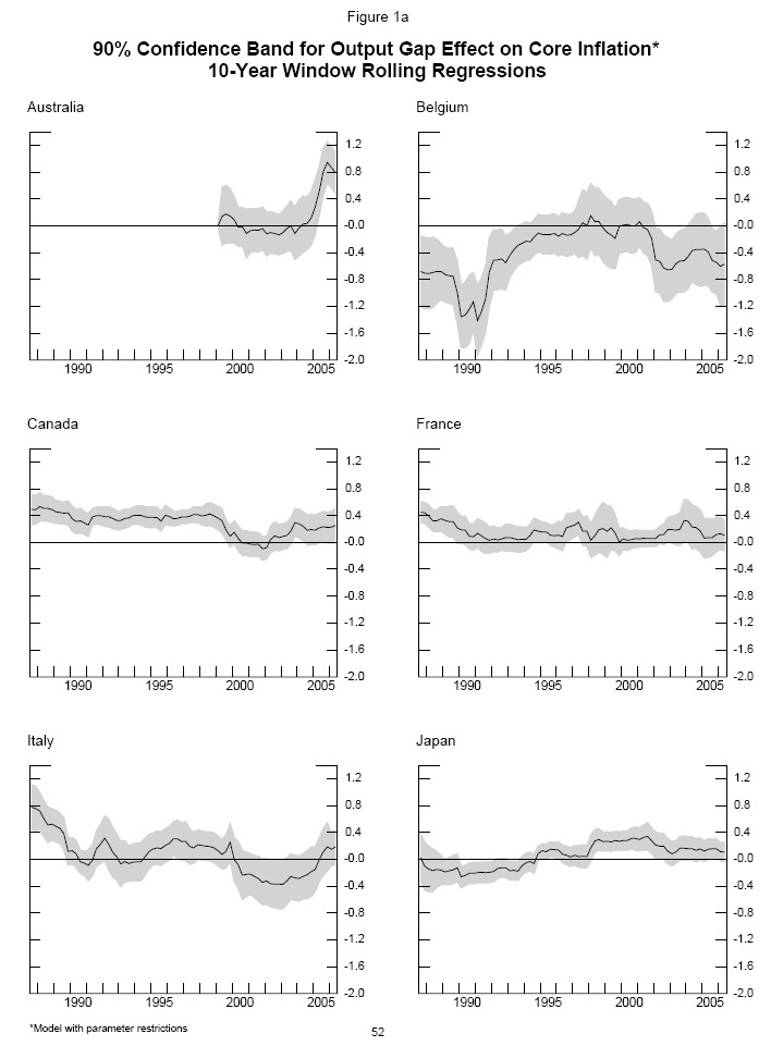
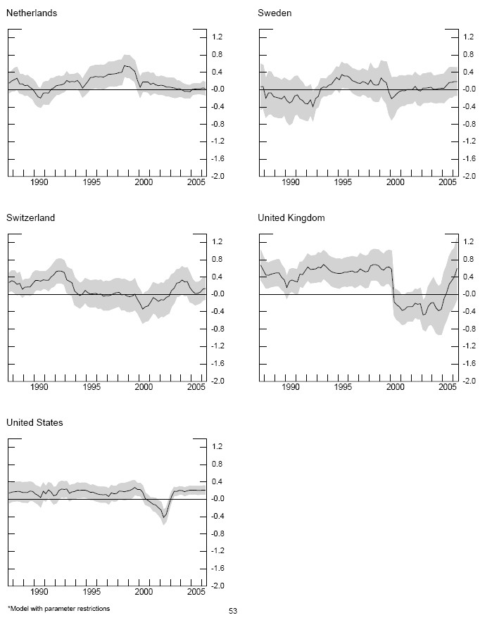
Figure 1b: 90% Confidence Band for Import-Price Effect on Core Inflation* : 10-Year Window Rolling Regressions
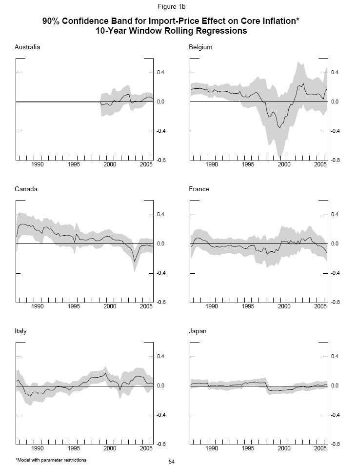

Figure 2a: Coefficient on YGAP vs. Trade Openness
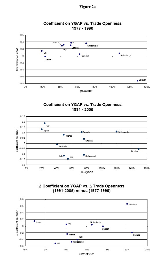
Figure 2b: Coefficient on Import Price vs. Imports/GDP
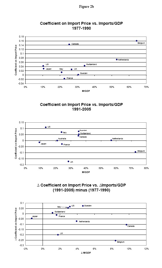
Figure 3: Rolling Correlations between Quarterly Growth Rates of Real GDP and Real Total Domestic Demand : (10-Year Window)
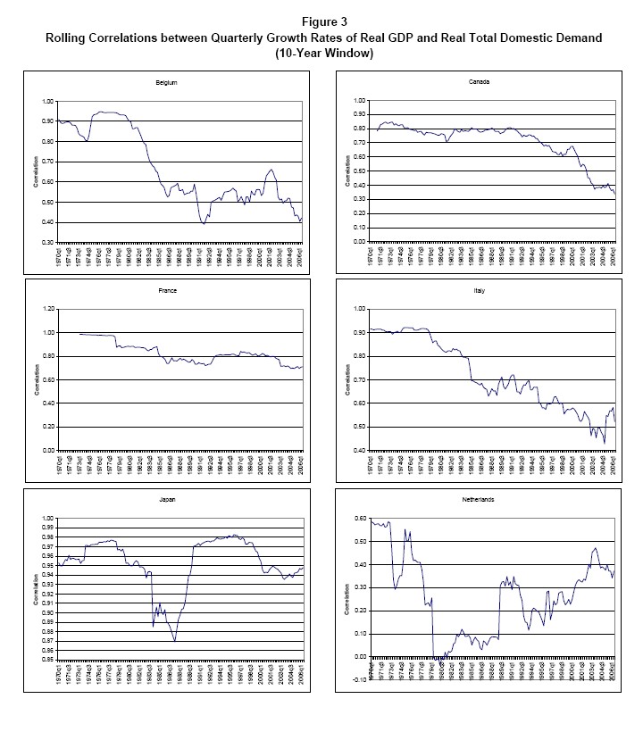
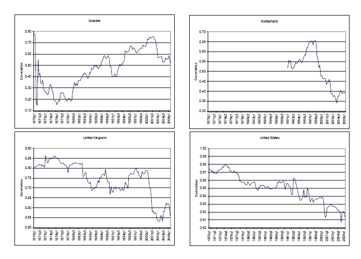
Figure 4: Absolute Value of Net Exports/GDP: 10-year Moving Average
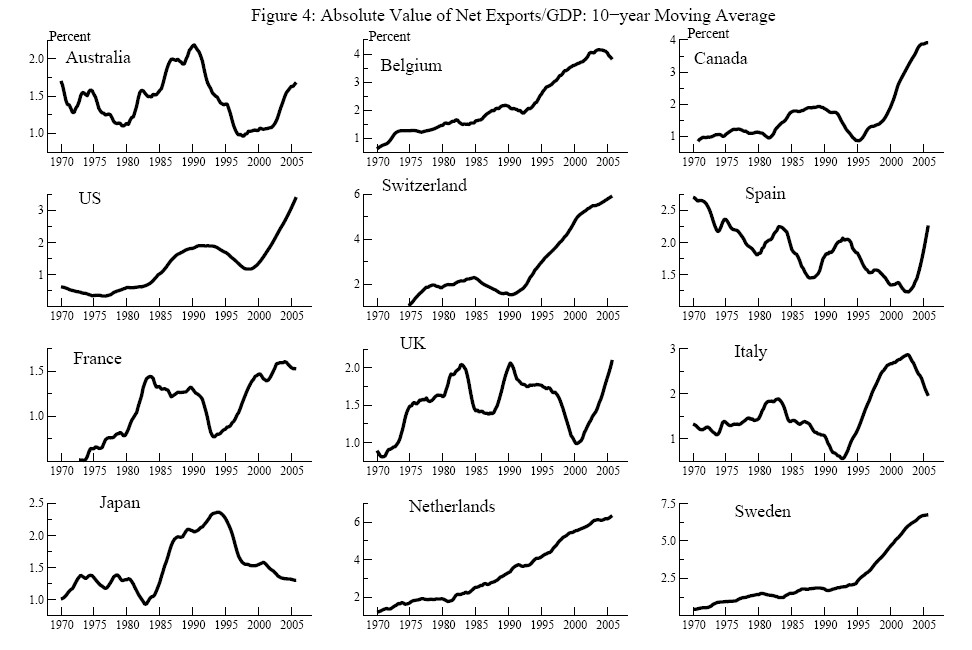
Figure 5: Rolling Covariances between Contributions of Total Domestic Demand and Net Exports to GDP : 10-Year Window)
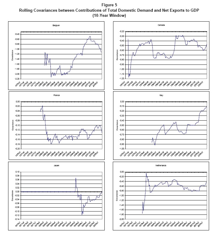
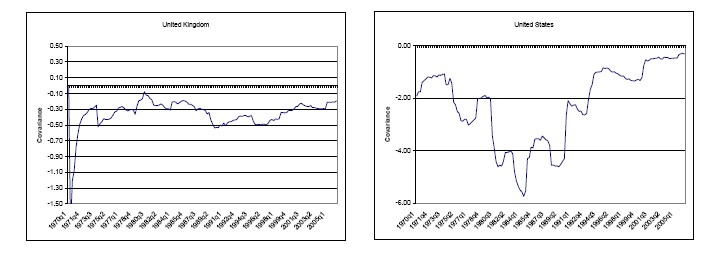
Table A1: Individual Country Tax Dummies*
(Dummies for changes in tax policies)
| Country | Tax policy change |
|---|---|
| Australia | 2000:3 |
| Austria | 1999:1 |
| Canada | 1991:1, 1994:1, 1994:2 |
| Japan | 1989:2, 1997:2 |
| Netherlands | 1991:1 |
| Sweden | 1991:1, 1992:2, 1993:1 |
| United Kingdom | 1979:3 |
* All dummies set equal to one in the appropriate quarter
Table A2: Headline Inflation*
| Australia**: Unrestricted: 77-05* | Australia**: Restricted: 77-05 | Australia**: Restricted: 77-90 | Australia**: Restricted: 91-05 | Belgium: Unrestricted: 77-05 | Belgium: Restricted: 77-05 | Belgium: Restricted: 77-90 | Belgium: Restricted: 91-05 | Canada: Unrestricted: 77-05 | Canada: Restricted: 77-05 | Canada: Restricted: 77-90 | Canada: Restricted: 91-05 | France: Unrestricted: 77-05 | France: Restricted: 77-05 | France: Restricted: 77-90 | France: Restricted: 91-05 | Italy: Unrestricted: 77-05 | Italy: Restricted: 77-05 | Italy: Restricted: 77-90 | Italy: Restricted: 91-05 | Japan: Unrestricted: 77-05 | Japan: Restricted: 77-05 | Japan: Restricted: 77-90 | Japan: Restricted: 91-05 | Netherlands: Unrestricted: 77-05 | Netherlands: Restricted: 77-05 | Netherlands: Restricted: 77-90 | Netherlands: Restricted: 91-05 | Sweden: Unrestricted: 77-05 | Sweden: Restricted: 77-05 | Sweden: Restricted: 77-90 | Sweden: Restricted: 91-05 | Switzerland: Unrestricted: 77-05 | Switzerland: Restricted: 77-05 | Switzerland: Restricted: 77-90 | Switzerland: Restricted: 91-05 | UK: Unrestricted: 77-05 | UK: Restricted: 77-05 | UK: Restricted: 77-90 | UK: Restricted: 91-05 | US†: Unrestricted: 77-05 | US†: Restricted: 77-05 | US†: Restricted: 77-90 | US†: Restricted: 91-05 | |
|---|---|---|---|---|---|---|---|---|---|---|---|---|---|---|---|---|---|---|---|---|---|---|---|---|---|---|---|---|---|---|---|---|---|---|---|---|---|---|---|---|---|---|---|---|
| Lagged inflation, sum: | 0.938 | - | - | 0.966 | 0.889 | 0.856 | 0.498 | 0.830 | 0.940 | 0.938 | 0.940 | 0.761 | 0.999 | 1.007 | 1.067 | 1.106 | 1.018 | 0.992 | 0.964 | 0.913 | 0.898 | 0.850 | 0.725 | 0.620 | 0.940 | 0.899 | 0.800 | 0.884 | 0.928 | 0.918 | 0.321 | 0.851 | 0.962 | 0.969 | 0.769 | 1.225 | 0.904 | 0.888 | 0.777 | 0.445 | 0.968 | 0.952 | 0.772 | 0.722 |
| Lagged inflation, sum: SE | 0.254 | - | - | 0.213 | 0.047 | 0.082 | 0.094 | 0.224 | 0.030 | 0.076 | 0.172 | 0.137 | 0.019 | 0.072 | 0.103 | 0.157 | 0.024 | 0.106 | 0.162 | 0.163 | 0.042 | 0.065 | 0.094 | 0.139 | 0.072 | 0.098 | 0.175 | 0.247 | 0.043 | 0.092 | 0.202 | 0.120 | 0.052 | 0.082 | 0.101 | 0.164 | 0.046 | 0.108 | 0.155 | 0.196 | 0.031 | 0.064 | 0.113 | 0.113 |
| Domestic Output Gap: | -0.1436 | - | - | -0.031 | -0.166 | -0.219 | -0.743 | -0.114 | 0.224 | 0.247 | 0.325 | 0.013 | 0.210 | 0.262 | 0.374 | 0.083 | 0.097 | 0.212 | 0.357 | -0.060 | 0.001 | 0.015 | -0.031 | 0.168 | 0.084 | 0.071 | 0.046 | 0.088 | 0.133 | 0.170 | 0.026 | 0.024 | 0.213 | 0.297 | 0.531 | -0.146 | 0.216 | 0.202 | 0.303 | -0.097 | 0.129 | 0.155 | 0.143 | 0.130 |
| Domestic Output Gap: SE | 0.134 | - | - | 0.118 | 0.095 | 0.092 | 0.139 | 0.128 | 0.046 | 0.045 | 0.072 | 0.081 | 0.051 | 0.052 | 0.085 | 0.069 | 0.076 | 0.077 | 0.131 | 0.092 | 0.040 | 0.040 | 0.060 | 0.071 | 0.044 | 0.042 | 0.080 | 0.061 | 0.070 | 0.073 | 0.238 | 0.107 | 0.084 | 0.081 | 0.092 | 0.142 | 0.087 | 0.084 | 0.129 | 0.127 | 0.043 | 0.042 | 0.085 | 0.055 |
| Import price, sum***: | -0.017 | - | - | 0.343 | 0.025 | 0.034 | 0.116 | -0.051 | 0.111 | 0.127 | 0.171 | 0.052 | -0.022 | -0.042 | 0.016 | -0.026 | 0.025 | 0.028 | 0.032 | 0.047 | 0.009 | 0.010 | 0.003 | -0.021 | 0.038 | 0.034 | 0.052 | 0.038 | 0.051 | 0.059 | -0.015 | 0.045 | 0.044 | 0.064 | 0.015 | 0.029 | -0.031 | -0.038 | -0.039 | -0.129 | 0.022 | 0.032 | 0.060 | 0.081 |
| Import price, sum***: SE | 0.042 | - | - | 0.114 | 0.026 | 0.025 | 0.026 | 0.065 | 0.026 | 0.029 | 0.060 | 0.033 | 0.035 | 0.035 | 0.065 | 0.046 | 0.025 | 0.027 | 0.066 | 0.023 | 0.014 | 0.014 | 0.017 | 0.023 | 0.033 | 0.030 | 0.050 | 0.060 | 0.040 | 0.043 | 0.068 | 0.056 | 0.029 | 0.031 | 0.041 | 0.048 | 0.047 | 0.050 | 0.085 | 0.074 | 0.025 | 0.028 | 0.041 | 0.042 |
| Food price, sum***: | 0.586 | - | - | 0.456 | 0.054 | 0.074 | 0.216 | 0.075 | -0.016 | -0.023 | -0.106 | 0.267 | 0.048 | 0.105 | -0.114 | 0.213 | 0.290 | 0.248 | 0.334 | 0.187 | 0.083 | 0.105 | 0.031 | 0.222 | 0.106 | 0.143 | 0.089 | 0.098 | 0.071 | 0.098 | 0.506 | 0.133 | 0.089 | 0.142 | 0.051 | 0.376 | 0.365 | 0.395 | 0.745 | 0.148 | 0.059 | 0.101 | 0.002 | 0.117 |
| Food price, sum***: SE | 0.309 | - | - | 0.218 | 0.047 | 0.051 | 0.058 | 0.100 | 0.043 | 0.044 | 0.071 | 0.088 | 0.049 | 0.056 | 0.125 | 0.059 | 0.089 | 0.096 | 0.228 | 0.082 | 0.056 | 0.052 | 0.096 | 0.062 | 0.061 | 0.056 | 0.126 | 0.081 | 0.065 | 0.071 | 0.183 | 0.093 | 0.039 | 0.043 | 0.057 | 0.095 | 0.153 | 0.141 | 0.212 | 0.169 | 0.046 | 0.044 | 0.087 | 0.056 |
| Energy price, sum***: | 0.065 | - | - | 0.005 | 0.057 | 0.079 | 0.128 | 0.111 | 0.033 | 0.034 | 0.044 | 0.029 | 0.003 | 0.000 | -0.037 | 0.019 | -0.0229 | 0.003 | 0.044 | 0.005 | 0.020 | 0.037 | 0.064 | 0.070 | 0.012 | 0.018 | 0.053 | 0.014 | 0.047 | 0.081 | 0.223 | 0.029 | 0.003 | 0.008 | 0.034 | 0.017 | 0.077 | 0.100 | 0.285 | 0.137 | 0.021 | 0.030 | 0.089 | 0.019 |
| Energy price, sum***: SE | 0.079 | - | - | 0.058 | 0.017 | 0.014 | 0.015 | 0.040 | 0.017 | 0.017 | 0.035 | 0.026 | 0.015 | 0.016 | 0.030 | 0.027 | 0.024 | 0.026 | 0.057 | 0.024 | 0.017 | 0.017 | 0.025 | 0.045 | 0.019 | 0.020 | 0.047 | 0.029 | 0.028 | 0.029 | 0.054 | 0.040 | 0.011 | 0.011 | 0.013 | 0.022 | 0.052 | 0.055 | 0.101 | 0.073 | 0.009 | 0.009 | 0.020 | 0.015 |
| Adj R2: | 0.696 | - | - | 0.685 | 0.884 | 0.882 | 0.945 | 0.591 | 0.941 | 0.935 | 0.914 | 0.862 | 0.976 | 0.969 | 0.963 | 0.731 | 0.958 | 0.949 | 0.913 | 0.853 | 0.914 | 0.908 | 0.916 | 0.858 | 0.809 | 0.810 | 0.849 | 0.576 | 0.897 | 0.876 | 0.779 | 0.842 | 0.884 | 0.863 | 0.914 | 0.788 | 0.869 | 0.845 | 0.859 | 0.266 | 0.957 | 0.953 | 0.954 | 0.842 |
| Adj R2: SER | 1.227 | - | - | 1.248 | 0.837 | 0.842 | 0.645 | 0.826 | 0.823 | 0.864 | 0.887 | 0.744 | 0.611 | 0.688 | 0.787 | 0.502 | 1.065 | 1.177 | 1.537 | 0.551 | 0.694 | 0.716 | 0.701 | 0.609 | 0.836 | 0.834 | 0.985 | 0.696 | 1.385 | 1.524 | 1.606 | 1.092 | 0.750 | 0.816 | 0.702 | 0.725 | 1.574 | 1.715 | 1.868 | 1.018 | 0.535 | 0.556 | 0.621 | 0.400 |
| Normality | 0.013 | - | - | 0.795 | 0.828 | 0.125 | 0.605 | 0.012 | 0.105 | 0.448 | 0.511 | 0.571 | 0.434 | 0.372 | 0.744 | 0.202 | 0.000 | 0.000 | 0.119 | 0.624 | 0.577 | 0.916 | 0.930 | 0.467 | 0.765 | 0.180 | 0.307 | 0.005 | 0.000 | 0.000 | 0.016 | 0.034 | 0.009 | 0.038 | 0.267 | 0.033 | 0.003 | 0.017 | 0.361 | 0.091 | 0.070 | 0.004 | 0.067 | 0.029 |
| Serial Independence | 0.008 | - | - | 0.001 | 0.258 | 0.026 | 0.114 | 0.746 | 0.284 | 0.296 | 0.953 | 0.741 | 0.463 | 0.234 | 0.204 | 0.461 | 0.043 | 0.575 | 0.900 | 0.399 | 0.694 | 0.294 | 0.328 | 0.835 | 0.003 | 0.630 | 0.187 | 0.977 | 0.554 | 0.409 | 0.824 | 0.154 | 0.720 | 0.018 | 0.827 | 0.498 | 0.386 | 0.085 | 0.300 | 0.300 | 0.424 | 0.423 | 0.337 | 0.437 |
| ARCH 1-4 | 0.761 | - | - | 0.063 | 0.042 | 0.039 | 0.887 | 0.396 | 0.413 | 0.930 | 0.642 | 0.705 | 0.641 | 0.935 | 0.677 | 0.403 | 0.074 | 0.157 | 0.973 | 0.755 | 0.869 | 0.930 | 0.666 | 0.930 | 0.965 | 0.943 | 0.867 | 0.829 | 0.707 | 0.378 | 0.921 | 0.900 | 0.836 | 0.951 | 0.730 | 0.967 | 0.985 | 0.788 | 0.838 | 0.446 | 0.954 | 0.962 | 0.946 | 0.786 |
* Inflation is measured as the annualized quarterly percent change in the seasonally adjusted headline CPI; equation includes constant and tax dummies
**Australian energy price data starts in 1991.
*** Annualized quarterly percent changes, difference from lagged core CPI inflation
† Inflation based on BLS current-methods seasonally adjusted Headline CPI
Normality: Jarque-Bera test
Serial Independence: Test of the hypothesis that all the coefficients in an AR(4) for the residuals are equal to zero
ARCH 1-4: Test of conditional homoskedasticity
Footnotes
* The views in this paper are solely the responsibility of the authors and should not be interpreted as reflecting the views of the Board of Governors of the Federal Reserve System or of any other person associated with the Federal Reserve System. We thank Steve Cecchetti, Joseph Gagnon, Peter Hooper, Michael Leahy, Sylvain Leduc, Ellen Meade, John Roberts, Torsten Slok, and Mark Wynne, as well as participants in workshops at American University and the Federal Reserve Board for useful comments. Sean Fahle, Stephen Gardner, and Jonas Robison provided excellent research assistance. Return to text
1. See also Fisher and Cox (2007). Charles Bean, Executive Director, Chief Economist, and member of the Monetary Policy Committee of the Bank of England, also attributes significant changes in inflation behavior to globalization. (Bean, 2006) Return to text
2. See, among others, Roberts (2006), Kohn (2007), Kroszner (2007), and Mishkin (2007). Cecchetti, Hooper, Kasman, Schoenholtz, and Watson (2007), in contrast, downplay the role of expectations in the inflation behavior of recent decades. Return to text
3. See, also, Wynne and Kersting's (2007) extensive discussion of openness, endogenous monetary policy, and inflation. Return to text
4. There is no consensus on exactly how to measure the effect on industrial-country inflation of the integration of China and other low-wage economies into the world economy. Most studies suggest that this process has lowered inflation in the United States and other industrial economies by a non-negligible, but reasonably modest, extent. However, the depressive effect of China and other low-wage countries on prices of manufactures may have been offset, to an uncertain extent, by these countries' role in boosting demand and prices of primary commodities. See Hooper, Spencer, and Slok (2007), Kamin, Marazzi, and Schindler (2006), Kohn (2006), Pain, Koske, and Sollie (2006), and Yellen (2006), among others. Return to text
5. For example, assessing the ``China effect'' typically involves gauging the effects of trade with developing countries on the evolution of import prices, whereas assessing the effect of globalization more generally on the inflation process typically involves tests of the structural stability of inflation equations for industrial economies. Return to text
6. Equation (1) represents a conventional Phillips curve model, and the research described in this paper stays within this framework throughout. There have also been some analyses of open-economy influences on inflation using a ``New Keynesian'' Phillips curve framework, including Clarida, Gali, and Gertler (2002), Andres, Ortega, and Valles (2003), and Monacelli (2003). Return to text
7. Of course, consumer prices are composed of both goods and services whereas imports are primarily goods. As a result, changes in import prices may deviate on average from consumer price inflation, which will be reflected in the constant in empirical work. Return to text
8. This premise contradicts Rogoff's (2003) argument that globalization, by causing prices to be more flexible, has led inflation to become more sensitive to domestic resource utilization. That implies a steeper Phillips curve than in the past, a prediction that, as will be discussed below, is contradicted by most empirical studies. Return to text
9. Gust and Marquez (2002) document that productivity growth in many industrialized countries stayed flat or declined in the 1990s. Return to text
10. We calculate the foreign output gap for the United States as a time-varying weighted average of the output gaps of a fixed group of 35 trading partners, with the weights based on annual U.S. bilateral imports from and exports to those countries along with measures of competition in third-party markets; we calculate foreign output gaps for the remaining 13 countries in the sample analogously using those countries' weights. By contrast, the BIS estimates of the foreign output gap involve only a country's top 10 trading partners for a given year, and use only bilateral measures of trade and other transactions for the weights; the set of trading partners may change from year to year as the composition of the top 10 changes. Return to text
11. The test consists of regressing residuals on their lagged values and then testing whether the coefficients on those lags are jointly equal to zero. Return to text
12. This specification is broadly similar to that described in Stockton (1985), except that our specification incorporates changes in relative import prices as well. Return to text
13. In the unrestricted version of equation (7), for the interaction term, each lag of the relative import price term is multiplied by the same lag of the import share; for the restricted version, the moving average of relative prices is multiplied by the contemporaneous import share. Return to text
14. Using a much less structural approach, Ciccarelli and Mojon (2006) identify common factors in inflation among OECD countries and find that those factors explain a large share of the variance in national inflation rates. Return to text
This version is optimized for use by screen readers. Descriptions for all mathematical expressions are provided in LaTex format. A printable pdf version is available. Return to text