Skip to: [Printable Version (PDF)] [Bibliography] [Footnotes]

FRB: Central Banking Before, During and After the Crisis Conference - Monetary Aggregates and the Central Bank's Financial Stability Mandate Screen Reader version ^♣

Monetary Aggregates and the Central Bank's Financial Stability Mandate*

Hyun Jeong Kim

Bank of Korea

Hyun Song Shin

Princeton University

Jaeho Yun

Ewha Womans University

March 15, 2012

Abstract:

Money is the balance sheet counterpart to bank lending. As such, highly procyclical components of money reflect incremental bank lending that may reverse abruptly as financial conditions deteriorate. Components of monetary aggregates that correspond to cross-border banking sector flows depend sensitively on both domestic and global financial factors and display a procyclical pattern that may be utilized in constructing a set of indicators of the vulnerability of the financial system to crises. We illustrate our arguments by drawing on the experience of Korea and by presenting an empirical analysis of cross-border banking flows into "demand pull" and " supply push" components.

1 Introduction

Monetary aggregates have a long history of association with central banks and at times have occupied a central position in the conduct of monetary policy. Some central banks, notably the European Central Bank, still place emphasis on monitoring monetary developments, but compared to the heyday of monetary analysis in the 1970s and 1980s, it would be fair to say that monetary aggregates have received far less attention at central banks.

The question we pose in this paper is whether monetary aggregates ought to be given a more central role once again, not with respect to their traditional role as a mirror on real activity and inflation, but instead as part of the financial stability mandate of the central bank. We ask, in particular, whether monetary aggregates may serve as signals of underlying financial conditions and the potential vulnerability of the financial system to a sharp reversal of permissive financial conditions.

In posing our question, we do not intend to suggest that the question is new. The role of monetary aggregates as the counterpart to credit developments have been well understood by central bankers (see, for instance, Issing (2003) and Tucker (2007)). Rather, our intention here is to lay out the insights drawn from the recent crisis more systematically and to do so from the perspective of an open economy subject to swings in cross-border capital flows where the forces outlined here can be expected to operate more acutely. Korea is an example of such an open economy, but the insights are equally useful for understanding capital flow reversals in the Eurozone.

The rationale for monetary aggregates as a signal of financial conditions starts with its status as the balance sheet counterpart to bank lending, or intermediated lending more generally. Procyclical components of money reflect incremental bank lending that may reverse abruptly when the cycle turns and financial conditions deteriorate. More generally, monetary aggregates may be expected to convey information on the degree of risk-taking in the economy giving insights on the vulnerability of the financial system to a reversal. In this way, monetary aggregates may play their part in the mission of central banks with respect to their financial stability mandate.

Our discussion draws on the Korean experience, and highlights the important role played by the "non-core" liabilities of the banking sector - non-traditional monetary aggregates that are highly procyclical and which are closely tied with cross-border banking. We build on the earlier findings of Hahm, Mishkin, Shin and Shin (2012), who examined the cyclical properties of monetary components in Korea, and on Hahm, Shin and Shin (2011) who examined cross-country evidence on the potential informational value of non-core liabilities in signaling increased vulnerability to a financial crisis.

Core liabilities are the funding that the bank draws on during normal times. What constitutes core funding will depend on the context and the economy in question, but retail deposits of the household sector would be a good instance of core liabilities. When banking sector assets are growing rapidly, the core funding available to the banking sector is likely to be insufficient to finance the rapid growth in new lending. This is because retail deposits grow in line with the aggregate wealth of the household sector. Other sources of funding must then be tapped to fund rapidly increasing bank lending, contributing to the growth in " non-core" funding aggregates. The state of the financial cycle is thus reflected in the composition of bank liabilities, in particular the relative size of non-core to core funding.

Cross-border banking flows are sensitive the interaction of global and local financial conditions - to the "supply push" and "demand pull" forces in operation. Our core empirical section presents an analysis of the liabilities of banks in Korea associated with cross-border banking, where we explore methods to decompose the growth of such aggrgates into "demand pull" and " supply push" components. We employ the tool of vector autoregressions (VAR) with sign restrictions where the identification of the VAR is achieved by defining a positive demand shock as one where the increase in the aggregate is accompanied by an increase in an appropriately defined spread variable (its price), while a positive supply shock is one where the increase in the aggregate is accompanied by a compression of the spread (fall in price). This method allows us to reconstruct the hypothetical evolution of the bank liability aggregates that can be attributed purely to supply shocks and purely to demand shocks. The resulting decomposition paints a revealing picture of the ebb and flow of "global liquidity", and its relationship to domestic financial stability.

We begin in the next section by outlining the main conceptual distinctions between our approach and the traditional approach to monetary analysis. We then discuss the role of cross-border banking in Section 3 and illustrate the forces at work by comparing the experience of Korea and the Eurozone with regard to the growth and subsequent reversal of cross-border banking flows. Our main empirical investigation on the decomposition of demand and supply shocks to monetary aggregates follows in Section 4. We conclude in Section 5 by drawing together the strands of the discussion and outline some policy lessons for central banks in connection with their financial stability mandate.

2 Monetary Aggregates and Procyclicality

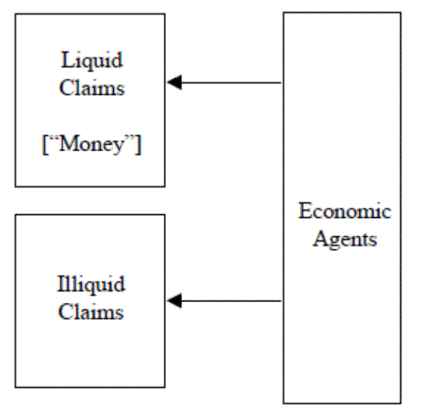
Traditionally, the importance of monetary analysis for the real economy rested on a stable money demand relationship that underpinned the link between money and macro variables. Money demand is seen as the result of a portfolio decision of economic agents choosing between liquid and illiquid claims, whether based on an inventory holding of money for transactions purposes (Baumol (1952), Tobin (1956), Miller and Orr (1966)), or as part of a more general portfolio problem between liquid and illiquid assets, but where the transactions role of money plays a role (Friedman (1956), Tobin (1958)). Figure 1 illustrates this view of money schematically.

Figure 1: Money demand as the outcome of a portfolio choice problem

For this reason, the traditional classifications of monetary aggregates focus on the transactions role of money as a medium of exchange. The criterion for the classification is based on how close to cash - how "money-like" - a particular financial claim is. Demand deposits are the archetypal money measure, since such liabilities of the banking sector can be quickly transferred from one person to another. Savings deposits are less money-like, and hence figure in broader notions of money, such as M2, but even for this they fall outside the M2 measure if the depositor faces restrictions on easy access to the funds. In this way, the traditional hierarchy of monetary aggregates goes from cash to the very liquid claims such as demand deposits going out to more illiquid claims on the banking sector such as term savings deposits. However, monetary analysis fell out of favor in the 1980s as the money demand relationship became less reliable.¹

However, unlike commodity money, monetary aggregates are the liabilities of banks and hence have an asset-side counterpart. Gurley and Shaw (1960) emphasized the distinction between "inside money" which is a liability of an economic agent and "outside money" which is not, and Brunnermeier and Sannikov (2011) have revisited the relationship between inside and outside money through the lens of bank lending decisions.

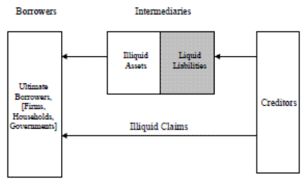
Recognizing the asset-side counterpart of money and the determinants of bank lending focuses attention on the supply of money by banks as emphasized by Brunner and Meltzer (1976). Thus, schmetically, it may be better to view the role of monetary aggregates in terms of Figure 2, rather than Figure 1.

Figure 2: Money and financial intermediation

Indeed, rather than speaking of the demand for money by savers, we could turn the relationship on its head, and speak of the supply of funding by savers. The language of funding demand and supply also has the virtue that the comparative statics of price (the interest rate) has the correct sign relative to the quantity. When the banks' demand curve for funding shifts out, the cost of funding goes up.

Most importantly, by speaking of the supply of money as the demand for funding, the shift in the language serves to focus attention on the banking sector and its balance sheet management over the cycle. When bank liabilities are increasing rapidly, households are supplying more credit indirectly through the banking sector rather than directly through some other means (e.g. through the corporate bond market). If the "as if" preferences of banks were identical to the household sector, then it would not make a difference to the projects being financed in the economy whether the funding is provided directly or indirectly. However, to the extent that the banking sector is more susceptible to procyclical behavior, lending standards vary more over the cycle than would be justified by the economic fundamentals alone. Thus, an increase in the relative size of the banking sector during a boom is likely to entail lower lending standards and greater "risk appetite" in overall lending decisions.

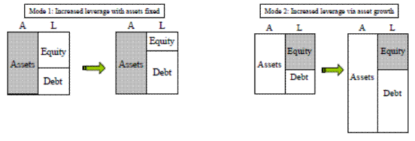
The procyclial nature of cross-border banking can be traced to the distinctive nature of banks' balance sheet management over the cycle. In textbook discussions of corporate financing decisions, the set of positive net present value (NPV) projects is often taken as being given, with the implication that the size of the balance sheet is fixed. Instead, attention falls on how those assets are financed. Leverage increases by substituting equity for debt, such as through an equity buy-back financed by a debt issue, as depicted by the left hand panel in Figure 3.

Figure 3: Two Modes of Leveraging Up

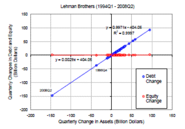
However, the left hand panel in Figure 3 turns out not to be a good description of the way that the banking sector leverage varies over the financial cycle. Instead, leverage and total assets tend to move in lock-step, as depicted in the right hand panel of Figure 3. Bank balance sheet management can be illustrated in Figure 4 that shows the scatter chart of the change debt and equity to changes in total assets of Lehman Brothers. The pattern in Figure 4 is typical of banks across countries and across business sectors, although the short-term nature of Lehman's balance sheet items illustrates the effects particularly clearly.² Figure 4 plots $\left\{ \left( \Delta A_{t},\Delta E_{t}\right) \right\}$ and $\left\{ \left( \Delta A_{t},\Delta D_{t}\right) \right\}$ where $\Delta A_{t}$ is the change in Lehman's assets at quarter , and where $\Delta E_{t}$ and $\Delta D_{t}$ are the change in equity and change in debt, respectively.

Figure 4: Scatter chart of $\left\{ \left( \Delta A_{t},\Delta D_{t}\right)$ and $\left\{ \left( \Delta A_{t},\Delta E_{t}\right) \right\}$ for quarterly changes in assets, equity and debt of Lehman Brothers, 1994Q1-2008Q2 (Source: SEC 10Q filings)

$Figure 4: Scatter chart of {(ΔAt,ΔEt)} and {(ΔAt,ΔDt)} for quarterly changes in assets, equity and debt of Lehman Brothers, 1994Q1-2008Q2 (Source: SEC 10Q filings). This is an x-y graph with Quarterly Changes in Debt and Equity (Billion Dollars) on the y-axis and Quarterly Change in Assets (Billion Dollars) on the x-axis. The range of both axes is from -200 to 150, increasing in increments in 50. There are two lines in the graph, one blue that represents Debt Change and one red that represents Equity Change. The blue line, fitted through (ΔAt, ΔDt), has a slope very close to one, with equation y=0.9971x-404.05 and R^2=0.9997. The lowest point on this line is titled 2008Q2, which has coordinates of approximately (-150, -150). Another point on this line titled 1998Q4 has coordinated of approximately (-40, -40). The red line, fitted through (ΔAt, ΔEt), has a slope that is nearly zero and essentially lies on the line y=0. The equation of the line is labeled as y=0.0029x + 404.05.$

The fitted line through $\left\{ \left( \Delta A_{t},\Delta D_{t}\right) \right\}$ has slope very close to 1, meaning that the change in lending is met dollar for dollar by a change in debt, with equity remaining "sticky". The slope of the fitted line through the points $\left\{ \left( \Delta A_{t},\Delta E_{t}\right) \right\}$ is close to zero. Both features capture the picture of bank balance sheet management given by the right hand panel in Figure 3.

Notice that the slopes of the two fitted lines add up to 1 in Figure 4. This is a consequence of the balance sheet identity: $% \Delta A_{t}=\Delta E_{t}+\Delta D_{t}$ . The sum consisting of the slope of the fitted line through $\left\{ \left( \Delta A_{t},\Delta D_{t}\right) \right\}$ and the slope of the fitted line through $\left\{ \left( \Delta A_{t},\Delta E_{t}\right) \right\}$ is given by

sum of slopes	$\displaystyle =\frac{Cov\left( \Delta A_{t},\Delta D_{t}\right) }{% Var\left( \Delta A_{t}\right) }+\frac{Cov\left( \Delta A_{t},\Delta E_{t}\right) }{Var\left( \Delta A_{t}\right) }$
	$\displaystyle =\frac{Cov\left( \Delta A_{t},\Delta D_{t}+\Delta E_{t}\right) }{Var\left( \Delta A_{t}\right) }$
	$\displaystyle =1$

Figure 5: Scatter chart of quarterly changes in assets, equity and debt of US investment banks Bear Stearns, Goldman Sachs, Merrill Lynch and Morgan Stanley (Source: SEC 10Q filings)

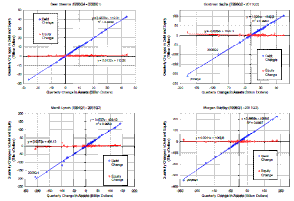
Figure 5 shows the analogous scatter plots of four other US investment banks. We see essentially the same pattern as for Lehman Brothers, where every dollar of new assets is matched by a dollar in debt, with equity remaining virtually unchanged.

The fact that banks tend to reduce debt when they shrink assets during downturns is not a surprise, as standard theories of debt overhang or adverse selection in equity issuance could explain the reluctance of banks to issue equity. However, what is notable in Figures 4 and 5 is the fact that banks do not issue equity even when assets are increasing. The fitted line through the debt issuance holds just as well when assets are increasing as it does when assets are decreasing. This feature presents challenges to an approach where the bank capital constraint binds only in downturns, or to models where the banking sector is a portfolio maximizer where leverage increases with the risk premium. Adrian, Colla and Shin (2012) explore some of the implications of these behavioral traits for modeling financial frictions in macroeconomics.

Figure 6: Total assets and risk-weighted assets of Barclays and Societe Generale (Source: Bankscope)

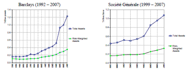
A consequence of banks' model of balance sheet management is that leverage depends sensitively on the prevailing measured risks in the financial system. During tranquil times when measured risks are low, bank lending increases rapidly to use up the slack in lending capacity as suggested by the lower perceived risks. In effect, lending expands in tranquil times so that the bank's risk constraint binds in spite of the low measured risks. Borio and Disyatat (2011) have coined the term " excess elasticity" to describe the tendency of the banking system to expand when financial constraints are relaxed. Figure 6 illustrates such excess elasticity. It plots the total assets and risk-weighted assets of two typical European global banks - Barclays and Société Générale. Even as total assets were growing rapidly up to the eve of the crisis in 2007, the risk-weighted assets of the banks were growing moderately, reflecting the low levels of measured risks, and implying low levels of equity capital on the banks' balance sheets.

The procyclical nature of banking sector balance sheet management is reflected in monetary aggregates. As intermediaries who borrow in order to lend, banks must raise funding in order to lend to their borrowers. When credit is growing faster than the pool of available domestic funding, the bank will turn to cross-border sources of funding, often in foreign currency (as in Korea), but the cross-border funding could also be in domestic currency, as in those countries in the Eurozone that underwent lending booms that fueled property booms, such as Ireland and Spain.

We may expect the cyclical properties of the bank funding aggregates to reflect distinctive patterns depending on whether the funding is a core funding category or a non-core funding category. As a foretaste of our main empirical section, Figure 7 plots various bank funding aggregates that have been filtered at business cycle frequency through a Hodrick-Prescott filter.³

Figure 7: HP-filtered monthly growth rates (log differences) of M2, non-core liabilities and FX borrowing of the Korean banking sector

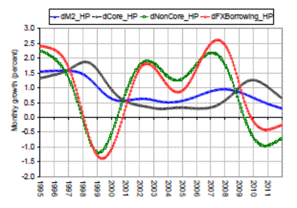
The plots show the HP-filtered monthly growth rates. The foreign exchange-denominated bank liabilities can be seen to be most procyclical, rising rapidly before the Asian financial crisis of 1997 before crashing during the crisis. Subsequently the series rises rapidly again to peak on the eve of the 2008 crisis, before falling rapidly in the aftermath of the crisis. The non-core category is a broader aggregate that encompasses foreign exchange-denominated liabilities, but also includes domestic currency bank debt securities, certificates of deposit and other wholesale funding sources (we return to the definitions in the next section). In contrast to the highly procyclical nature of the non-core liabilities, the M2 money stock is more stable, while the core liabilities category increases during crisis times reflecting flight to safety flows.

3 Money and Cross-Border Capital Flows

The link between monetary aggregates and financial stability can be traced to the role of financial intermediaries. In particular, the link can be found in the role of cross-border banking in driving fluctuations in risk premiums and financial conditions, especially in connection with the growing use of wholesale (or market-based) bank funding.

In times of rapid credit growth, the core funding sources available to banks (such as household deposits) will need to be suplemented with wholesale funding often provided through cross-border lending by global banks. Although banking sector flows are just one component of overall capital flows, it is perhaps the most procyclical component of capital flows that transmits financial conditions across borders.

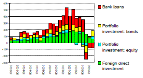
Figure 8 is a chart from the April 2010 issue of the IMF's Global Financial Stability Report showing capital flows to 41 open emerging and advanced economies disaggregated into the four main categories of capital flows. We see that aggregate FDI flows are steady and portfolio equity flows are small in net terms. However, banking sector flows display the signature procyclical pattern of surging during the boom, only to change sign abruptly and surge out with the deleveraging of the banking sector. The downward pointing bar in 2008Q4 is particularly striking.

Figure 8: Categories of capital flows to 41 open emerging and advanced economies (in billions of dollars) (Source: IMF GFSR, April 2010, p. 123)

Before embarking on our empirical investigation, we outline some lessons from Korea and explain how Korea's experience holds lessons for the recent events in the Eurozone. Although Korea and the Eurozone have outwardly very different financial systems, the perspective of the vulnerabilities generated by cross-border banking turns out to be very illuminating, although there are differences, too.

One difference is the role of the exchange rate. Korea has been vulnerable to "twin crises" in which a banking crisis and currency crisis reinforce each other. The Asian financial crisis of 1997 and the turmoil in global financial markets in the autumn of 2008 are instances of the vulnerability. Such crises are particularly damaging due to the mutually reinforcing nature of the two crises, and the rapid deterioration of economic fundamentals caused by the amplification of the crisis. For the countries in the Eurozone, the currency mismatch does not exist.

However, there are important parallels in the behavior of banking sector liabilities. Bank lending growth is mirrored on the liabilities side of the balance sheet by shifts in the composition of bank funding. In a lending boom when credit is growing very rapidly, the pool of retail deposits is not sufficient to fund the increase in bank credit. Other sources of funding are tapped to fund rapidly increasing bank lending. The state of the financial cycle is thus reflected in the composition of bank liabilities.

Figure 9: Six categories of non-core bank liabilities in Korea (right panel) and time series of the ratio of non-core to M2 in Korea (left panel) (Source: Shin and Shin (2010) and Bank of Korea)

$Figure 9: Six categories of non-core bank liabilities in Korea (right panel) and time series of the ratio of non-core to M2 in Korea (left panel) (Source: Shin and Shin (2010) and Bank of Korea). Figure 9 has two panels. The left panel is a graph titled Non-core Liabilities as Fraction of M2, with the y-axis labeled with the fraction amount (range from 0.10 to 0.55) and the x-axis labeled as the date (from Jan-91 to Jan-10). The line begins at 0.15 in Jan-91 and increases to 0.3 in Jan-98 before dropping drastically to 0.15 in Jan-99. It then steadily increases to peak at 0.50 in Jan-09 before coming down to 0.35 by Jan-10. The right panel shows the composition of non-core bank liabilities in six categories. The y-axis is labeled Trillion Won (range from 0-800) and the x-axis is labeled with dates, from Jan-91 to Jan-09. The six categories are [M2] Certificate of Deposit, [M2] Promissory Note 1, [M2] Promissory Note 2, [Lf] Repos, [Lf] Debt Securities, and [Other] FX borrowing. The total value at Jan-91 is approximately 20, and steadily increases to 180 at Jan-98. The main component is FX borrowing, which takes up over half, followed by smaller contributions from Debt Securities and Repos, and minimal contributions from the other categories. The total value then dips to 100 in Jan-01 before increasing dramatically to peak at 700 in Jan-08, before coming down to 550 in Jan-09. During this time, the presence of Debt Securities increased dramatically, such that it held the same ratio to the total as FX borrowing. Certificate of Deposits also increase its presence, ending at around 100 of the total 550 at the end of the graph.$

In Korea, rapid increases in the non-core liabilities of the banking system show up as capital inflows through increased foreign exchange-denominated liabilities of the banking system. The right hand panel of Figure 9 charts the non-core liabilities of the Korean banking sector, taken from Shin and Shin (2010) with the FX liabilities shown at the top of the chart. Note that the first peak in non-core liabilities coincides with the 1997 crisis. After a lull in the early 2000s, non-core liabilities increase rapidly in the run-up to the 2008 crisis.

The left hand panel of Figure 9 plots the non-core liabilities as a fraction of M2. We see that there has been substantial variation in non-core liabilities, ranging from around 15% of M2 to a peak of 50% in the Lehman crisis. Hahm, Shin and Shin (2011) conduct a cross-country probit analysis on the vulnerability of an economy to a financial crisis, and find that the incidence of banking sector liabilities to foreigners is consistently the most reliable signal of vulnerability to a crisis.

3.1 Parallels with the Eurozone

The role of monetary aggregates as signals of vulnerability can supply insights in understanding recent stresses in the Eurozone.

Figure 10: Growth rate of eurozone M1, M2, and M3 money stocks. Six month growth rates are shown and growth is defined as log differences (Source: ECB)

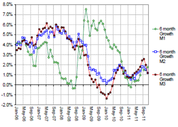
Figure 10 plots the six month growth rate of the M1, M2 and M3 money stock in the eurozone for the period from 2006. The divergent patterns of growth between M1 on the one hand and M2 and M3 on the other are quite striking. We see that in the crisis period associated with the failure of Lehman Brothers, M1 experienced rapid growth but M2 and M3 showed a marked slowing of growth. Indeed, M3 growth turns negative in late 2009 and early 2010.

To delve deeper into the reasons for the divergence of the standard monetary aggregates, we examine the movements in the individual components of the monetary aggregates. The table below presents the definition of the monetary aggregates used by the European Central Bank.

Table 1: Definition of eurozone M1, M2, and M3 stocks (Source: European Central Bank)

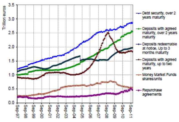
We can see that the difference between M1 and M2 consists of time deposits up to two years maturity and deposits that are redeemable at a period of notice up to three months. The divergent paths between M1 and M2 suggests that one or both of these incremental components of M2 should show a time series pattern that is quite distinctive relative to M1.

Figure 11: Components of eurozone monetary aggregates (Source: ECB)

Figure 11 plots aggregate liability items of the eurozone banking sector that correspond to the components of the various monetary aggregates in the eurozone.

The series that stands out is the one for time deposits of up to two years maturity. The series hovers around 1 trilliion euros until roughly 2005, but then begins a period of rapid growth, reaching 2.5 trillion euros on the eve of the Lehman crisis in 2008. The time series pattern displayed by this series is quite distinctively procyclical, suggesting strongly that this series is associated with the growth in cross-border bank lending within the eurozone.

In any case, it is noteworthy how different the cyclical patterns are of the varios components of the standard monetary aggregates. Since these are aggregates for the whole of the Eurozone, they do not reflect the regional shifts in deposits away from the crisis-sticken countries toward the core countries. Instead, it is likely that the divergent patterns reflect the differing identities of the claim holders - in particular, between the banking sector and non-banks.

Another perspective on the growth of eurozone cross-border banking growth can be obtained from the BIS locational banking statistics. Figure 12 plots the cross-border assets and liabilities of eurozone banks in euros. The destination of euro-denominated lending reached outside the eurozone, as eurozone banks expanded into central and eastern Europe. However, the cross-border euro-denominated liabilities series in Figure 12 is more illuminating, since it is the series that mostly closely approximates the cross-border banking liabilities aggregates that are the focus of our paper.

Figure 12: Cross-border euro-denominated claims and liabilities of eurozone banks (Source: BIS Locational Statistics, Table 5A)

Figure 13: Four quarter growth rate of cross-border euro-denominated liabilities of eurozone banks (Source: BIS Locational Banking Statistics Table 5A)

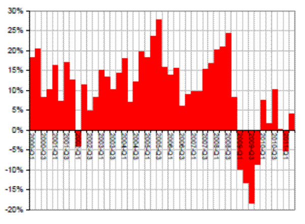
Figure 13 plots the four-quarter growth rates in cross-border euro-denominated banking sector liabilities. From 1999Q1 to 2008Q3, cross border liabilities rose almost 3.5-fold from 1.56 trillion euros to 5.4 trillion euros. This rapid spurt translates into a constant quarterly growth rate of 3.33%, which when annualized is close to 14%.

An annual growth rate of 14% sustained for such a lengthy period is unusual and is reminiscent of the growth in banking sector liabilities that accompanied the 1980s bubble in Japan. Hattori, Shin and Takahashi (2009) show that the component of banking sector liabilities that experienced most rapid growth in the bubble years of the late 1980s were time deposits, drawing a parallel with the procyclical behavior of the growth in eurozone time deposits up to two years maturity in Figure 11.

Given the highly procyclical nature of such flows, monitoring such aggregates may give us insights on the build-up of vulnerabilities in the financial system, although any formalized rule and threshold level of growth may be subject to the usual argument that behavior will change so as to nullify the initial rule - a version of Goodhart's Law. Nevertheless, monetary aggregates that are known to be highly procyclical may be informative as a warning signal on the build-up of potential vulnerabilities to the financial system.

The growth in cross-border banking liabilities reflect the growing reliance on wholesale funding by banks in Spain, Ireland and other economies experiencing booms in the residential property market on the back of strong growth in bank lending. In this respect, the Korean experience and the experience of the Eurozone have considerable overlap. The key similarity is the role played by cross-border banking sector liabilities. To the extent that such liabilities are monetary aggregates - albeit non-traditional ones in the case of Korea - monitoring carefully selected specific monetary aggregates may yield insights into the build-up of vulnerabilities to a sudden reversal of such flows.

4 Disentangling Domestic and Global Factors

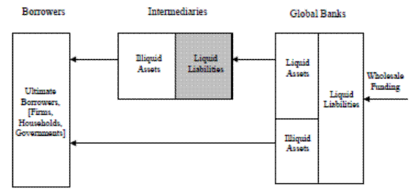
We now turn to consider the underlying economic variables that explain the growth of foreign exchange-denominated liabilities of the banking sector. To the extent that global liquidity conditions affect capital inflows through the banking sector, the answer to this question entails viewing the problem as a larger whole where global banks themselves are part of the picture, as in Figure 14. This figure develops the basic picture of monetary aggregates as arising from investor portfolio decisions in two ways. We have already noted that there is an asset side counterpart to the monetary aggregates. Figure 14 also points to the importance of understanding the creditor to the banking sector. When cross-border banking flows are involved, the creditor may itself be an intermediary - a global bank, perhaps, which borrows in order to lend. Thus, when global liquidity conditions ease due to more permissive global financial conditions, the "supply push" factor in capital inflows through the banking sector may be important as well as the "demand pull" component due to the expansion of lending by domestic banks.

Figure 14: Global banking and monetary aggregates

4.1 Demand Pull and Supply Push

In the case of cross-border banking, both "demand pull" and "supply push" forces will operate to determine total cross-border flows and financial conditions in the recipient economy. Bruno and Shin (2011) has examined a model of the determination of cross-border banking flows and the resulting impact on financial conditions. We sketch the outlines of the model here to inform our empirical study below.

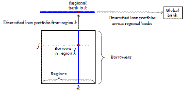
Consider the following "double-decker" version of the well-known Vasicek (2002) credit risk model that has served as the backbone to the Basel capital rules (BCBS (2005)). In the model, there is continuum of borrowers of unit mass, each of whom is assigned to a particular region, as depicted in Figure 15.

Figure 15: Global and regional banks

The square box in Figure 15 represents the population of borrowers across all regions. Regional bank holds a portfolio that is diversified against idiosyncratic shocks across borrowers in its own region, but not to regional shocks. Global banks hold a portfolio of loans to regional banks, and is diversified against regional shocks, but it faces undiversifiable global shocks.

Specifically, borrower in region defaults when the realization of the following random variable is negative.

$\displaystyle Z_{kj}\equiv -\Phi ^{-1}\left( \varepsilon \right) +\sqrt{\rho }Y_{k}+\sqrt{% 1-\rho }X_{kj}$

(1)

where

$\displaystyle Y_{k}=\sqrt{\beta }G+\sqrt{1-\beta }R_{k}$

(2)

In (1), $Y_{k}$ and $\left \{ X_{kj}\right \}$ are standard normal random variables, with the interpretation that $X_{kj}$ is the idiosyncratic risk factor for borrower in region , while $Y_{k}$ is the region-wide risk factor that affects all borrowers in region . The parameter $\rho \in \left( 0,1\right)$ gives the systematic risk in the loan portfolio. The cdf of the standard normal is denoted by $\Phi \left( .\right)$ in (1), and the unconditional probability of default of any loan is $% \varepsilon$ since

$\displaystyle \Pr \left( Z_{kj}<0\right) =\Pr \left( \sqrt{\rho }Y_{k}+\sqrt{1-\rho }% X_{kj}<\Phi ^{-1}\left( \varepsilon \right) \right) =\Phi \left( \Phi ^{-1}\left( \varepsilon \right) \right) =\varepsilon$

Suppose that regional banks follow the Value-at-Risk rule in which they keep enough equity to limit failure to probability $\alpha$ , and the global banks lend to the regional banks. The Value-at-Risk threshold $\alpha$ followed by regional banks is then the probability of default by the regional bank on its loan from the global bank. The global bank can diversify across regions by lending to a continuum of regional banks, but cannot diversify away the global risk that applies to all regions. The global risk is modeled as in (2), where the regional risk factor $% Y_{k}$ is further decomposed into a purely regional risk factor $R_{k}$ that affects lenders in region and a global risk factor that affects all private credit recipients everywhere. The random variables $G,\left\{ R_{k}\right\}$ and $\left \{ X_{kj}\right \}$ are mutually independent standard normals.

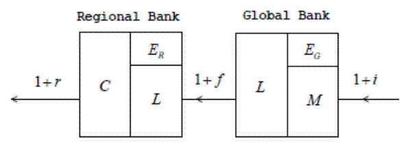
Given this three factor structure of global, purely regional and idiosyncratic risk factors, the model can be solved in closed form for the cross-banking flows (see Bruno and Shin (2011)). To introduce the closed form solutions, we introduce the notation in Figure 16. The regional banks provide private credit (denoted ) to local borrowers at the rate . This private credit is funded by cross-border liabilities (denoted by ) drawn from the global banks at the funding rate . For the global banks, the cross-border lending appears on the asset side of the balance sheet, and the funding rate is the rate earned on its assets. The global banks finance themselves by drawing on wholesale money market funds at the interest rate . The equity of the regional bank is denoted by $E_{R}$ while the equity of the global bank is denoted by $E_{G}$ . As we will see shortly, our model has an aggregation property across banks, so that $E_{R}$ and $E_{G}$ can be interpreted as the aggregate banking sector capital of the regional banks and global banks, respectively.

Figure 16: Regional and global bank balance sheets

In accordance with bank balance sheet management principles illustrated in the scatter charts we have encountered already, the exogenous variables are the equity terms $E_{R}$ and $E_{G}$ and the funding rate for the global banks, while the key endogenous variables are the total credit supply by regional banks and their demand for cross-border funding given by $L_{D}$ , which have closed form solutions

$\displaystyle C=\frac{E_{R}}{1-\frac{1+r}{1+f}\cdot \varphi }$ and $\displaystyle L_{D}=% \frac{E_{R}}{\frac{1+f}{1+r}\cdot \frac{1}{\varphi }-1}$

(3)

where $\varphi$ is the ratio of notional assets to notional liabilities of the regional bank. We can interpret $\varphi$ as the normalized leverage measure of the regional banks. In turn, the supply of cross-border funding by the global banks can be solved as

$\displaystyle L_{S}=\frac{E_{G}}{1-\frac{1+f}{1+i}\psi }$

(4)

where $\psi$ is the normalized leverage measure of the global banks.

Equilibrium cross-border lending through the banking sector can be obtained by setting $L_{D}=L_{S}$ and solving out equilibrium the funding rate . The funding rate can be solved as

$\displaystyle 1+f=\frac{1}{\mu \frac{1}{\left( 1+r\right) \varphi }+\left( 1-\mu \right) \frac{\psi }{1+i}}$

(5)

where

$\displaystyle \mu =\frac{E_{G}}{E_{G}+E_{R}}$

(6)

The closed form solutions for capital inflows into the recipient economy and its total lending to regional borrowers can be obtained as follows

$\displaystyle C=\frac{E_{G}+E_{R}}{1-\frac{1+r}{1+i}\varphi \psi }$ and $\displaystyle % L=\frac{E_{G}+E_{R}\cdot \frac{1+r}{1+i}\varphi \psi }{1-\frac{1+r}{1+i}% \varphi \psi }$

(7)

In longhand, these equilibrium solutions can be written as follows.

$\displaystyle \begin{tabular}{c} Total private \\ credit\end{tabular}% =\frac{\text{Aggregate bank capital (regional + global)}}{1-\text{ spread}% \times \!% \begin{tabular}{c} regional \\ leverage\end{tabular}% \! \times \!% \begin{tabular}{c} global \\ leverage\end{tabular}% }$

(8)

$\displaystyle \begin{tabular}{c} Total capital inflow \\ in banking sector\end{tabular}% =\frac{\text{Weighted bank capital (regional + global)}}{1-\text{ spread}% \times \!% \begin{tabular}{c} regional \\ leverage\end{tabular}% \! \times \!% \begin{tabular}{c} global \\ leverage\end{tabular}% }$

(9)

where "leverage" refers to the normalized leverage measures $\varphi$ and $\psi$ that are constained to lie between 0 and 1, and "spread" refers to the ratio of lending rate in the recipient economy to the funding rate for global banks.

We can interpret as the component of the monetary aggregate in the recipient economy that corresponds to the most procyclical element of capital flows given by cross-border bank lending by global banks. In this respect, the solution for is particular useful, since we can attribute the relative importance of the demand pull and supply push forces. From the solution, we see that the procyclical monetary aggregate component of the recipient economy is increasing in the leverage of the local and global banks and increasing in the spread between the local lending rate and wholesale funding rate of global banks. In addition, strong bank profitability both locally and globally increase cross-border lending through higher levels of bank equity capital, $E_{G}$ and $E_{R}$ .

The monetary component is likely to convey useful information on overall financial conditions, both domestically and globally. Note in particular that the solution for reflects both "demand pull" and "supply push" forces. The equilibrium expression for the funding rate will similarly reflect the demand and supply conditions.

In the simple model sketch above, the asset side and liabilities side convey the same information on credit availability. However, in practice, there are strong arguments for favoring the liabilities side measure - i.e. monetary aggregates - as information sources for financial conditions. In contrast to the asset side of a bank's balance sheet, the liabilities side components display distinctive cyclical patterns and allow the identification of components that differ according to their degree of procyclicality. For this reason, components of monetary aggregates that correspond to cross-border banking flows may be a useful part of the overall toolkit used by central banks in monitoring domestic financial conditions.

4.2 Empirical Investigation

We now turn to our empirical decomposition of monetary aggregate changes into their demand and supply-led components. We focus on two monetary aggregates in particular - the non-core liabilities of the Korean banks introduced in the previous section, and the FX-denominated sub-component of non-core liabilities.

Our decomposition relies on a vector autoregression (VAR) with sign restrictions, where the demand and supply shocks are identified through a restriction on the contemporareous impulse responses. Demand shocks are those that increase the quantity at the same time as raising some price measure or decrease both the quantity and the price. In contrast, supply shocks are those that move the quantity and price in opposite directions.

VAR with sign restrictions was used by Faust (1998) in his study of monetary shocks in the United States, and the theory was developed more fully by Uhlig (2005). A two variable VAR with sign restrictions for demand and supply shocks for monetary aggregates was used by Chadha, Corrado and Sun (2010) to examine the evolution of monetary aggregates in the United States and the Eurozone. We follow the methodolgy of Chadha et al. closely here.

Our VAR models include two variables - one representing a monetary aggregate (domestic non-core liabilities or FX liabilities) and the other representing a spread variable indicating the tightness of financial conditions. One price variable we use is the covered interest parity (CIP) deviation defined as

CIP deviation $\displaystyle =$ 3-month CD rate $\displaystyle -$ 3-month dollar LIBOR rate $\displaystyle -$ 3-month swap rate

(10)

We can interpret the CIP spread as the carry trade margin earned by a currency trader who borrows US dollars in the three month LIBOR market, then swaps the US dollars into Korean Won in the swap market through a three month swap contract, and then invests the proceeds in certificates of deposit (CDs) in Korea. When the CIP spread is high, the return to the carry trade (long position in Korean Won short in dollars) yields a high return.⁴ Thus, the CIP spread can be interpreted as the cost of funding obtained from the global capital markets for investment in Korea. When the Korean financial market is distressed, we would expect the CIP spread to be high.

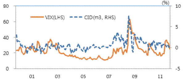
Figure 17: VIX index and the 3 month Covered Interest Parity deviation (CID)

Figure 17 plots the CIP deviation series (CID) in the Korean FX market together with the VIX implied volatility on the S&P index options, which is widely used as a measure of risk appetite in global financial markets. We see that the CIP deviation is closely aligned with VIX in the global market.

However, there are also some notable differences. Although the VIX became very compressed in the middle years of the last decade, we see that the CIP spread did not follow the VIX down. One conjecture is that the CIP was kept up by the demand for wholesale funding as carry trade inflows accelerated in the mid-2000s. This conjecture seems promising in part due to the "hump" seen in the CIP in 2007, before the financial crisis began in earnest in 2008. We return to this observation below, once we have decomposed the FX liability aggregate of Korean banks into supply and demand-led components.

Our Bayesian VAR uses monthly money stock and spread variables using data for Korean monetary aggregates covering the period from January 2000 to December 2011. Based on the unit-root tests, we take the log-difference for monetary aggregates, and use spread variables in levels.

We will focus particular attention on the non-core liabilities of the Korean banking sector, especially the sub-component that consists of the foreign currency liabilities of the banking sector.

The non-core liabilities were introduced in the previous section. It is defined as the sum of (i) bank FX liabilities (ii) bank debt securities, (iii) promissory notes (iv) repos and (v) certificates of deposit. Of the non-core liabilities total, we examine the bank FX liabilities as a separate component from the others, and examine the domestic non-core liabilities in a separate VAR.

When we run the VAR for the FX liability component by itself, we convert the sum into US dollars to adjust for possible confounding effects that arise from sharp exchange rate changes during crises. Domestic non-core liabilities comprises the last four components (ii)-(v) in the list of non-core liabilities, and the series is denominated in Korean Won.

The price variables used are as follows. For the VAR for FX liabilities of the banking sector, we use the covered interest parity CIP variable defined above. Higher CIP spreads indicate a worse FX borrowing environment for Korean banks.

For the VAR using domestic non-core liabilities, we use the corporate bond credit spread, defined as the difference between the three year yield on the corporate bond issued by AA- rated Korean firms and the government bond yield of the same maturity.

4.3 Methodology

We now outline how we have run the sign-restriction VAR model and how we have used the identified shocks to reconstruct the historical contributions of money supply and demand shocks to each endogenous variable. For the methodology, we broadly follow Chadha et al. (2010). Consider the following reduced-form VAR of order p:

$\displaystyle Y_{t}=B\left( L\right) Y_{t-1}+u_{t}$

(11)

where $Y_{t}=\left( R_{t},\Delta m_{t}\right) ^{\prime }$ is the vector of price and quantity pairs. $R_{t}$ indicates a risk spread variable which may be a CIP (covered interest rate parity) deviation or credit spread, depending on the model considered, and $\Delta m_{t}$ indicate the log-difference of monetary aggregate variables like domestic noncore liability or FX liabilities of banking sector. The lags of VAR models are chosen based on the majority rule using several lag-length criteria like AIC, SC and HQ criteria.

The above reduced-form VAR can be tranformed into the following moving average representation:

$\displaystyle Y_{t}=(I-B\left( L\right) L)^{-1}u_{t}$

(12)

Now, by imposing sign restrictions, we identify money-supply and demand shocks orthogonal to each other. We denote a $2\times 1$ structural shock vector by $\varepsilon _{t}$ where $E(\varepsilon _{t}\varepsilon _{t}^{\prime })=I_{2}$ , where $I_{2}$ is the $2\times 2$ identity matrix. We assume that the following sign restrictions hold for contemporaneous impulse responses of the endogenous variables to the structural shocks. Our restrictions are relatively weak compared to other sign-restriction VAR studies (such as Uhlig (2005) and Chadha et al. (2010)) where sign restrictions hold for a few periods after a shock occurs.

	$R_{t}$	$\Delta m_{t}$
Supply shock		-
Demand shock

For identification, our task is to find a $2\times 2$ matrix A such that $% u_{t}=A\varepsilon _{t}$ , or equivalently $\Sigma \equiv E\left( u_{t}u_{t}^{\prime }\right) =AE(\varepsilon _{t}\varepsilon _{t}^{\prime })A^{\prime }$ . What follows is a vector autoregressive moving average (VARMA) representation with orthonormal structural shocks:

$\displaystyle Y_{t}=(I-B\left( L\right) L)^{-1}A\varepsilon _{t}.$

(13)

where, by expanding $(I-B\left( L\right) L)^{-1}A$ , one can recover impulse respone functions.

In order to obtain valid candidates for matrix , we implement a Cholesky factorization of $\Sigma$ , resulting in a lower triangular matrix such that $\Sigma =TT^{\prime }$ . This indicates that $u_{t}=T\eta _{t}$ with $% E\left( \eta _{t}\eta _{t}^{\prime }\right) =I$ . The following VAR representation is the same as the one from the usual recursive VAR :

$\displaystyle Y_{t}=(I-B\left( L\right) L)^{-1}T\eta _{t},$

(14)

However, although $\eta _{t}$ is a vector consisting of orthogonal shocks, may not be a valid candidate for matrix because the Cholesky factorization does not guarantee that the sign restrictions are satisfied. In order to find a valid candidate for matrix , we introduce an orthonormal rotation matrix $2\times 2$ matrix $Q\left( \theta \right)$ such that $Q\left( \theta \right) ^{\prime }Q\left( \theta \right) =Q\left( \theta \right) Q\left( \theta \right) ^{\prime }=I.$

Concretely, we adopt the following Givens matrix for the rotation matrix $% Q\left( \theta \right)$ :

$\displaystyle Q\left( \theta \right) =\left[ \begin{array}{cc} \cos \theta & -\sin \theta \\ \sin \theta & \cos \theta \end{array}% \right] ,$

(15)

where $0<\theta <\pi .$ Using the $Q\left( \theta \right)$ matrix, we obtain the following VARMA representation :

$\displaystyle Y_{t}=(I-B\left( L\right) L)^{-1}TQ\left( \theta \right) ^{\prime }Q\left( \theta \right) \eta _{t},$

(16)

where, for suitably chosen $\theta$ satisfying the sign restrictions, we can define $A\equiv TQ\left( \theta \right) ^{\prime }$ and $\varepsilon _{t}\equiv Q\left( \theta \right) \eta _{t}$ such that $u_{t}=TQ\left( \theta \right) ^{\prime }Q\left( \theta \right) \eta _{t}$ .

Like Chadha et al. (2010) and Peersman (2005), we adopt a Bayesian approach for estimation and inference of the sign-restriction VAR model. We follow Uhlig (2005) in using a weak prior from which a posterior distribution depends only on the maximum likelihood estimator of the VAR model. See Uhlig (2005) for the functional forms of both prior and posterior distributions. Both prior and posterior distributions belong to the Normal-Wishart family, so we can easily follow a usual Gibbs-sampling procedure.

To draw the candidate shocks satisfying our sign restrictions from the posterior distribution, we take a joint draw from the posterior for the Normal-Wishart posterior for the VAR parameters as well as a uniform distributions for the rotation matrix parameter $\theta .$ We keep those shocks that satisfy our sign restrictions and discard the ones that fail. This procedure is iterated until 200 draws satisfying the sign restrictions are collected. Based on the collected 200 draws, we use the median values as paremeter estimates, together with the 84th and 16th percentile error bands which correspond to one-standard deviation confidence interval. We can then recover the historical contributions of each structural shocks by using both impulse response functions and identified structural shocks.

4.4 Empirical Results

4.4.1 FX Liabilities and CIP Spread

Figure 18 plots the impulse responses of the demand and supply shocks to the CIP spread and FX liabilities variables. As designed, the supply shocks induce changes of opposite signs into price and quantity, while the demand shocks induce changes of the same sign in price and quantity.

Figure 18: Impulse responses of CIP and changes in foreign currency-denominated liabilities of the Korean banks to a standard deviation of demand and supply shocks. (Note: The solid line is median response and the dotted lines are 14% and 86% percentile error bands. Sign restrictions and Bayesian methods to derive the impulse responses are explained in the text.

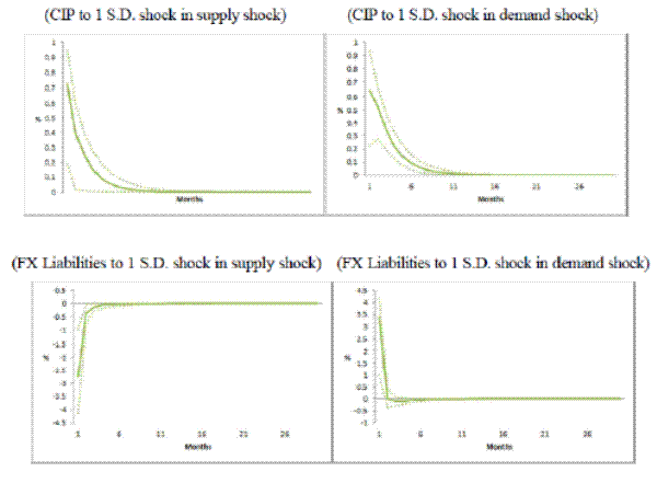
Figure 19: Historical decomposition of monthly growth in FX liabilities of the Korean banking sector (top panel) and the covered interest parity (CIP) spread (bottom panel). The charts show the 12-month moving averages of identified demand and supply shocks on FX liabilities and CIP spread from contemporaneous impulse response in the VAR. Data are from the Bank of Korea.

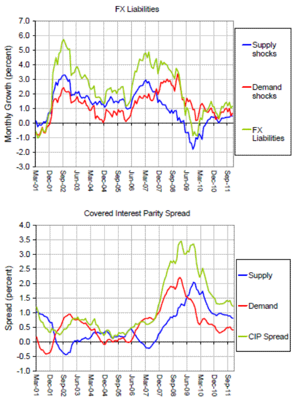
Figure 19 presents the decomposition of the FX liabilities of Korean banks (top panel) and the CIP spread (bottom panel) into the demand and supply-induced components. There are several features of note in these charts.

In terms of the quantities, we see that the initial acceleration of the FX liabilities of Korean banks was supply-led, but as the banking sector boom reached its mature stage in 2007 the demand-led growth takes over until the onset of the Lehman crisis in 2008. The supply-led component begins its decline much earlier than the demand-led component.

One possible interpretation of this shift from supply-led to demand-led growth is that the internal amplifying dynamics of the boom in the Korean banking sector gained sufficient momentum in the late stages of the boom to overcome the decline in supply-led capital inflows. Note, in particular, that the supply-led capital inflows peaks in March of 2007 and begins to decline. This pattern is consistent with the early stages of the subprime crisis in the United States and Europe where global banks will already have been under funding pressure in 2007. The supply conditions continue to deteriorate with the outbreak of the Lehman crisis, and continues to fall until reaching a trough in late 2009. Meanwhile, the demand-led component of FX liabilities reaches a peak around the Lehman crisis and declines sharply as the economy slows.

The pattern observed in the CIP spread in the bottom panel of Figure 19 paints a picture that is consistent with the quantities. We see that the CIP spread has distinct demand-led and supply-led stages. From mid-2006, we see that the demand-led CIP spread component increases, perhaps reflecting the greater demand for domestic Korean assets for carry trade positions, but this initially demand-led increase gives way to the increase in CIP due to the supply-led component from 2007 onwards, reflecting the tightening global financial conditions with the subprime crisis.

We noted above when comparing the CIP spread with the VIX index that the CIP spread remained elevated in the mid-2000s even as the VIX index plumbed new lows. The discrepancy between the VIX and the CIP spread may possibly be attributed to the demand-led increase in the CIP spread reflecting the greater demand for Korean financial assets to feed the growing carry trade positions.

Figure 20: Short-term FX liabilities of domestic Korean banks and foreign bank branches in Korea (Source: Bank of Korea)

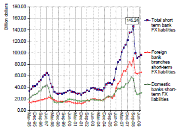
Although we have dealt with the demand and supply-led components purely with the sign restriction, the exact dividing line between demand and supply needs to be understood in the institutional context.

It is important to recognize that the FX liabilities of foreign bank branches in Korea is classified together with domestic Korean banks as being part of the banking sector FX liabilities. Such a classification is consistent with the residence principle of the balance of payments. However, to the extent that the foreign bank branches are the outposts of the global banking organizations in Korea, we may also interpret their lending as being part of the global supply of wholesale funds. The magnitudes attributable to the foreign bank branches are also very large, as seen in Figure 20). Even in absolute quantities, the FX liabilities of foreign bank branches are of comparable magnitude to the domestic Korean banks. Thus, when reading the VAR decompositions, we should bear in mind that even the demand-led component reflects in part the availability of funding in the global wholesale funding market through the operation of foreign bank branches.

4.4.2 Domestic Non-Core Liabilities

We now turn to the domestic component of non-core liabilities that strip out the FX liabilities of the banking sector. The domestic non-core liabilities are denominated in Korean Won. The price variable used is the three-year corporate bond spread, given by the difference between the yield on a three-year AA-rated corporate bond and the three-year government bond yield.

Figure 21 plots the impulse responses of the demand and supply shocks that are used to identify the VAR. As with the comparable charts for FX liabilities, the supply shocks move the prices and quantities in opposite directions, while the demand shocks over the prices and quantities in the same direction.

Figure 21: Impulse responses of Credit spread and changes in domestic non-core liabilities of the Korean banks to a standard deviation of demand and supply shocks. (Note: The solid line is median response and the dotted lines are 14% and 86% percentile band errors. Sign restrictions and Bayesian methods to derive the impulse response are explained in the text.

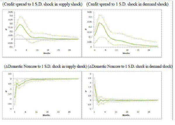
Figure 22: Historical decomposition of monthly growth in domestic non-core liabilities of the Korean banking sector (top panel) and the AA-corporate credit spread (bottom panel). The charts show the 12-month moving averages of identified demand and supply shocks on domestic non-core liabilities and the AA-corporate credit spread from contemporaneous impulse response in the VAR. Data are from the Bank of Korea.

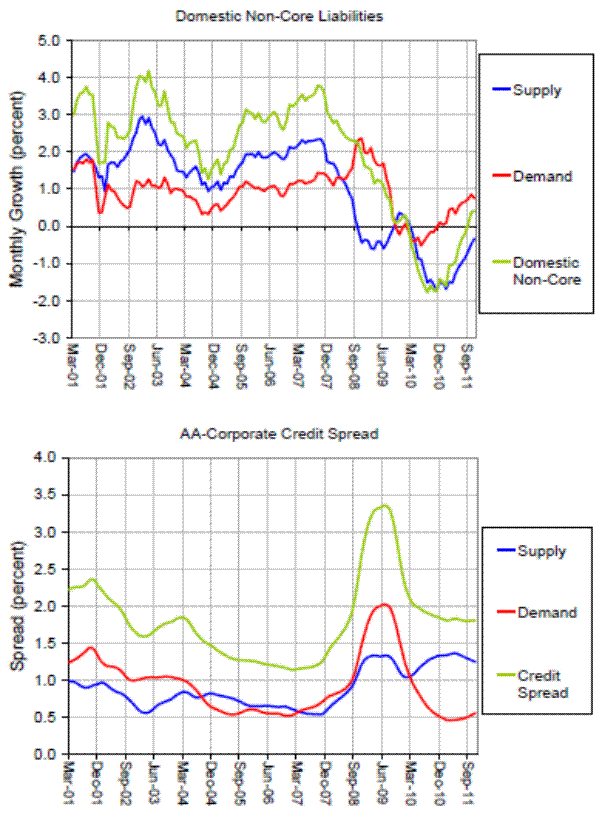
Figure 22 is the decomposition of the domestic non-core liabilities into supply-led and demand-led components, together with the decomposition of the AA-corporate bond spread into its demand and supply-led components.

There are some similarities in Figure 22 with the FX liabilities charts encountered earlier. For instance, we see that the upswing in the growth of domestic non-core liabilities before the Lehman bankruptcy of 2008 is supply-driven, but then in the late stage of the boom, the demand-led component takes over and perpetuates the boom right up to the crisis of 2008.

There are also some differences between the domestic non-core liabilities chart in Figure 22 from the FX liabilities chart in Figure 19. Notice also the dip in domestic non-core liabilities associated with the credit downturn following the asset losses experienced by domestic credit card companies in Korea. This downturn was mainly a domestically-driven event rather than the result of fluctuations in external liquidity conditions. Also, whereas the CIP spread decomposition identifies distinct supply-led and demand-led epochs during the sample period, the AA-corporate spread decomposition does not reveal any staggering of the supply and demand-led effects. In the bottom panel of Figure 22, we see that both the demand and supply-led components of the AA-corporate spread rise simultaneous with the onset of the Lehman crisis in 2008.

The difference between the FX liabilities charts and the domestic non-core charts is indicative of the external and internal dimensions of the financial crisis in Korea in late 2008, and further investigation may usefully reveal the reasons for the observed differences in time patterns.

5 Concluding Remarks

In this paper we have examined a conceptual framework that can serve to illuminate the relationship between some components of monetary aggregates and financial vulnerability. Since money is the balance sheet counterpart to bank lending, the most procyclical components of money correspond to the incremental lending at the peak of the financial cycle. As such, these procyclical components of money are most likely to be associated with bank lending that will reverse abruptly when the cycle turns. We have argued that cross-border banking sector liabilities to global banks exhibit the tell-tale procyclical patterns that can serve as such a signal. By monitoring the growth of such monetary aggregates as part of a comprehensive financial stability early warning system, the central bank may be able to gain valuable time in putting in place macroprudential policy measures that could lean agains the build-up of vulnerabilities.

In 2011, the Bank of Korea was granted the formal mandate for financial stability through the amendment of the law governing the Bank of Korea. This formal mandate offers both challenges and opportunities. An effective role in monitoring the financial system and the broader economy for signs of incipient vulnerabilities will need to rely on a systematic assessment of the potential channels of the propagation of financial instability.

In this paper, we have explored one possible component of the overall monitoring system. By tracking the procyclical components of monetary aggregates associated with cross-border banking sector liabilities, the central bank may gain valuable insights into the risk attitudes of the intermediary sector and the potential damage that may be done by an abrupt reversal of the permissive financial conditions that have fuelled the upswing. Through the instances of Korea and the eurozone, we have argued that a tell-tale sign of emerging vulnerability may be a prolonged period of rapid increase in monetary aggregates associated with cross-border banking. In this respect, we can see our results as providing further support to the cross-country finding in Hahm, Shin and Shin (2011) that the stock of FX banking sector liabilties is perhaps the most reliable indicator of the vulnerability to a financial crisis.

References

Adrian, Tobias, Paolo Colla and Hyun Song Shin (2012) "Which Financial Frictions? Parsing the Evidence from the Financial Crisis of 2007-9" working paper

Adrian, Tobias and Hyun Song Shin (2008) " Procyclical Leverage and Value-at-Risk" Federal Reserve Bank of New York Staff Report 338, http://www.newyorkfed.org/research/staff_reports/sr338.html

Adrian, Tobias and Hyun Song Shin (2010) " Liquidity and Leverage," Journal of Financial Intermediation, 19, 418-437

Baumol, William (1952) "The Transactions Demand for Cash: An Inventory Theoretic Approach" Quarterly Journal of Economics, 66, 545-56

Bernanke, Ben and Ilian Mihov (1998) "The Liquidity Effect and Long-Run Neutrality" Carnegie-Rochester Series on Public Policy, 49, 149-194.

Borio, Claudio and Piti Disyatat (2011) "Global imbalances and the financial crisis: Link or no link?" BIS Working Papers No 346 http://www.bis.org/publ/work346.pdf

Borio, Claudio, and Haibin Zhu (2008) "Capital Regulation, Risk-taking and Monetary Policy: A Missing Link in the Transmission Mechanism?" Bank for International Settlements Working Paper 268.

Brunner, Karl and Allan Meltzer (1976) "An Aggregate Theory for a Closed Economy" in Monetarism (ed) Jerome Stein, pp 69-103, North Holland, Amsterdam.

Brunnermeier, Markus and Yuliy Sannikov (2010) " The Theory of Money," working paper, Princeton University.

Chadha, Jagjit S. Luisa Corrado, and Qi Sun (2010) "Money and Liquidity Effects : Separating Demand from Supply" Journal of Economic Dynamics & Control, 34, 1732-1747.

Faust, Jon (1998) "The Robustness of Identified VAR Conclusions about Money" Carnegie-Rochester Series on Public Policy, 49, 207-244.

Friedman, Benjamin, M. (1988) "Lessons on Monetary Policy from the 1980s" Journal of Economic Perspectives, 2, 51-72

Friedman, Milton (1956) "The Quantity Theory of Money - A Restatement" in Studies in the Quantity Theory of Money (ed) Milton Friedman, Chicago University Press, Chicago.

Hahm, Joon-Ho, Frederic S. Mishkin, Hyun Song Shin, Kwanho Shin (2012) "Macroprudential Policies in Open Emerging Economies" NBER Working Paper No. 17780, January 2012 http://www.nber.org/papers/w17780.pdf

Hahm, Joon-Ho, Hyun Song Shin and Kwanho Shin (2011) "Non-Core Bank Liabilities and Financial Vulnerability" working paper

Hattori, Masazumi, Hyun Song Shin and Wataru Takahashi (2009) "A Financial System Perspective on Japan's Experience in the Late 1980s" Bank of Japan working paper, paper for BOJ conference, May 2009

Issing, Otmar (2003) "Monetary and financial stability - is there a trade-off?" paper presented at the BIS conference on "Monetary Stability, Financial Stability and the Business Cycle", http://www.bis.org/review/r030331f.pdf

Judd, John P. and John L. Scadding (1982) "The Search for a Stable Money Demand Function: A Survey of the Post-1973 Literature" Journal of Economic Literature, 20, 993-1023.

Miller, Merton and Daniel Orr (1966) "A Model of the Demand for Money by Firms" Quarterly Journal of Economics, 80, 413-435.

Peersman, Gert (2005) "What Caused the Early Millennium Slowdown? Evidence Based on Vector Autoregressions" Journal of Applied Econometrics, 20, 185-207.

Tobin, James (1956) "The Interest-Elasticity of Transactions Demand for Cash" Review of Economics and Statistics, 38, 241-47.

Tobin, James (1958) "Liquidity Preference as Behavior Towards Risk" Review of Economic Studies, 25, 65-86.

Tucker, Paul (2007) "Money and Credit: Banking and the Macroeconomy" speech given at the Monetary Policy and the Markets Conference, London, 13 December 2007 http://www.bankofengland.co.uk/publications/speeches/2007/speech331.pdf

Uhlig, Harald (2005) "What are the Effects of Monetary Policy on Output? Results from an Agnostic Identification Procedure" Journal of Monetary Economics, 52, 381-419.

Vasiceck, Oldrich (2002) "The Distribution of Loan Portfolio Value" Risk, December 2002, http://www.moodyskmv.com/conf04/pdf/papers/dist_loan_port_val.pdf

Footnotes

* Paper prepared for the Federal Reserve conference "Central Banking: Before, During, and After the Crisis" March 23-24, 2012. The views expressed in this paper are those of the authors and not necessarily those of the Bank of Korea. Return to Text

1. For a comprehensive survey of the demand for money, see Judd and Scadding (1982). See Friedman (1988) for the breakdown in the 1980s of the relationship between the money stock and macro variables. Return to Text

2. See Adrian and Shin (2010) for a more detailed study of the US investment banks. Return to Text

3. The $\lambda$ parameter for the HP filter is set at 14,400. Return to Text

4. The FX swap rate is $\log f_{t}$ - $\log S_{t}$ where $f_{t}$ and $S_{t\text{ \ }}$ are forward and spot USD/KRW exchange rates, respectively. It is annualized by multiplying it by four. Return to Text

^♣ This version is optimized for use by screen readers. Descriptions for all mathematical expressions are provided in LaTex format. A printable pdf version is available. Return to Text