
A Primer on the Macroeconomic Implications of Population Aging
Keywords: Population aging, social security, medicare, living standards
Abstract
The composition of the U.S. population will change significantly in coming decades as the decline in fertility rates following the baby boom, coupled with increasing longevity, leads to an older population. This demographic shift will likely have a dramatic effect on the long-run prospects for living standards. Moreover, as has been widely discussed in the media and by policymakers, population aging also has significant implications for social programs for the elderly, such as Social Security and Medicare.
In this paper, we discuss the consequences of population aging from a macroeconomic perspective and consider alternative paths the economy could follow in response to population aging. The choices society makes among those alternatives will be closely linked to decisions about how to reform entitlement programs for the elderly.
The fundamental conclusion of our study is that, barring a significant increase in labor force participation, population aging will lead to a reduction in per capita consumption relative to a baseline in which the demographic composition of the population does not change. The size of any consumption reduction depends critically on whether the adjustment happens sooner or later and on whether the labor force participation of the elderly changes. Important policy questions, then, are whose consumption path falls, by how much, when, and by what means? Decisions about Social Security and Medicare reform are integrally bound up with these fundamental policy questions.
I. Introduction
The composition of the U.S. population will change significantly in coming decades as the decline in fertility rates following the baby boom, coupled with increasing longevity, leads to an older population.1 This demographic shift will likely have a dramatic effect on the long-run prospects for living standards. Moreover, as has been widely discussed in the media and by policymakers, population aging also has significant implications for social programs for the elderly, such as Social Security and Medicare.
Much of the debate in recent years about Social Security has focused on financing issues--for example, on whether the program should continue to be financed solely through the current pay-as-you-go structure or whether personal accounts or other innovations should be introduced. The financing issues are important, but a deeper understanding of the underlying macroeconomic changes brought about by population aging may also be helpful.
In this paper, we discuss the consequences of population aging from a macroeconomic perspective and consider alternative paths the economy could follow in response to population aging. The choices society makes among those alternatives will be closely linked to decisions about how to reform entitlement programs for the elderly.
The second section of this paper reviews projections of the pivotal demographic variables and lays out the extent and contour of the coming demographic changes. Section III develops the analytic machinery necessary to gauge the macroeconomic effects of population aging. Section IV uses this machinery to provide stylized descriptions of plausible scenarios for standards of living (as measured by per capita consumption) as the population ages. Section V provides rough estimates of the magnitudes of the consumption adjustments that are likely to be required in coming years under several scenarios.
The fundamental conclusion of our study is that, barring a significant increase in labor force participation, population aging will lead to a reduction in per capita consumption relative to a baseline in which the demographic composition of the population does not change.2
- Assuming no increase in labor force participation among the elderly, one possible response to population aging would be to implement policies that cause the burden of reduced consumption per person to be shared equally across all generations. This would be achieved by reducing per capita consumption today to a path that would then be sustainable over time. Our simulations indicate that, in such a scenario, the required reduction in per capita consumption is about 4 percent relative to a baseline with unchanged demographics.3
- If the consumption adjustment is delayed by twenty years (and still assuming no increase in labor force participation), the required reduction in per capita consumption is estimated to be much larger, nearly 14 percent relative to baseline.
such large consumption adjustments, provided that most of the incremental increases in income are saved rather than consumed.
- If, for example, labor force participation among the elderly were raised today by boosting the age at retirement for all workers by two years, the required reduction in per capita consumption relative to baseline would be less than 1 percent.4
- If the retirement age were boosted by two years, but that change did not take effect for twenty years, and if the consumption adjustment did not occur for twenty years as well, then the required reduction in per capita consumption relative to baseline would be nearly 11 percent.
II. Demographic Projections
Many discussions of entitlement programs for the elderly focus on the expected decline in the ratio of the working-age population (persons aged 20 to 64 years) to the population of persons 65 years of age and older. For example, currently there are about 5 adults of working age for every person 65 and over, and the elderly constitute about 12 percent of the population. In 2030, by which time most of the baby boomers will have retired, the ratio is projected to be about three working-age adults per older person, and the elderly are expected to be about 19 percent of the population.5
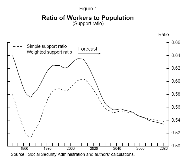
To gauge the macroeconomic effects of population aging, it is useful to focus on a different ratio--the ratio of the working-age population to the total population. This ratio highlights the number of potential workers available to support the entire population's consumption. In this paper, we refer to this ratio interchangeably as "workers per person" or as the "simple support ratio."6 However, a more accurate gauge of the effects of population aging on any person's consumption might weight the population by the consumption needs of different demographic groups. For example, the elderly may consume more than the non-elderly because of a greater need for medical care, so an increase in the proportion of elderly in the population may impose a greater strain on consumption than otherwise. Children, on the other hand, tend to consume much less than adults. The weighted support ratio is equal to the ratio of working-age adults to the weighted population.7
The historical and projected trends of the simple and the weighted support ratios are shown in figure 1. The weighted support ratio shows that future population aging will present a major economic challenge in the years ahead--far greater than that experienced in the 1960s and 1970s. Indeed, rather than temporarily dipping as it did in the earlier period, the weighted support ratio is projected to continue falling well beyond 2030, albeit at a much slower pace than during the earlier period, thus indicating that the population aging projected for the United States during this century is permanent and ongoing. The projected drop in both support ratios between now and 2080 stems from two factors: the decline in the fertility rate following the end of the baby boom in 1964 and an expectation of increasing longevity over the next century.8
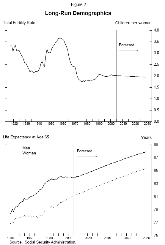
The fertility rate (the upper panel of figure 2) affects the support ratio because it determines the relative sizes of different age cohorts. Initially, the baby boom lowered the support ratio by increasing the number of children per worker. As these children entered the workforce and as the fertility rate fell, the support ratio rose. Finally, as the baby boomers enter retirement, the support ratio will fall to the level consistent with the current (and projected) fertility rate.9
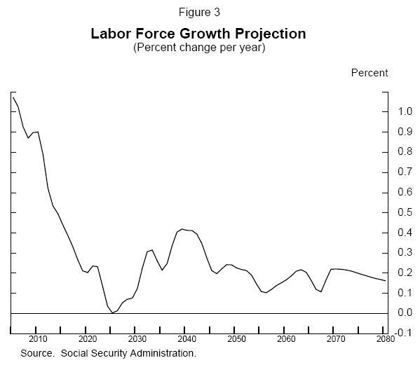
Besides affecting the support ratio, fertility affects the growth rate of the labor force: High fertility leads to a rapidly growing population and labor force; conversely, low fertility leads to a slowly growing or even shrinking labor force. As shown in figure 3, current projections are for the annual growth rate of the labor force to slow from about 1 percent currently to about 0.2 percent, on average, after 2020.
Longevity (the lower panel of figure 2) also affects the support ratio. In particular, increasing life expectancy at age 65 increases the number of older people in the population, raising the denominator of the support ratio.10 Unless longer life expectancy is accompanied by rising labor force participation among the elderly (an increase in the numerator), the support ratio will move down (holding fixed the fertility rate). Life expectancy is projected to continue increasing for the foreseeable future. The Social Security actuaries assume that life expectancy after age 65 will increase about 1/2 year per decade.
All else being equal, past and projected trends in fertility rates account for about two-thirds of the expected decline in the support ratio over the next 75 years, and the projected increase in life expectancy accounts for the remainder.
III. The Macroeconomic Consequences of Population Aging
As noted above, a primary conclusion of this paper is that population aging can be expected to lead to a decline in consumption per person relative to a baseline in which the population is not aging. To explore the connections between population aging and consumption per person, this section develops the machinery necessary to derive sustainable paths of consumption in the future, based on so-called consumption possibilities frontiers. This analytic apparatus is built from a series of identities and some central steady-state relationships from standard macro growth models.
The material in this section, the most technical in the paper, develops a relationship between consumption per person and capital per worker that can be used to gauge the effect of changes in fertility and longevity on consumption per person in a steady state (equation 5, below). As will be explained at the end of this section, figure 4 shows these relationships graphically.
The basic relationships
We start the analysis by examining how population aging affects output per person. The first thing to recall is that as the population ages, the support ratio--workers per person--decreases. This decrease means that for any given level of output per worker, the level of output per person falls. In a sense, each worker's output has to be shared with more people. This relationship is easily seen in equation 1:
(1) Output per person ![]() Output per worker * Workers per person,
Output per worker * Workers per person,
or
![]() ,
,
where ![]() is output,
is output, ![]() is population, and
is population, and ![]() is the labor force.
is the labor force.
Thus, for any given level of output per worker (that is, for any given level of labor productivity), as the number of workers per person declines, so too does output per person.
Although output per person is sometimes used as a measure of the standard of living, we use the measure that is often preferred by economists - namely, consumption per person. Consumption, of course, is the amount of output that is not saved. Thus,
(2a) Consumption per person ![]() Output per person - Saving per person,
Output per person - Saving per person,
or
![]() ,
,
where ![]() is consumption and
is consumption and ![]() is saving.
is saving.
Substituting equation 1 into equation 2a indicates that
(2b) Consumption per person ![]() Output per worker * Workers per person - Saving per person,
Output per worker * Workers per person - Saving per person,
or
![]() .
.
These expressions show that, in order to understand the effect of population aging on consumption per person, one must examine the effect of population aging on saving per person as well as the effect on output per person.
The analysis of saving per person relies on the notion from growth theory that, in steady state, a country's capital-labor ratio ![]() is constant. Accordingly, if the labor force
(
is constant. Accordingly, if the labor force
(![]() grows 10 percent, for example, then the country's capital stock (
grows 10 percent, for example, then the country's capital stock (![]() also must
grow 10 percent to keep the ratio constant as required for a steady state. But an increase in the capital stock must be matched by an equivalent amount of saving. In other words, if the labor force increases 10 percent, saving must be sufficient to increase the capital stock 10 percent.11 This steady-state requirement for the relationship between labor force growth
also must
grow 10 percent to keep the ratio constant as required for a steady state. But an increase in the capital stock must be matched by an equivalent amount of saving. In other words, if the labor force increases 10 percent, saving must be sufficient to increase the capital stock 10 percent.11 This steady-state requirement for the relationship between labor force growth ![]() and saving per worker is captured in equation 3a:
and saving per worker is captured in equation 3a:
(3a) Saving per worker = Capital per worker * Labor force growth rate,
or
![]() .12
.12
Multiplying both sides of (3a) by workers per person (![]() yields an expression in terms of saving per person:
yields an expression in terms of saving per person:
(3b) Saving per person =
Workers per person *[Capital per worker * Labor force growth rate],
or
![]() .
.
By substituting equation 3b into equation 2b, per capita consumption can be expressed as
(4) Consumption per person =
Workers per person * (Output per worker - Capital per worker * Labor force growth rate),
or
![]() .
.
Because the steady-state relationship between capital and labor (that is, a constant capital-labor ratio) has been inserted into the identity for consumption per person, equation 4 describes steady-state consumption per person.
Because of the linkage between saving and capital accumulation, on the one hand, and interest rates, on the other hand, it is useful to express equation 4 in a form that explicitly includes an interest rate term. We do this by re-writing the equation in terms of income rather than output. In
particular, the term for output per worker on the right-hand side of the equation can be expressed as wages per worker plus capital income per worker, where the latter is measured as the interest rate (the return to capital) times capital per worker.13 Hence, using ![]() as the total wage bill (labor income) and
as the total wage bill (labor income) and ![]() as the interest rate, consumption per person can be expressed as
as the interest rate, consumption per person can be expressed as
(5) Consumption per person =
Workers per person * (Wages per worker + r*Capital per worker - n*Capital per worker)
= Workers per person * (Wages per worker + (r-n) * Capital per worker),
or
![]() .
.
Equation 5 describes how steady-state consumption per person depends on workers per person (the support ratio), wages per worker, the capital-labor ratio, the interest rate, and the growth rate of the labor force. To analyze this relationship graphically, consumption per person typically is
plotted on the vertical axis and capital per worker on the horizontal axis. Such a plot shows steady-state or sustainable consumption per person for different levels of the capital-labor ratio holding constant workers per person ![]() , wages per person
, wages per person ![]() , the interest rate
, the interest rate ![]() and labor force growth
and labor force growth ![]() . However, before plotting equation 5, we must deal more fully with the manner in which saving, investment, and capital per worker are linked to
the interest rate, or return to capital.
. However, before plotting equation 5, we must deal more fully with the manner in which saving, investment, and capital per worker are linked to
the interest rate, or return to capital.
Saving and interest rates
The relationship between saving, capital per worker, and the return to capital depends on whether the economy is best described as one in which changes in domestic saving affect domestic interest rates or as one in which changes in saving do not affect interest rates. Standard terminology describes these two possibilities, respectively, with the nomenclature "closed economy" and "small open economy," and we will use these labels.
In a closed economy, domestic saving and investment are identical, because all domestic saving is invested in domestic capital and all capital is financed only with domestic saving. In this economy, increases in saving (investment) raise the domestic capital-labor ratio. The higher capital-labor ratio increases labor productivity, resulting in higher wages; but the extra capital associated with the higher saving lowers the return to capital (the interest rate).14
At the other extreme, an economy might be described as a small open economy. In this type of economy, interest rates are set on the global market and are unaffected by domestic saving, which may be invested at home or abroad. As a result, increases in domestic saving do not affect the capital-labor ratio, wages, or the return to capital.
Neither of these models perfectly describes the United States. However, some basic facts and empirical work suggest that the closed economy case is a better approximate description of the U.S. economy. Namely, net capital flows are small relative to the size of the capital stock, and a range of empirical work suggests that changes in domestic saving do affect interest rates. On the other hand, the U.S. economy has trade and financial links with the rest of the world, which have become increasingly important over time. Indeed, net capital flows into the United States, which averaged between 1 and 2 percent of GDP during most of the 1990s, have shot up to more than 6 percent of GDP recently. It is conceivable that, over the next several decades, the direction of the flows could reverse, with large amounts of U.S. capital possibly going to developing countries; if this were to occur, the United States would be able to save more without depressing the rate of return.15
Because of these two possibilities, we simplify the discussion in the text by focusing on the closed economy case, in which changes in saving do affect rates of return. We model cases for a small open economy in the appendix. When we model the United States as an open economy, we substitute the concept of assets per worker for that of capital per worker and hold the return to assets constant as assets per worker increase.
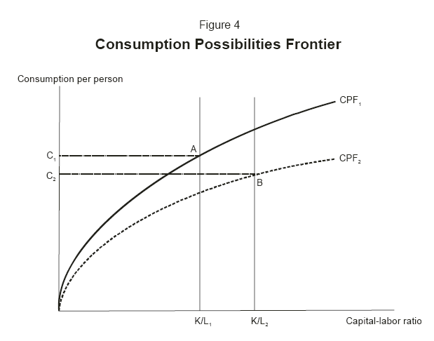
The consumption possibilities frontier
As noted earlier, equation 5 can be plotted holding constant workers per person, wages per worker, the labor force growth rate, and the interest rate to show how consumption per person varies as the capital-labor ratio changes. We call this relationship the consumption possibilities frontier (CPF). The solid line in figure 4 plots a typical CPF drawn for a closed economy. As the capital-labor ratio increases, consumption per person rises. But the increment to consumption gets smaller for each additional increase in the capital-labor ratio, causing the CPF to begin to flatten. Why does this occur? Recall from equation 4 that consumption per person depends on output per person. With declining marginal returns, the marginal increase in output per person from increases in the capital-labor ratio diminishes as the capital-labor ratio rises.
How does population aging affect the CPF? An increase in longevity reduces the ratio of workers per person. The reduction in workers per person (the ![]() term in equation 5) shrinks
consumption per person at every level of capital per worker. A reduction in the fertility rate not only has this effect but also reduces labor force growth. The drop in labor force growth (which enters equation 5 with a negative sign) tends to push up consumption per person.16 For the United States, as it turns out, the effect of the drop in workers per person outweighs the effect of slower labor force growth, so that the net effect of population aging is
a reduction in consumption per person for any given level of capital per worker. Graphically, this is depicted in figure 4 by the dashed line, which pivots down relative to the solid line.
term in equation 5) shrinks
consumption per person at every level of capital per worker. A reduction in the fertility rate not only has this effect but also reduces labor force growth. The drop in labor force growth (which enters equation 5 with a negative sign) tends to push up consumption per person.16 For the United States, as it turns out, the effect of the drop in workers per person outweighs the effect of slower labor force growth, so that the net effect of population aging is
a reduction in consumption per person for any given level of capital per worker. Graphically, this is depicted in figure 4 by the dashed line, which pivots down relative to the solid line.
With this machinery in hand, we can now provide a richer description of the macroeconomic effects of population aging.
IV. The Effects of Population Aging on the Macroeconomy: A Stylized Description
The analysis thus far has shown how population aging shifts the consumption possibilities facing the economy.17 In particular, equation 2b shows that population aging reduces per capita consumption relative to a baseline without population aging. But equation 5 shows that a lot of moving parts are embedded in equation 2b, reflecting the complex interactions among saving, interest rates, capital accumulation, and labor force growth. Moreover, equation 5 describes only steady states--that is, the ultimate levels of per capita consumption associated with a demographic change. It does not say anything about the transition path from one steady state to another or about where along the new frontier the economy will end up. Indeed, an infinite number of transition paths are possible, and any point along the frontier is possible. In this section, we describe how the moving parts of equation 5 affect the transition path and the ultimate steady state using one particular transition path as an expository example.
The effects of changes in the fertility rate
Using figure 4, we present a stylized description of what happens as changes in the fertility rate alter the CPF and the economy moves from one steady state to another.18 As discussed previously, a reduction in the fertility rate causes the consumption possibilities frontier (CPF) to shift down. The transition path from the initial CPF to the new CPF can be pinned down by assumptions about two related factors: 1) how long consumers wait before beginning the transition to the new steady state and 2) how different generations bear the burden of the adjustment. Choices about how long to wait and how to share the burden will be determined by societal preferences as reflected in individual and governmental decisions about saving and consumption. For this stylized description, we assume that the change in demographics occurs in the future but that the transition begins immediately. We also assume that the required consumption adjustment is shared equally (in percentage terms) by the current and all future generations. Both of these assumptions are critical to the example presented here. If either assumption is altered, the economy will follow a different transition path and will end up with a different steady-state level of per capita consumption. Nevertheless, the basic analytics are the same.
Although this discussion provides some basic intuition about the effects of a reduction in fertility, it addresses only some of the complexities in order to keep the analysis reasonably tractable. In particular, we do not discuss the "exogenous" (that is, nonbehavioral) change in the capital-labor ratio associated with a drop in the fertility rate--namely, as the labor force decreases, the capital-labor ratio automatically increases even without any reduction in consumption.19 We omit this capital intensity effect from the discussion because the exogenous increase in the capital-labor ratio associated with a drop in fertility is not the steady-state change in the ratio. Nevertheless, it should be kept in mind that the capital intensity effect tends to damp somewhat the size of the ultimate consumption adjustment.20
To simplify the exposition, we assume that shifts in the CPF occur instantaneously, rather than over decades. In addition, we present the analysis as if events transpire sequentially. In fact, a number of adjustments will be taking place simultaneously over an extended period of time. 21 Moreover, the stylized picture and description abstract from growth in multifactor productivity and ongoing trend growth in consumption per capita. Thus, even though the picture suggests an absolute decline in consumption per capita, in actuality, the analysis merely indicates that consumption per capita in the new steady state is lower than it would have been in the absence of population aging.
The analysis begins with the economy in steady state at point A on figure 4. At that point, the economy has a capital-labor ratio of K/L![]() and per capita consumption of C
and per capita consumption of C![]() . The reduction in the fertility rate causes a shifting down in the CPF from CPF
. The reduction in the fertility rate causes a shifting down in the CPF from CPF![]() to
CPF
to
CPF![]() . After the shift in the CPF, consumption would not be sustainable at C
. After the shift in the CPF, consumption would not be sustainable at C![]() because at such a level saving and investment would be too small and the relative size of the capital stock would begin to shrink. In effect, the economy would be consuming its capital. To prevent such an outcome, per capita consumption must fall.
because at such a level saving and investment would be too small and the relative size of the capital stock would begin to shrink. In effect, the economy would be consuming its capital. To prevent such an outcome, per capita consumption must fall.
If the necessary adjustment to consumption per capita occurs immediately, how much must consumption fall so that the burden of the adjustment is shared equally by the current and all subsequent generations? The reduction in per capita consumption must be large enough so that, if this level of
consumption is maintained for all time, the economy will generate exactly the amount of saving and investment required to raise the capital-labor ratio to a point on CPF![]() at which this
level of per capita consumption can be sustained. In the figure, this required level of per capita consumption is C
at which this
level of per capita consumption can be sustained. In the figure, this required level of per capita consumption is C![]() , which places the economy at the new steady state, denoted as "B," on
CPF
, which places the economy at the new steady state, denoted as "B," on
CPF![]() .
.
Point B is unique given the shape of the consumption possibility frontier, the magnitude of the population-aging shift, and the assumptions made about the timing of the consumption shift and the intergenerational sharing of the burden. A level of per capita consumption greater than C![]() would generate too little saving and investment, and K/L would move to the left indefinitely; per capita consumption less than C
would generate too little saving and investment, and K/L would move to the left indefinitely; per capita consumption less than C![]() would generate too much saving, and K/L would move to the right indefinitely. More generally, any combination of assumptions about the timing of the consumption adjustment and generational burden sharing will produce a unique steady state.22
would generate too much saving, and K/L would move to the right indefinitely. More generally, any combination of assumptions about the timing of the consumption adjustment and generational burden sharing will produce a unique steady state.22
The effects of increases in longevity
From a microeconomic perspective, as people live longer, they need either to work longer or to consume less.23 From a macroeconomic perspective, increases in longevity increase the elderly population but (assuming no change in labor force participation by age) have no effect on the number of workers or the growth rate of the labor force. Thus, their only effect is to lower the ratio of workers to the population, causing the consumption possibilities frontier to shift down. Exactly where the economy ends up on the new consumption possibilities frontier depends on public policy and on the tradeoffs people make between consumption during their working years and consumption during their retirement. For example, a purely private response to increased longevity would likely involve saving more when young--either by consuming less, working more, or both--thus boosting the capital-labor ratio, and then consuming the pre-retirement savings during retirement.
Intergenerational links
The story presented thus far has glossed over a critical aspect of the economics of population aging--that is, the links between generations. If generations were not linked, then, by definition, the consumption choices of one generation and the generation's size would not affect the consumption possibilities of subsequent generations. But intergenerational linkages are important. Such linkages include not only transfer programs and bequests but also, in a closed economy, connections through saving and the return to capital. These intergenerational links mean that decisions about consumption and saving (for example, with regard to funding Social Security) that were made by earlier generations affect the consumption and saving possibilities for current and future generations. Similarly, the response of today's generation to population aging (for example, when and how much to reduce their consumption path) directly affects subsequent generations.
The presence of links through transfer programs and bequests is obvious; the link through the effect of saving on the return to capital is more subtle. Consider, for example, an economy with no bequests or pay-as-you-go transfer programs, so that each individual saves for his or her own
retirement. In a closed economy, a decrease in the fertility rate lowers the relative size of the labor force and boosts capital per worker.24 But because of the assumed
declining marginal product of capital, the increase in capital per worker lowers the return to saving ![]() . The drop in the return to saving permanently reduces the flow of capital income
(rK), which forces a change in consumption not only for the current generation but also for future generations. Thus, in a closed economy, even without transfer payments or bequests, a decline in the fertility rate today would affect the consumption possibilities of future
generations.25
. The drop in the return to saving permanently reduces the flow of capital income
(rK), which forces a change in consumption not only for the current generation but also for future generations. Thus, in a closed economy, even without transfer payments or bequests, a decline in the fertility rate today would affect the consumption possibilities of future
generations.25
Entitlement programs and consumption possibilities
The creation and the presence of entitlement programs for the elderly such as Social Security and Medicare, by transferring income from one generation to another, influence society's consumption and saving choices and, therefore, the size of the capital stock and the capital-labor ratio. For example, early participants in Social Security paid little in contributions relative to the benefits they received when they retired. As a result, this earlier generation's rate of capital accumulation and the current capital-labor ratio are lower than they would have been had the program been fully funded at the start. This outcome is what might be thought of as the "legacy cost" of a pay-as-you-go system. In addition, the ongoing presence of entitlement programs for the elderly affects private consumption and saving choices today, with implications for future consumption possibilities. These issues are explored further in an appendix, which compares paths of steady-state per capita consumption in an economy having intergenerational transfers with such paths in an economy not having intergenerational transfers.
Another way that these entitlement programs influence consumption possibilities is by specifying rules for transfers between generations. For example, the current Social Security law would sustain benefit payments to the elderly under the current formula until the trust fund is exhausted in 2040 (as projected by the Social Security trustees). At that time, under current law, benefits would be reduced to bring them into line with incoming payroll taxes. This pattern of transfers is incompatible with the equal sharing of the burden of population aging across generations that was described in figure 4; instead, the current generation of retirees would avoid any reduction in consumption. Such an outcome may be inconsistent with societal preferences and views of fairness. Thus, achieving financial balance in these entitlement programs is really about deciding how the burdens of population aging will be shared across generations.
V. Empirical Magnitudes for the U.S. Economy
The previous section provided some intuition for why population aging matters economically. In this section, we analyze the likely magnitudes of the changes in the consumption possibilities frontiers in the United States and discuss possible responses to population aging.
To calibrate the analytic framework to features of the U.S. economy and demographics, we need to account for some additional factors. First, the demographic shocks in coming decades are more complicated than the simple one-time shocks depicted above. To account for this complexity, we use the intermediate projections from the Social Security actuaries.
Second, we add in the factors of depreciation and technical progress, which the previous discussion omitted.26 We assume that technical progress boosts growth 1.4 percent per year and that depreciation is 6 percent per year.27 Finally, we use a weighted support ratio that reflects the different consumption needs of the youth, adult, and elderly populations. 28
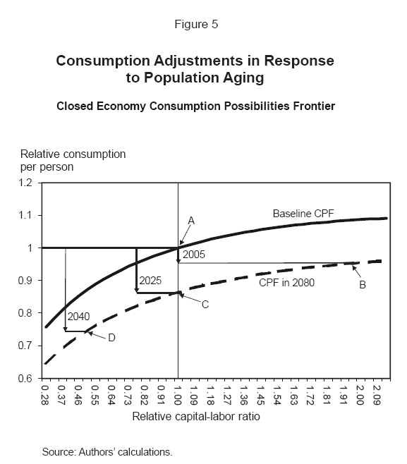
With these extensions to the framework, we use figure 5 to show consumption possibilities frontiers calibrated to the U.S. economy and demographics under the assumption that the United States is a closed economy.29 The figure is scaled relative to a baseline case in which the current growth rate of the labor force and the current support ratio are assumed to be unchanged in the future. Consumption per person (CPP) on the vertical axis is indexed to 1 at the baseline level of steady-state CPP.30 On the horizontal axis, the capital-labor ratio is indexed to 1 at the level associated with baseline steady-state CPP.
The solid line in figure 5 shows the baseline consumption possibilities frontier. The dashed line shows the CPF under the demographic structure that is projected for 2080, assuming that the economy has reached steady state in 2080. Reflecting the scaling system used for the figure, the dashed line, in effect, plots relative consumption per person (relative to a baseline in which the demographic structure does not change).
Possible consumption paths for the United States
The consumption possibilities frontiers in figure 5, like those in figure 4, show only steady states. Moreover, as mentioned previously, an infinite number of paths could eventually lead to the new long-run steady-state frontier. The path society chooses will depend on private preferences about consumption and saving as well as on the government response to population aging. The crucial policy question is how this reduction in consumption will be apportioned across groups and over time, and answers to that question will depend critically on societal views of fairness and on the tradeoffs between consumption at different times.
To pin down an optimal transition path, one would have to specify individual preferences and the government's policy choices. In lieu of tackling that very challenging problem, we illustrate several possible (though not necessarily optimal) consumption trajectories to assess the rough magnitude of the consumption adjustments required in the United States and the tradeoffs between making changes to consumption sooner and making them later. Using the analytic framework developed above, we simulate consumption trajectories that take us from our current demographic structure and capital-labor ratio to a new steady state consistent with the projected demographics in 2080.31
Sharing the burden equally across generations. As discussed in the stylized example, one possible response to population aging might be to reduce consumption per person today to a level that would then be sustainable over time--that is, to a level that could then grow at the rate of technical progress even as the population ages.32 This response would equalize the burden of population aging across generations because each member of each generation would suffer the same percentage decline in per capita consumption relative to baseline. However, nothing is sacrosanct about such a pattern: Different perspectives on fairness would lead to arguments in favor of different patterns of consumption across time. Nonetheless, this scenario provides a useful baseline for gauging the required adjustments to consumption.
How much would consumption per person have to fall today to place it on a sustainable path--that is, growing at the rate of technical change as the population ages? If the United States economy is modeled as a closed economy, the required reduction in per capita consumption is about 4.4 percent.33
Delaying the consumption response. If instead of reducing per capita consumption today, we maintain it at its current level for a time (actually allowing it to grow from its current level at the rate of technical change), how much will consumption per person ultimately need to fall? As shown in table 1, the greater the delay in reducing per capita consumption, the greater will be the reduction required to reach a new steady state on the consumption possibilities frontier consistent with the projected U.S. demographics over the next seventy-five years.
| Year adjustment begins | Percentage change in real per capita consumption required relative to 2005 baseline |
|---|---|
| 2005 | -4.4 |
| 2015 | -6.8 |
| 2025 | -13.7 |
| 2040 | -26.9 |
Note: We assume that the demographic variables are constant after 2080 and that the economy is closed.
Figure 5 shows a schematic of the economy's path under some of the alternatives, assuming a closed economy. In the case of the immediate reduction in consumption, per capita consumption falls nearly 4-1/2 percent today, and the capital-labor ratio grows until it reaches its new steady state at point B, which has a capital-labor ratio about two times larger than today's. Suppose instead, that current consumption is maintained for twenty years (that is, until 2025). In such a circumstance, saving would be inadequate relative to labor force growth, and the capital-labor ratio would drop 25 percent. When the necessary adjustment finally begins in 2025, consumption drops nearly 14 percent, and the capital-labor ratio begins increasing until it reaches its new steady-state value at point C, about the same as today's. If per capita consumption is maintained at current levels through 2040 despite the large demographic changes, consumption would have to drop almost 27 percent, and the capital-labor ratio, after falling to less than one-half the current level, would edge up to a steady-state value equal to about one-half its current level at point D.
Raising labor force participation
An alternative to reducing consumption is to raise output by increasing labor force participation. (Of course, an increase in labor force participation can be viewed as a decrease in the consumption of leisure.) Higher participation raises consumption possibilities by boosting the number of workers relative to the population. To determine the extent to which increased labor force participation could affect steady-state consumption, we present the results of simulations with higher labor force participation by the elderly. In the previous simulations, we modeled the workforce as proportional to the adult population aged 20 to 64. In these simulations, we examine the effects of including older adults as workers by modeling the workforce as proportional to the size of the adult population including older adults. As a technical matter, we do this by increasing the size of the labor force by a factor equal to the size of the population of added older adults (for example, the size of the population aged 65 and 66) relative to the size of the population aged 20 to 64. Using 2005 values, adding those aged 65 and 66 is equivalent to increasing the size of the labor force by 2.4 percent.
Exactly how such an increase in the size of the labor force could be accomplished is unclear. In all likelihood, a rise in participation rates for workers aged 55 and over would be necessary. An increase of this magnitude would probably require major adjustments to both business and government policies. For example, businesses could re-structure their operations to include more opportunities for part-time or flexible work schedules, which are often appealing to older workers, or the government could make adjustments to such things as the age at which workers are first entitled to receive Social Security benefits (the early retirement age) and the age at which they are eligible to receive Medicare as well. For expositional simplicity, we refer to these and similar types of policies as raising the retirement age.
As table 1 shows, with no change in elderly labor force participation, consumption would have to fall 4.4 percent below baseline if the consumption adjustment were to take place immediately. A 20-year delay in the consumption adjustment would increase the amount that consumption would need to decline, to 13.7 percent. Table 2, line 1, reproduces that information. The remainder of table 2 indicates how greater participation in the labor force by the elderly affects the required adjustment in consumption.
Table 2
Steady-state Consumption Adjustments with
Higher Elderly Labor Force Participation:
Required change in real per capita consumption relative to 2005 baseline (percent)
| Immediate adjustment in consumption | Adjustment in consumption in 2025 | |
|---|---|---|
| 1.Retire at age 65 | -4.4 | -13.7 |
| Immediate adjustment in consumption | Adjustment in consumption in 2025 | |
|---|---|---|
| 2. Retire at age 67 | -0.7 | -1.5 |
| 3. Retire at age 70 | +4.3 | +7.7 |
| Immediate adjustment in consumption | Adjustment in consumption in 2025 | |
|---|---|---|
| 4. Retire at age 67 | -2.7 | -10.8 |
| 5. Retire at age 70 | -1.3 | -6.7 |
As shown on line 2, an immediate increase in the retirement age from 65 to 67 would suffice to offset most of the effects of population aging: If the consumption adjustment takes place immediately, the required reduction is less than 1 percent; if it is delayed twenty years, the required reduction is 1.5 percent.34 As noted previously, these simulations require that the incremental increases in output be mostly saved. If instead, as people work longer and earn more, they also raise their consumption significantly, then the benefits of higher elderly labor force participation for steady-state consumption will be much smaller.35 Finally, as shown on line 3, an immediate increase in the retirement age to 70 would be more than enough to offset the effects of aging and would allow consumption to increase considerably.
An increase in the labor force participation of 65 and 66 year olds is unlikely to occur in such a fast and sharp manner. To get an idea of the effects of a less rapid increase in labor force participation, we analyze the effects of delaying the increase for twenty years. As shown in table 2, line 4, with a twenty-year delay, increasing the retirement age from 65 to 67 is not as effective at offsetting the effects of population aging. If consumption drops immediately, the required reduction is 2.7 percent; if the consumption adjustment is also delayed twenty years, the required reduction (in twenty years) is almost 11 percent.36 Even raising the retirement age to 70--line 5--is insufficient to offset all the consumption effects of population aging when the increase in labor force participation is delayed.
Caveats
Our analysis has focused only on population aging and has ignored a number of other factors that may affect the size of the required adjustment in per capita consumption. First, our analysis assumes that the economy is in steady state, given today's demographics. In such a steady state, the current level of consumption would be sustainable if the support ratio and labor force growth rate were not changing. However, the economy may not currently be in steady state, and current consumption may be too high, even with today's demographics. For example, the personal saving rate is very low, and the national saving rate also is quite low by historical standards. Moreover, the United States has run large current account deficits in recent years, financed by foreign borrowing. Accordingly, many commentators have argued that saving is inadequate in the United States. However, nailing down that widely held presumption is a formidable task. Calculations about the optimality of consumption and saving are difficult, requiring assumptions about the social rate of time preference (a discount rate) and the social intertemporal elasticity of substitution (capturing the degree to which society's preferences are egalitarian across generations).37 Similarly, identifying the optimal current account balance is quite challenging; and in some circumstances, borrowing from abroad would be optimal.
Another factor that we omitted is the effect of continuing rapid increases in health care costs. In our analysis, we account for the fact that, because of greater spending on health care, the elderly consume more total resources than the non-elderly. But we assume that, for the future, consumption weights by age group will be constant, implying that any increases in elderly health spending are offset by reductions in elderly nonhealth spending. If society instead chooses to spread the burden of higher elderly health spending across different age groups, then increases in health care spending will raise the consumption of the elderly relative to the non-elderly and require a larger cutback in non-elderly spending than implied by the numbers in our analysis.38
Another factor that could affect the size of the needed adjustment in consumption is the possible endogeneity of technological progress. We assumed that the rate of technological progress is fixed, but technological progress may be endogenous with respect to population aging. A slowdown in the growth rate of the labor force could spur productivity gains as firms are forced to develop new labor-saving modes of production. With productivity growth faster than in our simulations, the necessary adjustment in consumption would be smaller. However, to the extent that innovation is linked to flexible thinking, an older society may be a less innovative society. And as Ellwood (2001) argues, current demographic projections suggest that rates of increase in educational attainment are likely to slow in the future, providing another possible source of drag on labor productivity growth. With productivity growth slower than in our simulations, the necessary adjustment in consumption would be larger.
VI. Conclusion and Policy Implications
Absent a sizable increase in labor force participation, the demographic transition we are about to undergo in this country will require a reduction in per capita consumption relative to what it could have been in the absence of demographic change. Given this basic fact, the main macroeconomic policy questions for the nation are (1) How much can we (and should we) raise labor force participation? and (2) How do we want to allocate the burden of reduced consumption over time? Implicitly, every proposal to reform entitlement programs for the elderly must provide an answer to these two questions; and the proposals can be compared on that basis.
We close with some comments on solvency of Social Security in the context of the analytical framework presented above. Social Security is solvent if the present value of future tax revenues plus current assets is equal to the present value of future benefits. Today, of course, the system is not solvent. The insolvency occurs, in large part, because of the population aging described in this paper--specifically the decline in the support ratio (the number of workers per person). Dealing with this financing problem can be seen as providing part of the answer to the larger questions about the timing and size of consumption adjustments.
For example, Social Security could become solvent by cutting benefits or raising taxes or both in the future or by cutting benefits or raising taxes or both now. These two macroeconomic policies are very different in the sense that the former allows consumption to stay at current levels now but significantly reduces future consumption, whereas the latter begins the consumption adjustment now, requiring less of an adjustment later. Thus, reform plans intended to achieve solvency should be evaluated in terms of whose consumption path is lowered and when and by how much it is cut.39
This discussion emphasizes that the question of how to deal with the problem of achieving financial balance in entitlement programs for the elderly cannot be divorced from the basic question of how society responds to population aging. The choices made will determine how the burden of population aging is shared within and across generations.
REFERENCES
Cohen, Darrel, Kevin Hassett, and Jim Kennedy (1995). "Are U.S. Investment and Capital Stocks at Optimal Levels?" Finance and Economics Discussion Series 199532. Washington: Board of Governors of the Federal Reserve System, July.
Ellwood, David T. (2001). "The Sputtering Labor Force of the Twenty-first Century: Can Social Policy Help?" in Alan Krueger and Robert Solow, eds., The Roaring Nineties: Can Full Employment Be Sustained? New York: Russell Sage Foundation, pp. 421-89.
Elmendorf, Douglas W., and Louise M. Sheiner (2000a). "Should America Save for Its Old Age? Population Aging, National Saving, and Fiscal Policy," Finance and Economics Discussion Series 2000-03. Washington: Board of Governors of the Federal Reserve System, August.
Elmendorf, Douglas W., and Louise M. Sheiner (2000b). "Should America Save for Its Old Age? Fiscal Policy, Population Aging, and National Saving," Journal of Economic Perspectives, vol. 14 (Summer), pp. 57-74.
Follette, Glenn, and Louise Sheiner (2005). "The Sustainability of Health Spending Growth," National Tax Journal, vol. 58 (September), pp. 391-408.
Appendix: Illustrative Examples Highlighting the Channels through Which Population Aging and Social Security Affect Consumption and Saving
The effects of a reduction in fertility on consumption are more complex than discussed in the main body of the paper. Indeed, in one particular case, a drop in the fertility rate would have no effect on sustainable consumption per capita. To illustrate more fully the circumstances under which changes in the fertility rate would matter for consumption, we present some illustrative examples of different cases in this appendix.
In the main text, we assumed a closed economy because that assumption probably provides a better description of the U.S. economy than the small, open-economy assumption. Here, we assume an open economy because that assumption provides a more straightforward mechanism for highlighting the importance of intergenerational links. In particular, we show that, in an open economy without intergenerational links, changes in fertility have no effect on sustainable consumption because the "exogenous" increase in the asset-labor ratio brought on by a reduction in the fertility rate (the capital intensity effect) is just large enough to offset the effects of the shift of the consumption possibilities frontier. (It is important to recall that only an open economy can have no intergenerational linkages; as discussed previously, the dependence of the rate of return to saving on the capital-labor ratio in a closed economy necessarily creates intergenerational links.) We then illustrate that, when intergenerational transfers are introduced, sustainable consumption is affected by changes in fertility.
In the first example, we consider a drop in fertility in an economy with no intergenerational links--that is, a small open economy with no transfer programs, such as Social Security. In the second example, we consider the effect of a drop in fertility in a small open economy with a social security system that creates intergenerational links. We show that, in this economy, a reduction in the fertility rate is no longer neutral and, indeed, requires consumption to fall.
These examples are useful for two reasons. First, they provide additional intuition about why changes in fertility affect consumption possibilities. Second, they highlight how the presence of transfer programs like Social Security affect consumption and saving choices.
Decline in the fertility rate, no intergenerational links
We consider an economy in which people live for two periods. In the first period they are working adults, and in the second period they are retired.40 People save for their retirement while working and consume their assets when retired. As table A.1, line 1, shows, we assume that the wage rate is $100 and the interest rate is 133 percent (think of each period lasting many years, line 2). The fertility rate in the first period is 4 (line 3). Because each woman has four children, the number of young people is twice the number of old people (lines 4 and 5), and the labor force doubles every period (line 6). In the second period, the fertility rate drops to 2, so that the number of young equals the number of elderly, and the labor force growth rate drops to 0.
Lines 7-11 describe the consumption and saving decisions. Assuming that people want to maintain constant consumption throughout their lifetime, each person will consume $70 in the first period and save $30. By the beginning of the second period, their assets will be $70 (saving of $30 plus interest income of $40 [$30*1.33]), which they will use to finance retirement consumption. Saving in the second period is equal to $30 (second period income of $40 less second period consumption of $70).
As this example shows, no individual choices are affected by population aging-consumption remains unchanged, and saving remains unchanged. There are, however, changes in the macroeconomic variables.
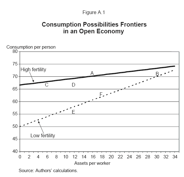
The consumption possibilities frontiers for this economy appear in figure A.1. Because wages and the interest rate are fixed (the open economy assumption), the consumption possibilities frontiers are straight lines. As shown in the main text, the consumption possibilities frontier is defined as
Consumption per person = Workers per person * (Wages per worker + (r-n) * Assets per worker).
Plugging in the values from these examples, the consumption possibilities frontiers (CPFs) are
High fertility CPF: 200/300*(100 + (1.33-1) * AW) = 66.7 + .20*AW, and
Low fertility CPF: 200/400*(100 + (1.33-0) * AW) = 50.0 + .65*AW,
where AW is assets per worker. As can be seen, population aging reduces the intercept term for the CPF and increases the slope term.
Over the range of values relevant for the United States, the new CPF (the dashed line) lies below the original CPF. Consequently, at any given level of assets per worker, consumption possibilities are lower. So, how does this mesh with the fact that consumption per person does not change?
The key is that assets per worker, shown on line 18 of table A.1, increases from $15, point A in figure 6, to $30, point B in the figure. With this "exogenous" increase in assets per worker (exogenous in the sense that it derives from changes in demographics, not changes in consumption or saving behavior), consumption per person does not have to change.
Table A.1
Decline in Fertility with No Intergenerational Links
| Period 1 | Period 2 | |
|---|---|---|
| 1. Wage rate | $100 | $100 |
| 2. Interest rate | 133% | 133% |
| Period 1 | Period 2 | |
|---|---|---|
| 3. Fertility rate | 4 | 2 |
| 4. Number young | 200 | 200 |
| 5. Number old | 100 | 200 |
| 6. Labor force growth rate | 100% | 0% |
| Period 1 | Period 2 | |
|---|---|---|
| 7. Per capita consumption | $70 | $70 |
| 8. Saving of young | $30 | $30 |
| 9. Dissaving of old | -$30 | -$30 |
| 10. Income per young person | $100 | $100 |
| 11. Income per old person | $40 | $40 |
| Period 1 | Period 2 | |
|---|---|---|
| 12. Income | $24,000
(200*$100 + 100*$40) |
$28,000
(200*$100 + 200*$40) |
| 13. Assets | $3,000
(100*$30) |
$6,000
(200*$30) |
| 14. Saving | $3,000
(200*$30 - 100*$30) |
$0
(200*$30 - 200*$30) |
| Period 1 | Period 2 | |
|---|---|---|
| 15. Income | $80
($24,000/300) |
$70
($28,000/400) |
| 16. Saving | $10
($3,000/300) |
$0 |
| 17. Consumption | $70 | $70 |
Decline in fertility with a social security system
This example adds a social security system. The economic and demographic variables are the same as in the previous example. The social security tax rate is 20 percent (table A.2, line 7). In the first period (before the demographic shock), the total taxes collected are $4,000 ($20*200), which provides a benefit of $40 per old person, line 8. In the second period (after the decline in fertility), social security tax collections are still $4,000, but there are twice as many retirees, bringing the benefit down to $20 per old person.
Lines 9 through 14 report the consumption, saving, and income of the young and the old. As in the first example, consumers want to smooth consumption throughout their lifetime. However, the existence of the social security system lowers consumption--it is $68 in the first period, whereas it was $70 in the previous example--because the rate of return on social security is 100% (a tax of $20 yields a benefit of $40) rather than the 133% available in the private market.
Also, unlike the first example, consumption now depends on the fertility rate, because the social security benefit changes with the ratio of workers to retirees. In this example, the period 2 decline in fertility is unforeseen in period 1. Thus, young workers in period 1 do not adjust their consumption or saving. As a result, in period 2, these workers, now retirees, have much lower consumption because benefits fall from $40 to $20. In the third period, the new steady state, consumption is $62.
As in the first example, assets per worker--line 21--double in response to population aging. But, in this case, assets per worker started off at only $6, point C in figure A.1, and a doubling of assets per worker--to point D, is insufficient to allow consumption to remain unchanged.41 In this example, the adjustment to the new steady state takes place over two periods. Consumption in period 2 is marked as E--a bit below the new CPF, raising assets per worker and bringing the new steady-state consumption point to point F.
While this example is highly stylized, it does provide intuition about the important role of intergenerational links in the macroeconomic consequences of population aging.
Table A.2
Decline in Fertility with a Social Security System
| Period 1 | Period 2 | Period 3 | |
|---|---|---|---|
| 1. Wage rate | $100 | $100 | $100 |
| 2. Interest rate | 130% | 130% | 130% |
| Period 1 | Period 2 | Period 3 | |
|---|---|---|---|
| 3. Fertility rate | 4 | 2 | 2 |
| 4. Number young | 200 | 200 | 200 |
| 5. Number old | 100 | 200 | 200 |
| 6. Labor force growth rate | 100% | 0% | 0% |
| Period 1 | Period 2 | Period 3 | |
|---|---|---|---|
| 7. Tax rate | 20% | 20% | 20% |
| 8. Benefit | $40
($20*200/100) |
$20
($20*200/200) |
$20
($20*200/200) |
| Period 1 | Period 2 | Period 3 | |
|---|---|---|---|
| 9. Consumption of young | $68 | $62 | $62 |
| 10. Consumption of old | $68 | $48 | $62 |
| 11. Saving of young | $12 | $18 | $18 |
| 12. Dissaving of old | -$12 | -$12 | -$18 |
| 13. Income per young person | $80
($100*(1-.2)) |
$80
($100*(1-.2)) |
$80
($100*(1-.2)) |
| 14. Income per old person | $56
($40+12*1.3) |
$36
($20+12*1.3) |
$42
($20 + 18*1.3) |
| Period 1 | Period 2 | Period 3 | |
|---|---|---|---|
| 15. Income | $21,600
(200*$80 + 100*$56) |
$23,200
(200*$80 + 200*$36) |
$24,400
(200*$80+200*$42) |
| 16. Assets | $1,200
(100*$12) |
$2,400
(200*$12) |
$3,600
(200*$18) |
| 17. Saving | $1,200
(200*$12-100*$12) |
$1,200
(200*$18-200*$12) |
$0
(200*$18-200*$18) |
| Period 1 | Period 2 | Period 3 | |
|---|---|---|---|
| 18. Income | $72
($21,600/300) |
$58
($27,200/400) |
$62
($27,800/400) |
| 19. Saving | $4
($1,200/300) |
$3
($1,200/400) |
$0 |
| 20. Consumption | $68 | $55 | $62 |
| Period 1 | Period 2 | Period 3 | |
|---|---|---|---|
| 21. Assets | $6
($1,200/200) |
$12
($2,400/200) |
$18
($3,600/200) |
Footnotes
However, choosing to move to full funding is also making a choice between current and future consumption. In particular, moving to full funding over some finite time period requires that during that period taxes be increased or benefits be cut by enough to actually pay off Social Security's unfunded liability. Thus, reform plans that move toward full funding place a larger share of the burden on current generations than those that only achieve solvency without also achieving full funding. Of course, the more gradual is the move toward full funding, the more the burden would be spread across current and future generations. Return to Text