| Remarks by Governor Edward M. Gramlich The Samuelson Lecture, before the 24th Annual Conference of the Eastern Economic Association, New York, New York February 27, 1998 |
|
Monetary Rules
The question of whether the Federal Reserve Board should use rules in the conduct of monetary policy is almost as old as the Fed itself. For a brief time in the Fed's history it used a policy-making rule based on monetary aggregates, and today many are suggesting that it use a rule based on the federal funds rate. Other countries have used policy-making rules that are based on explicit inflation targets. While at this moment the Fed is an institution where members vote on monetary policy using their own best judgment, the issues illustrated in discussing the question of rules are still interesting and controversial. These issues are what I plan to talk about today. There are several types of policy-making rules. The simplest form is an unconditional rule, such as having the monetary authorities raise the money supply x percent per year, come what may. An alternative approach would base a rule on some target objective, such as stable prices, and have monetary authorities reduce the inflation rate to some specified amount, however the authorities choose to do that. An intermediate approach might be called a feedback rule. Under this approach policy objectives, or targets, might be specified in the rule and the authorities would respond in a regular way to deviations between actual values and the target levels of these variables. Rules could also vary in how binding they are. At one extreme, they might be mandated by Congress, as would have been the case in a stable price bill introduced by Senator Connie Mack in the early 1990s (but never passed). They might be self-imposed, as happened in the late 1970s, when the voting members of the Fed's open market committee agreed to follow a pre-specified rule based on monetary quantities. In either case they might carry exceptions for special circumstances. At the other extreme, they might be simple informal rules of thumb that guide some members in their votes on monetary policy. There are a long set of pros and cons for rules in general. On the con side, rules must inevitably oversimplify and one might think that monetary authorities could conduct policy better simply by using their own best judgment. Moreover, there may be several competing monetary objectives - say, reducing inflation and smoothing exchange rates. Rules based on one objective may be inconsistent with rules based on other objectives. Or, rules may simply not work that well, or may work well in one set of circumstances but not another. At the same time, there are also some powerful advantages to rules. One is that central bank policy becomes clear, regular, and consistent. Rules (like models) may help monetary authorities sort through a welter of conflicting statistics and provide good roadmaps. Rules can give quantitative guidance, when authorities are aware in a general way of the need to tighten or ease, but do not know how much. Rules can discipline central bank behavior, especially when the central bank may be facing political pressures. Rules can be worked out in advance in ways likely to stabilize the economy, they can be tested historically, and they can incorporate complex lag patterns. In general, they might be preferable to flying by the seat of one's pants, or indeed to flying blind.
History While the gold standard was in this sense self-regulating, it was not a perfect system. Monetary policy was not set consciously in terms of the economic needs of the country, but by the world gold market. The world gold stock would fluctuate in line with international discoveries, while the stock in particular countries reflected trade flows. There was no automatic provision for money or liquidity to grow in line with the normal production levels in the economy. John Taylor (1998)1 has shown that this regime was responsible for large fluctuations in real output, much less stability in real output than has been achieved in the post gold standard era. In the gold standard period of 1890-1905, for example, the US economy suffered five major recessions. The Federal Reserve started up just as the gold standard was shutting down. While it took some years for Federal Reserve practices to evolve, over time it has become understood that the rate of growth in money or liquidity set by the Fed determines the normal long run inflation rate in the United States. If inflation is too high, monetary growth can be cut back. If there is unemployment, monetary growth can be expanded. This has all been encapsulated in the Fed's motto that it should "lean against the wind."
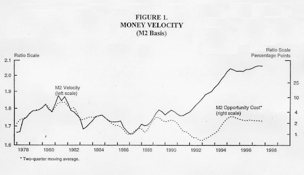
An Unconditional Rule: CROG The logic of the Friedman constant rate of growth (CROG) standard is that if the trend growth of real output is on the order of three percent per year, the trend growth of money of about four percent per year would permit for some low, and perhaps irreducible, inflation and also account for positive or negative trend changes in velocity. Were there expansionary or contractionary fiscal shocks, interest rates would rise or fall to stabilize output. As contrasted with the gold standard, overall liquidity would rise at a steady pace set to accommodate the normal growth in the economy, rather than an erratic pace set by worldwide gold discoveries. At the same time, CROG too contains potential difficulties. A first, pointed out by William Poole (1970),2 is that there could be shocks in the demand for money, related to technological or regulatory changes in the money creation system, foreign flows, or whatever. The CROG system would be buffeted by these, much as the gold standard system was buffeted by disturbances from the gold market. Moreover, as with the gold standard, there is no role in CROG for short term discretionary monetary actions. Even with automatic monetary stabilizers, economic cycles, under either the gold standard or CROG, could be long cycles and there would be no way to shorten them. This last issue brings up a key point of issue between those who became known as stabilization policy passivists, such as Friedman, and stabilization policy activists, such as Samuelson and Arthur Okun. To the passivists it is a virtue that there is no role for discretionary policy actions -- they feel that activist policy is intrinsicially either too little or too late (or too much or too soon) -- and they are perfectly comfortable in forswearing its use. Activists, on the other hand, might admit that certain historical policy mistakes had been made but still hold out the hope that discretionary actions could on balance stabilize the system. Pragmatically, the ability of a policy strategy such as CROG to stabilize the economy depends on the stability of money velocity. If velocity is stable, either constant (as the classical economists used to think) or slowly changing, keeping money growth on a smooth trend will keep overall GDP growth on a smooth trend. If on the other hand, velocity is not stable, by definition CROG would imply big cycles in total output unrelated to money growth. Figure 1 shows the actual path of velocity (M2 basis) over the 1959-97 period. There are clear upswings and downswings. Until 1990 these swings could be related to a measure of the opportunity cost of money (which still would not save a simple version of CROG), but since 1990 the movements in velocity cannot even be explained by movements in the opportunity cost of holding money. These swings now make it very difficult to use of CROG as a rule of thumb for monetary policy.
A Target Rule: Inflation Targeting While inflation targeting would seem to force central banks to become very specific about their policies, in fact the actual inflation targeting strategies have been more flexible. They have usually required the central bank to target between one and three percent inflation. They have also been defined in terms of some version of the underlying rate of inflation - the overall inflation rate less food and energy prices, the impact of exchange rates, excise taxes, and perhaps other clearly exogenous prices. Moreover, the real world inflation targets that have been instituted usually give the central bank an out, if this quarter it wants to worry about exchange rates, output gaps, or other economic goals (Ben Bernanke and Frederic Mishkin, (1997)).3 While not as loose as rules of thumb, nor have inflation targets been entirely rigid. The advantages and disadvantages of inflation targeting are much as for those of the other policy rules. On the one hand, central bank policy becomes more transparent and more logically related to what most people would say should be the underlying goal of central bank policy. On the other hand, there is a great loss of central bank flexibility. All central bank objectives apart from stabilizing prices are relegated to the background. Moreover, in the event of adverse price shocks, which impart a negative correlation between price and output movements, inflation targeting may force the central bank into undesirable contractionary policies just when unemployment is rising, though the fact that the targets can be written in terms of underlying inflation mitigates this concern. There are also timing questions. Often inflation targets are adopted when countries' inflation rates are clearly too high. In this event, should central banks be required (asked) to stabilize inflation gradually or abruptly? If there are nonlinearities in the inflation process, output gaps would normally be less if the central bank were to try to reduce inflation more gradually. A close relative to inflation targeting is nominal income targeting, suggested by Robert Hall and Greg Mankiw (1994).4 The main difference between inflation targeting and nominal income targeting is in the shocks. If there are price shocks, nominal income will not change as much as inflation, and the central bank would be better off targeting nominal income than inflation directly. On the other hand, if there are output productivity shocks, these shocks could alter nominal income and force the central bank to expand or contract even if inflation were on target. In general it is difficult to tell whether price shocks or productivity shocks will be larger and more prevalent, and hence whether nominal income targeting will or will not improve on inflation targeting.
A Feedback Rule: Taylor's Rule Taylor works backwards by determining how the federal funds rate, a short term interest rate, should respond to inflation and output. Using the funds rate directly eliminates the influence of shocks in the demand for money. These now become details that only the trading desk has to worry about. But working out the response patterns preserves the desirable stabilizing properties of a CROG rule. The Taylor rule can be expressed in a simple formula
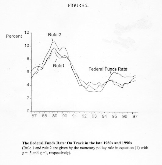
where PFR is the prescribed federal funds rate in nominal terms, the magnitude to be set by the monetary authorities. The equilibrium funds rate in real terms is r* and the actual rate of inflation is p. The deviation of output from its long-term trend is y and desired inflation is p*. While Taylor's rule is often expressed in terms of contemporaneous values of inflation and output, if there are lags in monetary policy, p and y could be forecast values, so that monetary policy could be made forward-looking. Suppose that monetary authorities were close to policy-making bliss, with no actual or forecast output or inflation deviations. Then the authorities would simply set the nominal funds rate at r* + p*, its desired long run value. If there were an inflationary shock, the monetary authorities would raise the funds rate by 1.5 times the change in inflation (the derivative of PFR with respect to p). This means that the real funds rate would rise as inflation rises, preserving the overall system stabilizing properties. If on the other hand, there were a recession, either current or forecast, the implied negative value of y, or output gap, tells authorities to lower the funds rate. The coefficient levels of .5 were inferred by Taylor from the properties of large simulation models of the time, though later research has shown that larger response coefficients would make the rule even more stabilizing (Andrew Levin, Volker Wieland, and John Williams, 1998).6 The adjustment coefficients already build stabilizing properties into the Taylor rule. If inflation rises, the rule tells the Fed to raise the real federal funds rate. If output falls, the rule tells the Fed to lower the real funds rate. But there could be even more stability implicit in this rule than meets the eye, through the behavior of long term bond rates. For any given funds rate, if output rises the spread between long term interest rates and the funds rate will rise and dampen output demand. If output falls, the spread will fall and stimulate output demand. So there are direct stabilizing properties built into the rule, and indirect properties through the behavior of long term bond markets. While such a simple rule might seem woefully inadequate as a descriptor of complex, subtle monetary policy, it turns out to explain actual monetary behavior in recent years quite well. Figure 2, taken from Taylor's 1998 paper, shows the plot of the actual funds rate over the 1987-1997 period. Rule 1 uses the coefficients of .5 and .5; rule 2 doubles the output response coefficient (g in the Figure). By historical standards, the 1987-97 decade was a good decade for the Federal Reserve, with only one recession and with gradually declining inflation rates. The equation tracks the actual path of the federal funds rate over this era of relatively successful policy very well. One could make the fit even closer by fitting equation 1) econometrically -- the fit becomes tighter and the estimated response coefficients rise. While most actual voting members of the open market committee during these years would probably be horrified that their behavior could be captured in such a simple equation, it seems that it can be.
Taylor (1998) himself takes the reasoning further by going farther back in time, to eras when central bank policy was less successful. He uses his rule to show that:
Many fans of Taylor's rule are reluctant to take the analysis this far. First, there is a technical question -- Athanasios Orphanides (1997)7 shows that Taylor's clear results become much more muddled when the actual data that were available to policy-makers at the time are inserted into the rule. Moreover, the Taylor rule presumes that monetary policy is independent in the sense that the Fed is free to vary the funds rate. Since the United States was on fixed exchange rates in the early 1960s, monetary authorities would have been substantially less free to lower the funds rate, as Taylor's rule would have recommended. Finally, there is a question of historical context. If the Federal Reserve were confronting the overhang of fifteen years of accelerating inflation combined with very large anticipated budget deficits, as it was in the early 1980s, policy might be forgiven a modest overadjustment according to the Taylor rule. But while there are problems with Taylor's historical analysis, the central conclusion of this analysis -- that monetary policy was far too easy most of the time (1965-79) and could have benefitted from a rule is certainly borne out by others (see Richard Clarida, Jordi Gali, and Mark Gertler (1998)).8 Taylor's cautious implication is that sometime in the 1980s, well before Taylor wrote his path-breaking paper, monetary policy has gotten on track and has pretty much stayed on track since. After all these years the Fed may finally be learning how to conduct monetary policy.
Uncertainties Perhaps. But there are uncertainties all over the place, both about the Taylor rule and indeed about rules in general. At the present time there are at least four main uncertainties about the Taylor rule. The inflation objective. The Taylor rule requires the monetary authority to get specific about price stability. Exactly what index is the Fed trying to stabilize, at exactly what level? Because there are well-known measurement problems with all price indeces, it is not necessary for the Fed to shoot for zero inflation, but the Fed does have to shoot for p*, and it certainly has to know whether actual or forecast inflation is above or below p*. That is not so hard when the economy is clearly suffering from inflation by anybody's definition, but it can become tricky as inflation declines and approaches its goal. The output objective. Uncertainties are even worse as regards the output term. Deviations of output from its trend are usually defined in terms of the so-called non-accelerating inflation rate of unemployment (NAIRU). If, for example, the actual unemployment rate is above NAIRU, there is an implied output gap and the Taylor rule tells the Fed to lower the funds rate. As with the inflation term, the Fed must then know where NAIRU is, and know whether current or forecast unemployment implies a positive or negative output gap. The unexpectedly quiescent behavior of inflation in the face of low unemployment in the late 1990s has led economists into major soul-searching about NAIRU. Whereas earlier in the decade most economists would have pegged NAIRU at about six percent, now opinions and estimates range all over the map. A recent Journal of Economic Perspectives (1997)9 symposium finds some economists who still believe in a stable NAIRU, some who believe in the concept of NAIRU but argue that its level changes, and some who think the whole concept is a snare and delusion. While the notion of a time varying NAIRU is conceptually attractive, there is again a question about how much time varying NAIRU should do, with respect to what. This NAIRU uncertainty then transfers over to output gap uncertainty. For the Fed to lean against the wind of output gaps, it has to know what the output gaps are, and that too can become quite tricky as unemployment approaches its desired level. The equilibrium funds rate. Even if inflation and output are on target, the Fed still has to determine what value to use for r*, the equilibrium real federal funds rate. An easy approach is to get that by the regression method - simply fit the Taylor rule and compute r* from the regression intercept. The problem with this approach is that it is only descriptive - fitting the Taylor rule only estimates how previous policy-makers might have responded to inflation and unemployment. To get to the normative concept of what the equilibrium real funds rate should be is harder. One approach might be to use the rate on newly-introduced long term indexed bonds as a measure of the equilibrium real interest rate for an economy that saves roughly as much as that of the United States. The saving clause is necessary because in most economies long-term equilibrium real interest rates depend on national saving rates. Subtracting a stable price term structure premium then gives an estimate of r*. There might be other ways of inferring r*, but however that is done, it must be done. Lags. A last problem in applying the Taylor rule is lags. Since there are long (and perhaps variable) lags in the impact of monetary policy, monetary policy must in principle move well in advance of the inflation and output gaps. These gaps then have to be forecast, and the forecast in principle must be for a period far enough ahead that monetary policy can act in a timely matter. This is a strong requirement and one can get misleading policy prescriptions by not looking ahead far enough, as is shown by David Small (1996).10 So the Taylor rule generally describes monetary policy well in years when policy was relatively successful, and also generally describes how monetary policy may have gotten off track in years when policy was less successful. It has desirable theoretical and stabilization properties. It gives clear signals when output and inflation are far from their target values. Yet it can still be very difficult to apply such a rule. There are interpretation problems on all the relevant targets - desired inflation, desired output, and the desired equilibrium funds rate. The rule may also have to be applied well in advance to be successful. The rule gives guidance, but certainly not complete guidance.
Implications The uncertainties implicit in using any rule of thumb, however well it might have performed in the past, are probably sufficient that policy-makers should retain their discretion. There can also be periods when the Fed is pursuing multiple goals. At the same time, the science of rule-building may have advanced to the point where monetary rules of thumb might play some useful role in the conduct of monetary policy. Myriad short term uncertainties and special factors mean that rules still cannot deal with many ad hoc situations. But in view of the deeper uncertainties about how hard monetary authorities should lean against what wind, rules of thumb might give good guidance to policy-makers. They might help authorities avoid large and persistent mistakes. Rather than replacing judgment, in the end rules may aid judgment. |
|
Footnotes Note. I have benefitted from the comments of Joseph Coyne, Roger Ferguson, Robert Frank, Donald Kohn, David Lindsey, Laurence Meyer, Athanasios Orphanides, Susan Phillips, Alice Rivlin, David Small, and Volker Wieland. 1 John Taylor, "A Historical Analysis of Monetary Policy Rules" (Stanford University, 1998). 2 William Poole, "Optimal Choice of Monetary Policy Instruments in a Simple Stochastic Macro Model," Quarterly Journal of Economics, vol. 84 (May 1970), pp. 197-216. 3 Ben S. Bernanke and Frederic S. Mishkin, "Inflation Targeting: A New Framework for Monetary Policy?" Journal of Economic Perspectives, vol. 11 (Spring 1997), pp. 97-116. 4 Robert E. Hall and N. Gregory Mankiw, "Nominal Income Targeting," in N. Gregory Mankiw, ed., Monetary Policy (University of Chicago Press, 1994), pp. 71-94. 5 John Taylor, "Discretion Versus Policy Rules in Practice," Carnegie-Rochester Conference Series on Public Policy, vol. 39 (December 1993), pp. 195-214. 6 Andrew Levin, Volker Wieland, and John C. Williams, "Robustness of Simple Monetary Policy Rules Under Model Uncertainty" (Board of Governors of the Federal Reserve System, 1997). 7 Athanasios Orphanides, "Monetary Policy Rules Based on Real-Time Data" (Board of Governors of the Federal Reserve System, 1997). 8 Richard Clarida, Jordi Gali, and Mark Gertler, "Monetary Policy Rules and Macroeconomic Stability: Evidence and Some Theory" (New York University, 1998). 9 "The Natural Rate of Unemployment," Symposium, in Journal of Economic Perspectives, vol. 11 (Winter 1997), pp. 3-108. 10 David Small, "The Simple Analytics of Choosing the Optimal Response Parameters in a Monetary Policy Rule for Nominal Income Targeting" (Board of Governors of the Federal Reserve System, 1996). |
|
|