PAPER OR PLASTIC? THE EFFECT OF TIME ON CHECK AND DEBIT CARD USE AT GROCERY STORES1
Keywords: Payment systems, consumer behavior, checks, debit cards
Abstract: Money evolved because barter is too time consuming. In barter, buyers and sellers exchange goods for goods. Exchanging goods for goods means that buyers have to search for sellers with whom they have a "double coincidence of wants".2 This search is potentially very time consuming. In monetary systems, buyers and sellers exchange money for goods. The search for trading partners is eliminated, and thus money reduces a potentially time consuming activity. This implies that money saves time for transactions. In this way, there is an intrinsic connection between money as a medium of exchange and time for transactions. Given the intrinsic connection between money as a medium of exchange and time for transactions, one begins to wonder whether time influences the type of medium of exchange used. Media of exchange depend on the technology and the economy of the day. Ancient Greece used gold coins as a media of exchange, while other societies used cattle, grain, or paper. Changes in the use of media of exchange can be linked to their relative efficiencies as media of exchange. For example, the introduction of paper notes to replace silver coins in Scotland led Adam Smith to comment that "the substitution of paper in the room of gold and silver money, replaces a very expensive instrument of commerce with one much less costly, and sometimes equally convenient."3 Today, there are four media of exchange commonly available to U.S. consumers: cash, check, credit card and debit card. These are relatively different physical media. Cash and check are pieces of paper, credit cards and debit cards are pieces of plastic. While the exact amount of cash use is unknown, consumer use of credit cards, debit cards and checks have changed in the past decade. From the mid 1990s to today, debit card use and holdings increased substantially, while check use declined.4 This paper offers evidence that one factor contributing to this change may be the time it takes to conduct a transaction. Economists have long recognized that costs of media of exchange can be significant and potentially affect the media of exchange used (Baumol [1952], Tobin [1956], Whitesell [1992], Santomero [1974], Santomero and Seater [1996]). In particular, shopping-time models and general equilibrium models of the transactions demand for money determine equilibria by examining the time costs for transacting with competing media of exchange. Minimizing these time costs is a central objective of the sellers and buyers in these models. Indeed, models of media of exchange including Karni [1973], Dowd [1990], and Shy and Tarkka [2002] predict that these expected time costs of exchange are potentially important when explaining equilibria. Moreover, recent payment innovations such as transponder devices used to pay for tolls, food and gas appeal to retailers by minimizing time costs for checkout. Buyers are similarly wooed by the convenience and time savings that these products offer.5 Finally, experience tells us that different media of exchange take different lengths of time to use. It takes longer to write a check for twenty dollars than it does to hand over a twenty dollar bill. Although there is theoretical research and anecdotal evidence that suggest time is an important element in determining the use of media of exchange, there is little empirical work documenting the magnitude of this effect. Perhaps this is due to a perceived lack of data (Hancock and Humphrey [1998]). Most of the data used previously to study payment behavior are based on surveys, either of sellers (ten Raa and Shestaloval [2002] or buyers (Avery et. al [1987], Boeschoten [1992], Kennickell and Kwast [1997], Stavins [2001], Mester [2003], Hayashi and Klee [2003]). These surveys find that time costs for transactions significantly affect both use of media of exchange and overhead costs for transactions. The weakness of these studies is that none examines seller and buyer behavior contemporaneously. Because the length of time of a transaction depends on seller and buyer behavior, no one survey can tell the whole story. To overcome weaknesses from survey data, this paper uses scanner data from grocery store transactions to examine time costs associated with media of exchange. Grocery store scanner data has been used extensively in other contexts, for example, in estimating elasticities of demand for consumer products (Chevalier, Rossi and Kashyap [2003]) and in constructing price indexes for goods (Feenstra and Shapiro [2003]). Scanner data is an ideal medium for examining time costs associated with media of exchange as well. First, these data represent actual market exchanges, are very accurate, and are available at a very high frequency. Second, grocery store retailers spend much time and effort in minimizing the length of time for checkout transactions, partly driven by the industry's relatively low margins - the average after-tax net profit as a percent of total sales was approximately 1 percent in fiscal year 2003.6 And third, everyone eats, everyone eats often, and everyone shops for groceries. Because groceries are perishable, consumers shop often, and thus this type of exchange is arguably one of the more frequent that a typical consumer makes. In fact, food purchases from grocery stores and other retail outlets represented 6.2 percent of disposable personal income in 2001.7 The scanner data used in this analysis are unremarkable and similar to that used in other scanner data studies. They contain the data items found on a typical grocery store register receipt. Each transaction has a time stamp, as well as information on the number of items bought, the value of the sale, the number of store and manufacturer coupons, and the payment type used. These items represent many of the observable factors that potentially affect both seller and buyer in determining the length of time of a transaction and payment choices. But unobservable factors also are likely to affect payment choices and the length of time of the transaction. Availability and the effect on the consumer's overall financial portfolio necessarily affects consumer's choices of payment instrument. While there are six different payment types commonly used to purchase groceries - cash; check; credit card; debit card; Women, Infants and Children (WIC); and food stamps - there is no information on the payment types that the particular consumer had available.8 Moreover, information detailing credit availability or checking account balances for consumers is unavailable in the data. Another factor that potentially affects buyers' choice of payment instrument is the consumer's expectation of the length of time of the transaction with the payment instrument, relative to other payment instruments. While the actual length of time of the transaction is observed, expectations are unobservable. Moreover, there is no information on how long the transaction would have taken if the buyer chose a different payment instrument. In order to control for availability and financial portfolio factors, the analysis uses debit card and check transactions only. Checks and debit cards both transfer funds from checking accounts; thus there should be little difference in availability or impact on consumers' financial portfolio, conditional on having the account, and the analysis is focused specifically on the effect of time on the choice of media of exchange. Furthermore, in order to control for the unobserved expectation of the length of time of a transaction, the analysis constructs expected transaction times following the method outlined by Lee [1978, 1979, 1981] and used in later work by Brueckner and Follain [1988], Dowd, Feldman, Cassou and Finch [1991] and Oettinger [1999]. Within this structure, the results indicate that consumers choose debit cards over checks in part because they expect debit card transactions to be faster than check transactions. Controlling for the number of items bought, the number of coupons used and the day of the week, check transactions are, on average, predicted to be approximately 40 seconds longer than debit card transactions. Using this predicted difference, the probability of using a debit card increases as the predicted percentage time difference between checks and debit cards increases. Interestingly, the results suggest that debit card users are, on an absolute basis, more time sensitive than check users, and thus the absolute predicted difference is negatively correlated. Time factors significantly determine use of media of exchange, and sensitivity to these time factors depend on the income, age and demographic characteristics of the local market. The results are robust to two models of consumer behavior. In the first model, consumers make a choice instantaneously at the point of sale. They form an expectation of the length of the transaction given the items they bought and the value of the sale. Consumers then choose the payment instrument that minimizes the time for that particular transaction. Another model consistent with the results posits that consumers choose to use a check or debit card based on their expectation for the distribution of transactions they make and their preferences in terms of time spent at the checkout line. Given this distribution, consumers make a choice between a check and a debit card (at home, say) and carry only that payment instrument to the store. Both interpretations are consistent with the empirical result that time factors significantly affect the choice of media of exchange.9 Importantly, there are a few caveats with these results. The first caveat is that the analysis implicitly assumes that all debit card users could use checks, all check users could use debit cards, and that the costs associated with each are the same. This may not be the case. Consumers who have a strong preference for minimizing the length of a transaction would actively seek out a checking account that offers debit cards services. In contrast, those who have a strong preference for checks do not seek such accounts. In both cases, while the fees may differ according to payment type, the opportunity cost associated with the account should still be identical. In this interpretation, the observed payment instrument use reflects consumer preferences accurately and indeed, could potentially strengthen the results. Second, consumers authorize debit card transactions in two different ways. Consumers can enter a PIN, or personal identification number, or consumers can sign. If a consumer enters a PIN, it is called a "PIN-based" debit card transaction, and is primarily routed over networks such as NYCE, STAR and PULSE, or the Visa and MasterCard PIN-based networks, Interlink and Maestro/Cirrus. If a consumer signs, it is called a "signature-based" debit card transaction, and is usually routed over the Visa and MasterCard credit card networks. There is no way to distinguish signature-based debit card transactions from credit card transactions in these data. Thus, the debit card results presented here are PIN debit card transactions only. Despite the fact that the analysis necessarily uses only a subset of all debit card transactions, there is one advantage to using only PIN debit card transactions. In general, consumers may obtain cash back at the point of sale with a PIN debit card transaction, but cannot obtain cash back with a signature-based debit card transaction. In addition, consumers may obtain cash back at the point of sale using a check. In this way, PIN debit card transactions and checks are closer substitutes than signature debit cards and checks. This helps to isolate further the effect of transaction time on payment choice. The paper is organized as follows. Section II gives an overview of the problem, sets up the model, and discusses the econometric issues. Section III describes the data used. Section IV provides the results of estimating the model, and section V concludes. In order to give perspective for the analysis, figure 1 plots the distribution of the time of transactions by tender type. The time for the transaction is the "ring time," which is calculated as the number of seconds between the first item crossing the scanner to the close of the cashier's drawer - the amount of time the cashier spends ringing up the transaction. The data contain no information on how long the customer spent waiting in line before the transaction occurred, whether it was two seconds or ten minutes. The These functions show that there is a relatively higher density of cash transactions with shorter ring times, and a relatively higher density of check transaction with longer ring times. Card products, debit cards and credit cards, take similar lengths of time, but their estimated densities are slightly different. These densities are reflected in the aggregate statistics. Cash transactions have the lowest mean ring time, at approximately 56 seconds, while checks have the highest mean ring time, at approximately 148 seconds. Credit card and debit card transactions have similar mean ring times, at 112 and 101 seconds, respectively. Experience tells us that transactions with 5 items usually take a shorter length of time than transactions with 20 items. Figure 2 shows this clearly. The The final step is to investigate more closely the distribution of times for check and debit card transactions, the focal point of the analysis in this paper. One unique feature of check and debit card transactions is that consumers can obtain "cash back" with a transaction. This feature potentially affects both the length of time of a transaction and payment choice. Figure 3 plots only check and debit card transactions, and divides these transactions by whether or not the customer obtained cash back with a transaction. The Although it may seem that these times are small in magnitude, they add up to much more than small change. From the retailer's point of view, the sum of the individual transaction times is a significant share of the total time the retailer spends on payment processing.11 From the customer's point of view, the time differentials can be expressed in terms of the opportunity cost according to the individual's wage rate. Depending on the wage, the shadow value of payment time can range quite substantially, and possibly could add up to dollars in lost time over the month. These incentives for both the retailer and the customer to minimize the time for the transaction form the backbone of the analysis. Figures 1, 2 and 3 show that there is a potential relationship between transaction time and media of exchange. In order to investigate this further, the analysis that follows models the exchange between buyer and seller as a two-stage endogenous switching regression model. In particular, the model tests whether consumers' choice of payment instrument depends on the expected length of the transaction. The model and econometric methodology follows Lee [1978], who analyzed the effect of expected wage differentials on union participation choices. Subsequent work used this type of analysis to examine choices of mortgages, health care plans, and stadium vendor labor supply. Following Lee [1978], the framework is: Equation (1) can be interpreted as the cashier's instantaneous cost minimization function. The cashier is assumed to react to each transaction differently, and minimize time costs according to the characteristics of the transaction. These factors are represented by Equation (2) is the consumer's choice problem. The vector As discussed above, there are two potential econometric difficulties with this specification. The first problem occurs in equation (2). If the econometrician observes all factors that could potentially affect payment choice but for an independently and identically distributed error term, one can form the probability of using a particular payment instrument based on an assumption regarding the distribution of this error term. McFadden [1973] showed that if this error term follows an extreme value distribution, the resulting probabilities and specification are consistent with utility maximization. But, as the data contain no personally identifiable information, it is unlikely that the econometrician observes all factors that could potentially contribute to payment choice. For example, there is no information on the availability of media of exchange, or information on opportunity costs associated with accounts. Assuming that all of these factors could be explained by an independently and identically distributed error term may be incorrect. In particular, these missing factors could be correlated with the variables in In order to isolate the effect of some of these factors, using a specification similar to that in Goolsbee and Petrin [2004], the unobserved factor The second potential econometric difficulty involves the length of time for the transactions. While the length of time for the transaction with the payment instrument actually chosen is observed, the expected length of time for the transaction with any other payment instrument is not. As a result, the differences
As explained above, the econometric specification is similar to a two-stage switching model with endogenous regressors.13 The estimation procedure is in three parts. The first step is to estimate a reduced form probit specification. In particular, equation (2) is rewritten as The covariance matrix of the error terms
Including these terms allows equation (1) to be rewritten as The consistent estimates
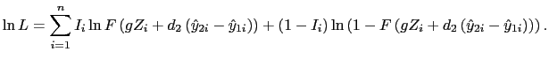
The final step is to re-estimate the probit equation, including the predicted transaction length times. The parameter estimates obtained maximize the log-likelihood function, There are two main data sources used in the analysis: scanner data and U.S. Census Bureau census tract data. The scanner dataset is proprietary and is from a regional grocery store chain, defined as a firm with between 11 and 150 stores. According to one classification, local independents have between 1-10 stores, regional firms have from 11 and 150 stores, and large retailers have more than 151 stores.15 Importantly, all stores in the chain accept cash, checks, credit cards, and debit cards for payment. In addition, all stores accept WIC and food stamps. Different stores have different services, for example some retail outlets have a floral department or an attached pharmacy. The scanner data are over 10 million checkout transactions over a three month period, from September to November, 2001. For computational tractability, the estimates are based on a sample. The sampling procedure is as follows. From the population of over 10 million transactions, a random sample of 100,000 observations was drawn without replacement. This process was repeated 100 times, to provide 100 samples. Thus, each subsample represents a sample without replacement, but observations may be repeated across subsamples. Most reported estimates reflect the results from evaluating the model on one random sample only. In general, results are qualitatively similar across random samples. However, some coefficients change sign and significance. These cases are noted within the text. The unit of observation is a checkout transaction, which represents one customer's total purchase at the point of sale. As the data are all from one retail chain with between 11-150 locations, each transaction has exactly the same information. The data contain the information commonly found on most register receipts from a purchase at the grocery store. These include the store number, the date of the transaction, the "ring time", the payment type, the amount of change received, and the number of coupons (both store coupons and manufacturer coupons). Importantly, all data were stripped of personally identifiable information. These information items include, but are not limited to, credit card and debit card numbers, loyalty card numbers, WIC and food stamp identification numbers, and check identification numbers. The data also do not include any way to match item codes to actual items, but there is information on the general department code for the item (for example, meat, general grocery, or produce). The second data source used in the analysis is 2000 census tract information from the U.S. Census. The addresses of the retail outlets were matched with census tract level information from the U.S. Census Bureau to proxy for demographics of the local market. Evidence suggests that people shop locally for groceries.16 Thus, census tract information may proxy for heterogeneity that may exist in length of time of transactions due to demographics of the local market. These census tract variables were matched with transactions by the retail outlet number on the scanner dataset. Scanner data have a number of unique advantages compared with survey data that contain information on payments. First, these data represent actual buyer and seller behavior, and thus eliminates measurement and sampling error associated with surveys. Second, the quantity of data allows for precise parameter estimates and estimation of effects that may not be able to be determined from a survey dataset. Third, these data represent the entire exchange, while most survey datasets focus on only the buyer or the seller. Using scanner data does, however, have some limitations. First, the sheer quantity of data can be computationally burdensome. Second, as noted in the introduction, there is no way to distinguish PIN debit card transactions from signature-debit card transactions. Finally, as noted above, there is no personally identifiable information contained in these data. The census tract information is the best proxy for demographic information that has been shown to be a key determinant of payment choice for consumers in previous research. Table 1 gives definitions and table 2 gives summary statistics for the variables used in the estimation procedure. Approximately 56 percent of the sample are check transactions; 44 percent are debit card transactions. The median ring time for any transaction is 109 seconds, or one minute and 49 seconds. The mean ring time is 128 seconds, which shows that there are some very long outlier transactions. The maximum ring time was top-coded at ten minutes, or 600 seconds, but the longest ring time in this random sample is 597 seconds.17 The median number of items bought is approximately 12, while the mean number of items bought is 16.66. The median value of a sale is $28.81, and the mean value of a sale is $40.27. Most transactions do not use manufacturer coupons; the mean number of manufacturer coupons is 0.32. Overall, 17 percent of check and debit card transactions have cash back. Although the percentages do not differ greatly by tender type, the amount of cash back does differ substantially. Approximately 17.5 percent of debit card transactions have cash back, while 15.4 percent of check transactions have cash back. But, the average value of cash back with a check is about $50, while the average value of cash back with a debit card is approximately $25. Indeed, there may be limits on the amount of cash back that affects these levels. As outlined above, the estimation procedure is in three steps. The first step is to estimate the reduced form probit and construct the terms that control for selection bias in the time equation (1). The second step is to estimate the coefficients of the time equation (1). The third step is to predict values from the time equation and use these predicted values as independent variables in the structural estimation of equation (2). By design, the independent variables used in the second stage do not overlap with the independent variables used in the third stage, in order to minimize effects of using imputed regressors on the standard errors. Physical characteristics of the sale - the number of items bought, the number of manufacturer coupons used, the day of the week - are included in the second stage, while monetary characteristics of the sale - the value of the sale, the number of store coupons (interpreted as the number of items bought that were on sale) and the demographics of the local market are not included. Intuitively the breakdown makes sense. Previous research indicates that demographics significantly affect payment choice by consumers. The reasonable assumption on the cashier side is that the cashier treats all customers the same in terms of speed of transaction, regardless of age, education or gender. The only instance in which the physical versus value logic was not followed is with the total value of cash back and the cash back indicator. The value of cash back was included in the time regression and an indicator was included in the structural probit estimation. Although this distinction may be viewed as arbitrary, it was made for three reasons. First, the estimated coefficient on this variable can be interpreted as the cost per dollar in terms of time of getting cash back at the point of sale. The indicator equals one if the transaction had "cash back", which is calculated as the change from these transactions. Second, the desire to get cash back at all will influence whether a customer uses a PIN debit card or a check over using cash or a credit card. This indicator allows the econometrician to control for this effect. And third, the length of time of the transaction may be affected to a greater extent by the amount of cash back - it takes longer to count out fifty dollars than it does to hand over a twenty dollar bill. The first stage results for the reduced form probit are not reported. The second stage results for the ring time regressions are shown in tables 3(a), (b) and (c). In table 3(a), the dependent variable is the transaction time in seconds; in table 3(b), it is the natural logarithm of the transaction time. In both of these tables, all independent variables are not transformed. In table 3(c), the dependent variable is the natural logarithm of the transaction time and the independent variables are also in logarithms, except for the correction terms. In addition, two sets of standard errors are reported for all estimation results. The first set is the corrected standard errors, using the method in the Appendix. The second set is the uncorrected OLS standard errors. As is apparent from the table, the uncorrected standard errors are not too different from the corrected standard errors.18 Turning first to the ring time results, in both the debit card and check results, the number of items bought, the number of manufacturer coupons used, and the dollar amount of cash back significantly affect the transaction time. The intercept for each equation is very different in magnitude - approximately 77 for the check estimates and approximately 40 for the debit card estimates. Thus, if all other covariates were set equal to zero, check transactions would take approximately 37 seconds longer, or almost twice as long. Interestingly, the magnitudes of the other coefficients are similar in both specifications. The positive sign on the items bought coefficient appears in both the check and the debit card equations, which implies that increases in the number of items bought increases transaction time. The negative sign of the items bought squared coefficient shows that the rate of increase decreases with items bought and gives evidence of a concave time function. Positive signs on the number of manufacturer coupons coefficients indicate that transaction time increases with the number of manufacturer coupons, which agrees with intuition concerning the time both the cashier and the customer use to handle the coupon. The day effects are normalized to Sunday, Day 1. Significant and positive signs on the Day 6 coefficient appear in all the time equations estimates, so that the observed length of time of transactions is statistically significantly longer on Friday than on Sunday for both check and debit card transactions. Significant and positive signs appear in the check equation estimates for Wednesday and Thursday as well. In general, all other day coefficients are not significantly different from zero, which implies that they are not significantly different from Sunday. The positive sign on the value of cash back can be interpreted as the per-dollar cost of getting cash back at the point of sale. The coefficients in both equations are positive and significant, and similar in magnitude. The coefficient in the check equation is greater than the coefficient in the debit card equation. This suggests that the absolute per-dollar cost in terms of time of obtaining cash back with a check is higher than the absolute per-dollar cost of obtaining cash back with a debit card, measured in terms of time. Dollar per dollar, it's absolutely more expensive in terms of time to get cash back with a check than with a debit card. The selection terms in the last row of each of the tables indicate that there is a negative truncation effect for debit card use and no significant truncation effect for check use. This implies that debit card users may be more time sensitive, as an unobserved factor that predicts debit card use is correlated with an unobserved factor that determines the length of time of the transaction. In plain English, debit card users may be speedier than other shoppers. For example, they may put all of their items on the belt before the cashier starts ringing up the transaction, they may pay faster, or they may chat less with the cashier in order to get out of the store faster. They also prefer debit cards because debit cards are faster than checks. In less plain English, there may be an unobserved factor that affects the probability of using a debit card that is also correlated with an unobserved factor associated with faster transactions. Thus, the data exhibit sample selection bias for debit card transactions. In contrast, there is no such selection for check use. However, the insignificance of the selection coefficient in the check equation does not indicate that individuals who use checks are purposely slow. The Table 3(b) reports the results from estimating the model using the natural logarithm of the transaction time as the dependent variable. In general, the results reported here are consistent with the results reported in table 3(a): the number of items bought, the number of items bought squared, and the amount of cash back have significant coefficients in both the debit card estimation results and the check estimation results. The day results are also similar, except the coefficient on the day 7 variable, Saturday, is significant in the check specification. Interestingly, the magnitude of the coefficient on the cash back variable is higher in the debit card equation than in the check equation. This result suggests that the percentage per-dollar cost of obtaining cash back with a debit card is higher than the percentage per-dollar cost of obtaining cash back with a check, measured in terms of time. Dollar per dollar, it's relatively more expensive to get cash back with a debit card than with a check. As in table 3(a), the coefficients on the selection terms in table 3(b) show negative selection for debit card transactions and no significant selection for check transactions. The sign on the selection term for the check transactions should not be interpreted as evidence for truncation one way or the other, as the sign changes across different random samples. Debit card users still exhibit relative speediness for transactions. The Table 3(c) reports the results from estimating the model using the natural logarithm of the ring time, but changing the specification to include the natural logarithm of the number of items bought.19 The results are consistent with those in tables 3(a) and 3(b) for the number of items bought. Indeed, the coefficients are almost exactly the same in both the debit card and check equations for this specification. The magnitude of the manufacturer coupon coefficient is greater in the debit card equation than in the check equation. For the days of the week, Friday is significant in both equations, while Thursday and Saturday are significant in the check equation as well. The coefficients on the cash back terms can be interpreted as the semi-elasticity of the ring time with respect to the amount of cash back. As is evident from the table, the magnitude of this elasticity is greater for debit card transactions than for check transactions, almost by a factor of two. Thus the percentage increase in the length of time of a transaction per dollar of cash back is greater for debit card transactions than for check transactions. Dollar per dollar, the time increase for debit cards is greater than the time increase for checks. These results point to high fixed time costs of using checks, with a relatively lower variable cost per dollar in terms of time, and a low fixed time cost of using a debit card, with a relatively higher variable cost per dollar in terms of time. Consistent with the results in tables 3(a) and 3(b), the results in table 3(c) show there is a negative truncation for debit card transactions and no significant truncation for check transactions. In this case, however, the sign could potentially be interpreted as showing a possible positive truncation for check transactions. The luxury of these data is the ability to compare estimates across random samples of a population. While the results reported here reflect one random sample, inspection of other random samples show significant positive truncation for check transactions.20 In plain English, check writers may be slower than other shoppers. In less plain English, there may be an unobserved factor that affects the probability of using a check that is also correlated with an unobserved factor associated with slower transactions. Thus, the data may exhibit sample selection bias for check transactions. As explained above, the estimation results from the second stage are used to predict how long each transaction will take with a check and with a debit card. From these predictions, time differentials for each transaction are calculated. These time differentials are then used in the structural probit estimation. The time predictions and differentials, however, are interesting in their own right, and this section explores their properties. Tables 4(a) and 4(b) detail the results. The analysis uses three types of predicted time calculations. The first uses the results in table 3(a), and calculates predicted times as
As shown in table 4(a), the average predicted length of time of a transaction with a check is 139 seconds, and the average predicted length of time of a transaction with a debit card is 101 seconds. The median of the predicted check times is 122 seconds, and the median of the predicted debit card times is 84 seconds, which shows that the distribution is skewed. Using the formula in (10), the average of the predicted time differentials is 39 seconds. More than 99 percent of transactions have a predicted length of time with a check that is longer than the predicted length of a transaction with a debit card. There are, however, a few exceptions. The lowest predicted time difference is approximately -81 seconds, implying that given the particular transaction's combination of number of items bought and number of coupons, it is predicted to be faster to write a check.21 In contrast, the highest predicted time difference is approximately 85 seconds faster to use a debit card.22 Inspection of these individual transactions shows that while these transactions are outliers with regards to the number of items bought and the number of coupons, they are plausible. Examining average percentage time differentials between check and debit card transactions is also instructive. These are calculated as Table 4(b) shows breakdowns of these predicted time calculations by different classes of the independent variables: the number of items bought, the number of manufacturer coupons and the value of cash back. The breakdown by the number of items bought shows that the average predicted time difference first rises, then falls with the number of items bought. The percentage savings with using a debit card transaction is on average 40 percent for transactions in the 20th percentile for the number of items, 30 percent for transactions between the 50th and 60th percentile for the number of items items, and 16 percent for transactions on average for transactions between the 90th and 100th percentile of items. The predicted logarithm difference exhibits a similar trend to the percentage savings, showing a steady decrease as the number of items increases. These results, coupled with the similar parameter estimates reported above, indicate that the time costs of checks are fixed costs, rather than variable with the number of items bought or the number of coupons used. Intuitively, this makes sense. A customer can write a check for a ten item transaction or a fifty item transaction; the amount of time to write the check is most likely similar. Moreover, if the number of items is large enough, it is likely that the consumer can complete most of the check information during the time the cashier runs the items across the sacanner. This may also contribute to a relatively higher incidence of check use in transactions with a greater number of items bought. The pattern for the time changes with respect to the number of manufacturer coupons is slightly different from the pattern with the number of items bought. The number of manufacturer coupons used shows a steady increase in the time differential for checks and debit cards as the number of coupons increases, rising from approximately 39 seconds for transactions without any manufacturer coupons, to approximately 43 seconds for the maximum number of coupons tendered. In percentage terms, this difference decreases from 31 percent to 20 percent, and the predicted logarithm difference decreases from 0.38 to 0.26. Again, this result points to a fixed cost of using a check versus using a debit card, which decreases in percentage terms as the overall length of the transaction increases. The cash back time pattern follows a different pattern than either the number of items bought or the number of manufacturer coupons. As the dollar amount of the cash back increases, the time differential between check and debit card transactions first dips slightly, then increases, going from 39 seconds, down to 38 seconds, and increasing to 41 seconds. The percentage time differential increases from approximately 30 percent to 33 percent, and then decreases to 31 percent. The difference in the predicted logarithm times increases from 0.37 to 0.40, and then decreases to 0.36. With the constructed predicted time differences above, the estimation procedure continues by estimating the full structural probit. The predicted time differences can be interpreted as the consumer's expectations of the time difference between using a check and using a debit card, and the analysis below examines whether this expectation is a significant factor in a consumer's decision to use a debit card. Tables 5(a), (b) and (c) report the results. Each table corresponds to a second stage specification. The dependent variable is a discrete zero or one;p one indicating that the customer used a debit card. Because this is a probit model, the coefficients are not easily interpretable in terms of percentages or effects on the probability of using a debit card. In order to aid interpretation, two marginal effects are reported. The first marginal effect is the mean of the derivatives across observations, calculated as The first specification results shown in table 5(a) uses the absolute differences calculated from the specification in table 3(a). The constructed time difference variable is the predicted time for a check transaction length minus the predicted time for a debit card transaction. The results show that the probability of using a debit card is negatively correlated with this differential. That is, as the difference in the length of time increases, the probability of using a debit card decreases. This result seems counterintuitive. However, this results is consistent with the possibility that an unobserved factor that affects the probability of debit card use is correlated with an unobserved factor that affects the length of time of transaction. For debit card transactions, these factors are negatively correlated; unobserved increases in the probability of using a debit card are correlated with unobserved decreases in the length of time of a transaction. When constructing the predicted lengths of time for the transactions, on average, the constructed predicted differentials between check and debit card transactions are shorter for debit card transactions than for check transactions. The predicted time differential is 38 seconds for debit card transactions and 39.5 seconds for check transactions. The results suggest that consumers who use debit cards may be more time sensitive on an absolute basis, and any differential in the length of time of a transaction will lead them to choose a debit card. The results in table 5(b) shows the estimation results from using the differences in the logarithm of the times for the transaction as an independent variable, corresponding to the parameter estimates in table 3(b). The differences in the predicted times based on a logarithmic specification can be roughly interpreted as a percentage difference in the length of time of the transaction with a check and with a debit card. The results show that an increase in the percentage differential between a check and a debit card transaction increases the probability of using a debit card. Transactions where the percentage differential is a greater percent of the total transaction time are more likely to occur with debit cards than with checks. The results in table 5(c) use the parameter estimates from table 3(c) to construct the time terms, and provides a robustness check for the specification in table 5(b). The results are similar to those in table 5(b), showing a significant effect of the percentage difference in the length of a transaction with a check and with a debit card on the probability of using a debit card. Although the primary focus of this paper is to investigate the relationship between time and payment choice, it is instructive to review the coefficients on the other factors that affect the probability of using a debit card as well. The probability of using a debit card decreases as the value of the sale increases, at an increasing rate. The elasticity calculations show that, on average a 10 percent increase in the value of the sale decreases the probability of using a debit card 2.4 percent in the first specification, 1.1 percent in the second specification and 4.7 percent in the third specification (tables 6 (a), (b) and (c) respectively). Thus, debit card use is relatively inelastic with changes in the value of the sale. However, this result is somewhat surprising, if one believes that all demand for money is based on the opportunity cost of funds. Both debit card and check transactions have the same affect on a consumer's overall financial portfolio. In theory, there should be no differential affect of the value of the sale on the choice between a debit card and a check. But, the results clearly indicate that this is not the case. This result points to characteristics of transactions other than the value of the sale that determine the demand for money, and represent an avenue for fruitful research. Continuing with the remaining transaction characteristics, the results show that an increase in the number of store coupons decreases the probability of using a debit card. Store coupons proxy for items bought on sale in this dataset. Thus, debit card users buy fewer items that are on sale than check users do, all other things equal. Again, the response is relatively inelastic, but the parameter is significant nonetheless. The final point to investigate are the effects of the demographics of the local market on debit card use. Interestingly, many of the demographic trends evident in estimates on family-level data appear at the aggregate tract level as well. A higher median tract income leads to a higher estimated probability of using a debit card. The age coefficients show that tracts with a larger proportion of relatively older householders are correlated with lower debit card use rates. In addition, tracts with higher levels of education are positively correlated with debit card use. High income, younger and more educated families are more likely to use debit cards than other families. These results at the tract level in general conform to these results. Table 6 provides some back-of-the-envelope calculations that provide support for the claims in the previous paragraph.24 Using data from the January 2001 National Compensation Survey and the predicted times for the 50th-60th percentile of items bought shown in table 4, the shadow values of payment choice can be easily calculated. The difference in price for checks and debit cards is 66 cents for the highest hourly earners, a substantial difference. Work by Bolt et. al (2005) shows that consumers indeed change payment choices when payment instruments are priced explicitly. The results in this paper show that consumers change their choices when faced with implicit costs as well. This paper offers new empirical evidence for old conclusions in monetary theory, namely, that transaction costs significantly affect the media of exchange used. The empirical results offer evidence that consumers choose debit cards over checks in order to minimize the amount of time it takes for a transaction. The estimation procedure controls for the endogeneity of the choice of a debit card or a check and the realized length of time it takes to conduct the transction. The results indicate that the expected percentage difference in the length of a transaction is a significant factor in consumer's choices of debit cards over checks. Holding all else equal, on average, check transactions take approximately forty seconds longer than debit card transactions. On average, debit cards take only 70 percent of the amount of time a check transaction takes. The higher the percentage time difference between debit card and check transactions, the more likely the consumer is to use a debit card. It is difficult to know to what extent the results presented here are affected by other factors that cannot be controlled for in the estimation procedure. For example, the design of the checkout line is likely to be endogenous to the payment types typically chosen at the point of sale. The retailer may choose to make PIN pads for debit cards easier for customers to use than the check writing platform. This would materially affect the estimation results. In order to control for these types of effects, a natural extension would be to extend the analysis to depend on a repeated interaction between consumer and retailer, and look at changes in use over time. In that case, consumer's expectations of time costs of payments could depend not only on their one-time choices, but also on expected future interactions with retailers. Similarly, retailers could look at transactions that were too costly in terms of time, and could refuse payment types or update their computer systems to avoid time costs. Many theoretical models of exchange incorporate intertemporal features. An interesting extension of the research presented here would be an empirical investigation of these types of effects. As explained in the text, each stage's standard errors should be corrected to account for the fact some terms are predicted from the previous stage. The standard errors reported in this paper reflect the necessary corrections. This section outlines the methods used, based on Lee [1982 There are two ring time regressions reported: one for the subsample that used a debit card and the other for the subsample that used a check. Using the OLS standard errors may lead to mistakes in inferences regarding parameters due to sample selection. This section outlines the method used to correct the standard errors, based on Lee [1978, 1979, 1982]. The notation follows Lee [1978], p. 422. The approximation to the correct asymptotic covariance matrix used is In this stage, the standard errors should be corrected to account for the fact that the
There are two log likelihood functions for the first stage, reflecting the two separate estimation procedures for
The log likelihood functions for the first stage are
Introduction
Overview, model, and econometric issues
Overview
![]() axis is the number of seconds in the transaction. The
axis is the number of seconds in the transaction. The ![]() axis is the kernel density estimate of the length of time of the transaction. This kernel density is calculated as
axis is the kernel density estimate of the length of time of the transaction. This kernel density is calculated as
![]() where
where
![]() and
and ![]() is the smoothing parameter
is the smoothing parameter![]() There is a separate density calculated for each tender type.
There is a separate density calculated for each tender type.![]() axis values are the number of items in a particular transaction. The domain represents the 50th to 75th percentiles of items bought in the data.10 The
axis values are the number of items in a particular transaction. The domain represents the 50th to 75th percentiles of items bought in the data.10 The ![]() axis values are the average ring time for that number of items in seconds. The lines represent each tender type. The average ring time increases as the number of items bought increases. As is evident from the graph, for each number of items bought, the average ring time is lowest for cash, and highest for checks. Interestingly, the space between these graphs stays relatively constant as the number of items bought increases, which gives some indication of a fixed effect of media of exchange on the length of time for a transaction.
axis values are the average ring time for that number of items in seconds. The lines represent each tender type. The average ring time increases as the number of items bought increases. As is evident from the graph, for each number of items bought, the average ring time is lowest for cash, and highest for checks. Interestingly, the space between these graphs stays relatively constant as the number of items bought increases, which gives some indication of a fixed effect of media of exchange on the length of time for a transaction.![]() axis is the number of seconds in the transaction. The
axis is the number of seconds in the transaction. The ![]() axis is the kernel density estimate of the length of time of the transaction. Separate densities are estimated for checks with cash back, checks without cash back, debit cards with cash back and debit cards without cash back transactions. Consistent with figure 1, the distributions for debit card transactions are centered around shorter ring times, while the distributions for check transactions are centered around longer ring times. Perhaps surprisingly, there is a relatively higher frequency of short debit card transactions with cash back, relative to debit card transactions without cash back. Indeed, summary statistics show that the average ring time for a debit card transaction with cash back is 96 seconds, while the average ring time for a debit card transaction without cash back is 102 seconds. Check transactions with and without cash back have similar average ring times, around 148 seconds.
axis is the kernel density estimate of the length of time of the transaction. Separate densities are estimated for checks with cash back, checks without cash back, debit cards with cash back and debit cards without cash back transactions. Consistent with figure 1, the distributions for debit card transactions are centered around shorter ring times, while the distributions for check transactions are centered around longer ring times. Perhaps surprisingly, there is a relatively higher frequency of short debit card transactions with cash back, relative to debit card transactions without cash back. Indeed, summary statistics show that the average ring time for a debit card transaction with cash back is 96 seconds, while the average ring time for a debit card transaction without cash back is 102 seconds. Check transactions with and without cash back have similar average ring times, around 148 seconds.The model and econometric issues
where ![]() is the length of time for transaction
is the length of time for transaction ![]() with payment instrument
with payment instrument ![]() and
and ![]() is the consumer's utility from the choice of payment instrument
is the consumer's utility from the choice of payment instrument ![]() .
. ![]() are observed variables that potentially affect the length of time of a transaction,
are observed variables that potentially affect the length of time of a transaction, ![]() is a vector of parameters to be estimated and
is a vector of parameters to be estimated and ![]() is an unobserved error term.
is an unobserved error term. ![]() are observed transaction characteristics that are constant across payment types,
are observed transaction characteristics that are constant across payment types, ![]() and
and ![]() are coefficients to be estimated, and
are coefficients to be estimated, and ![]() is an unobserved error term. The econometrician does not observe utility directly, but instead observes an indicator
is an unobserved error term. The econometrician does not observe utility directly, but instead observes an indicator ![]() which equals 1 if the utility of the transaction with payment instrument
which equals 1 if the utility of the transaction with payment instrument ![]() is greater than the utility of the transaction with all other payment instruments.
is greater than the utility of the transaction with all other payment instruments.
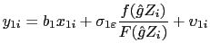
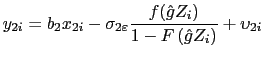
![]() . They include the number of items bought and the number of items bought squared,12 the number of manufacturer coupons, the day of the week, and the amount of cash the consumer receives back from the transaction. By assumption, cashiers do not adjust their behavior with a particular payment type nor steer customers to a faster payment type. Cashiers consistently act to minimize the length of time of the transaction and passively accept the payment type.
. They include the number of items bought and the number of items bought squared,12 the number of manufacturer coupons, the day of the week, and the amount of cash the consumer receives back from the transaction. By assumption, cashiers do not adjust their behavior with a particular payment type nor steer customers to a faster payment type. Cashiers consistently act to minimize the length of time of the transaction and passively accept the payment type.![]() includes factors that may affect consumer's utility of using a particular payment instrument, including the value of the sale, the value of the sale squared, the number of store coupons, and an indicator for cash back. In addition, the vector
includes factors that may affect consumer's utility of using a particular payment instrument, including the value of the sale, the value of the sale squared, the number of store coupons, and an indicator for cash back. In addition, the vector ![]() contains demographic characteristics of the local market. Previous research on family-level survey data consistently shows that consumer demographic characteristics significantly predict use and holdings of different payment instruments. The demographics included reflect these significant factors. The terms
contains demographic characteristics of the local market. Previous research on family-level survey data consistently shows that consumer demographic characteristics significantly predict use and holdings of different payment instruments. The demographics included reflect these significant factors. The terms
![]() are the expected difference in the length of time of the transaction with each payment instrument
are the expected difference in the length of time of the transaction with each payment instrument ![]() from the choice
from the choice ![]() . Statistically signficant coefficients
. Statistically signficant coefficients ![]() indicate that the expected difference in the length of time of the transaction is a significant predictor of payment choice
indicate that the expected difference in the length of time of the transaction is a significant predictor of payment choice ![]() .
.![]() , specifically, the demographics of the local market. Estimates of parameters that ignore these unobserved factors may be biased.
, specifically, the demographics of the local market. Estimates of parameters that ignore these unobserved factors may be biased.![]() can be written in two factors as
can be written in two factors as![]() .
.
![]() represents the account-based average of omitted attributes and other unobserved factors. Thus, by assumption,
represents the account-based average of omitted attributes and other unobserved factors. Thus, by assumption,
![]() is constant across payment choices that originate from the same transaction account and can be interpreted as an opportunity cost of using a particular payment instrument. In the context of a checking account, it is any interest or fees associated with the account as a whole that would apply both to debit card use and check use. Hence, debit card transactions and check transactions originating from the same checking account share the same
is constant across payment choices that originate from the same transaction account and can be interpreted as an opportunity cost of using a particular payment instrument. In the context of a checking account, it is any interest or fees associated with the account as a whole that would apply both to debit card use and check use. Hence, debit card transactions and check transactions originating from the same checking account share the same
![]() , and cash and credit card transactions have different
, and cash and credit card transactions have different
![]() from each other and from debit cards and checks. Estimating the model on the subset of transactions that use checks and debit cards eliminates the potential effect of the
from each other and from debit cards and checks. Estimating the model on the subset of transactions that use checks and debit cards eliminates the potential effect of the
![]() . Thus, with the assumptions on availability outlined in the introduction, this specification and the population of transactions, the remaining error term
. Thus, with the assumptions on availability outlined in the introduction, this specification and the population of transactions, the remaining error term
![]() is independently and identically distributed and is assumed to be uncorrelated with the regressors
is independently and identically distributed and is assumed to be uncorrelated with the regressors ![]() .
.
![]() for transaction
for transaction ![]() are unobservable. The econometrician must predict the time differences based on the observed data. To control for potential sample selection bias, one estimates parameters on observation subsets and then predicts values for the entire sample, as shown by Lee [1978, 1979, 1983]. Because the expected time difference potentially affects payment choice, the observed times for a particular payment type may be subject to selection bias. Specifically, the theory that this paper is designed to test suggests that consumers choose the payment instrument that minimizes the expected time for the transaction, all other things equal. If this is the case, the observed data reflects these expectations of the " fastest" choice. Thus, while there is a complete distribution of transaction times with each payment type, only the transaction times that were significantly less with that particular payment type relative to other payment types are observed if the theory is correct. In order to construct consistent expected transaction times for all payment types, one needs to construct terms that correct for the potential sample selection bias. These selection terms are then included in the regression specification. By including these terms in the regression specification, the resulting parameter estimates are unbiased and the remaining error term has a zero mean.
are unobservable. The econometrician must predict the time differences based on the observed data. To control for potential sample selection bias, one estimates parameters on observation subsets and then predicts values for the entire sample, as shown by Lee [1978, 1979, 1983]. Because the expected time difference potentially affects payment choice, the observed times for a particular payment type may be subject to selection bias. Specifically, the theory that this paper is designed to test suggests that consumers choose the payment instrument that minimizes the expected time for the transaction, all other things equal. If this is the case, the observed data reflects these expectations of the " fastest" choice. Thus, while there is a complete distribution of transaction times with each payment type, only the transaction times that were significantly less with that particular payment type relative to other payment types are observed if the theory is correct. In order to construct consistent expected transaction times for all payment types, one needs to construct terms that correct for the potential sample selection bias. These selection terms are then included in the regression specification. By including these terms in the regression specification, the resulting parameter estimates are unbiased and the remaining error term has a zero mean.Econometric specification and estimation procedure
![]() if the consumer used a debit card.
if the consumer used a debit card.
![]() and
and ![]() is specified as
is specified as
![]() indicates debit and
indicates debit and ![]() indicates check. The specification of the covariance matrix
indicates check. The specification of the covariance matrix ![]() allows for correlation between the choice of the payment instrument and the realized transaction time. This correlation implies that there is potentially sample selection bias when estimating the time regressions. Given the assumptions on the covariance matrix, the error terms
allows for correlation between the choice of the payment instrument and the realized transaction time. This correlation implies that there is potentially sample selection bias when estimating the time regressions. Given the assumptions on the covariance matrix, the error terms ![]() have a nonzero mean condititional on payment choice:
have a nonzero mean condititional on payment choice:
![]()
![]()

![]()
![]()
where ![]() is the probability density function and
is the probability density function and ![]() is the cumulative distribution function of the standard normal distribution. If consumers choose media of exchange to minimize the time costs of transactions, then this conditional expectation is likely to be negative, rather than zero, as required by the assumptions of the OLS model.
is the cumulative distribution function of the standard normal distribution. If consumers choose media of exchange to minimize the time costs of transactions, then this conditional expectation is likely to be negative, rather than zero, as required by the assumptions of the OLS model.
![]() have zero expectation. Thus, the OLS estimates
have zero expectation. Thus, the OLS estimates
![]() and
and
![]() are consistent. Furthermore, the coefficients on the selection terms are identified if some variables affect the length of time of the transaction but not the payment choice. In order to do so, the analysis that follows restricts some variables to affect only the length of time of the transaction, and others to affect the payment choice. This restriction allows us to test whether these coefficients are significant, which is a major goal of this paper. If the coefficients on these terms are significant, then there is sample selection based on the expected length of time for a transaction, and provides empirical evidence for the significance of time in the selection of media of exchange.
are consistent. Furthermore, the coefficients on the selection terms are identified if some variables affect the length of time of the transaction but not the payment choice. In order to do so, the analysis that follows restricts some variables to affect only the length of time of the transaction, and others to affect the payment choice. This restriction allows us to test whether these coefficients are significant, which is a major goal of this paper. If the coefficients on these terms are significant, then there is sample selection based on the expected length of time for a transaction, and provides empirical evidence for the significance of time in the selection of media of exchange.
![]() and
and
![]() are used to construct the predicted transaction length times
are used to construct the predicted transaction length times![]() , one does not include the sample selection terms in the predicted values. This is because these predictions are formed from the entire sample, not simply the subsample that chose the payment type.14
, one does not include the sample selection terms in the predicted values. This is because these predictions are formed from the entire sample, not simply the subsample that chose the payment type.14
Data description
Results
Second stage: Ring time
![]() statistics on both regressions indicate that approximately 60 percent of the variation in the length of time of debit card transactions and 52 percent of the variation in the length of time of check transactions can be explained by the chosen set of independent variables.
statistics on both regressions indicate that approximately 60 percent of the variation in the length of time of debit card transactions and 52 percent of the variation in the length of time of check transactions can be explained by the chosen set of independent variables.![]() statistics are also similar to the absolute regression results.
statistics are also similar to the absolute regression results.Time differential calculations
![]() using the debit card parameters and the transaction characteristics,
using the debit card parameters and the transaction characteristics,
![]() using the check parameters and the transaction characteristics, and the time differential,
using the check parameters and the transaction characteristics, and the time differential, ![]()
Third stage: Structural probit
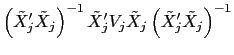
![LaTex Encoded Math: \displaystyle E\left[ \frac{\partial F\left( \hat{g}Z_{i}+d_{2}\left( \hat{y}_{2i}-\hat{y}% _{1i}\right) \right) }{\partial Z_{i}}\right]](img65.gif)
![]()
![LaTex Encoded Math: \displaystyle E\left[ \frac{\partial F\left( \hat{g}Z_{i}+d_{2}\left( \hat{y}_{... ...}\right) \right) }{\partial \left( \hat{y}_{2i}-\hat{y}_{1i}\right) }% \right]](img67.gif)
![]()
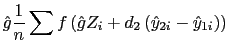
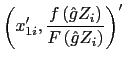
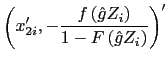
The second is the elasticity with respect to the independent variable, calculated as
![LaTex Encoded Math: \displaystyle E\left[ \frac{\partial F\left( \hat{g}Z_{i}+d_{2}\left( \hat{y}_{... ...( \hat{g}% Z_{i}+d_{2}\left( \hat{y}_{2i}-\hat{y}_{1i}\right) \right) }\right]](img69.gif)
![]()
![]()
In the case of a discrete independent variable, the marginal effect is calculated as

Conclusion
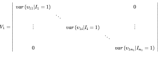
Standard error correction procedures
![]() and Murphy and Topel [1985].
and Murphy and Topel [1985].Ring time regression standard errors
![]()
![]()
![]()
![]()
![]()
![]()
![]()
![]()
Structural probit standard errors
![]() terms are predicted from the previous stage. This section outlines the method used, based on Murphy and Topel [1985].
terms are predicted from the previous stage. This section outlines the method used, based on Murphy and Topel [1985].![]() and and
and and
![]() on the subsamples that use debit cards and checks, respectively. However, the predicted values for
on the subsamples that use debit cards and checks, respectively. However, the predicted values for
![]() and
and
![]() are constructed for all observations. Thus, the log likehoods for the standard error correction procedure are different from those used to obtain the parameter vectors
are constructed for all observations. Thus, the log likehoods for the standard error correction procedure are different from those used to obtain the parameter vectors
![]() and
and
![]() Furthermore, the constructed term
Furthermore, the constructed term
![]() equals
equals![]()
![]() does not contain the selection terms.
does not contain the selection terms.
![]() observations. There is only one log-likelihood function for the second stage, which is
observations. There is only one log-likelihood function for the second stage, which is
![]() and let
and let
![]()
![]() According to Murphy and Topel [1985], the following formulation is a consistent approximation to the covariance matrix:
According to Murphy and Topel [1985], the following formulation is a consistent approximation to the covariance matrix:
![]()
![]()
![]()
![]()
![]()

![]()
![]()
![]()
![]()
The appropriate partial derivatives of the likelihood function are

![]()

![]()

![]()


![]()
and

![]()
Evaluating these expressions at the values
![]() and
and
![]() yields the asymptotically correct covariance matrices.
yields the asymptotically correct covariance matrices.
Variable name
Definition
Check
Equals 1 if consumer used a check
Debit card
Equals 1 if consumer used a debit card
Ring time
Time in seconds from ringing the first line item
to the close of the cash drawer.
Items bought
Number of items in the transaction
Value of sale
Total value of all items in transaction, calculated as value
of items plus tax minus value of coupons, where applicable, in dollars
Manufacturer coupons
Number of manufacturer coupons tendered
Store coupons
Number of store coupons tendered (associated with loyalty card)
Cash back indicator
Equals 1 if consumer received cash back
Value of cash back
In dollars
Monday
Day of week transaction occurred
Tuesday
Day of week transaction occurred
Wednesday
Day of week transaction occurred
Thursday
Day of week transaction occurred
Friday
Day of week transaction occurred
Saturday
Day of week transaction occurred
Median household income1,2
Median household income in census tract (1999)
Age of householder
35-44Percent of households where householder is between 35-44 years old
Age of householder
45-54Percent of households where householder is between 45-44 years old
Age of householder
55-64Percent of households where householder is between 55-44 years old
Age of householder
65-74Percent of households where householder is between 65-44 years old
Age of householder
75 and overPercent of households where householder is over 75 years old
Education3
Education3
High schoolPercent of population where high school is the highest level completed.
Education3
Some collegePercent of population where either some college or an associate's degree is the highest level completed.
Education3
CollegePercent of population where college or graduate school is the highest level completed.
Married
Percent of population
Female head
Percent of households where the householder
with children under 18
is a female with children under 18
Nonwhite4
Percent of population not classified as " White".
Urban
Percent of census tract living in an urban area or urban cluster
Owner occupied
![]()
Percent of housing units in census tract that are owner occupied
N
Number of observations
Notes
1.
![]() Includes the income of the householder and all other individuals 15 years old and over
Includes the income of the householder and all other individuals 15 years old and over
in the household, whether they are related to the householder or not.
2.
![]() In most cases, the householder is the person, or one of the people,
In most cases, the householder is the person, or one of the people,
in whose name the home is owned, being bought, or rented.
3.
![]() Data on educational attainment are tabulated for the population
Data on educational attainment are tabulated for the population
25 years old and over. People are classified according to the
highest degree or level of school completed.
4.
![]() "White" is a person having origins in any of the original peoples of
"White" is a person having origins in any of the original peoples of
Europe, the Middle East, or North Africa. It includes people
who indicate their race as "White" or report entries such as Irish,
German, Italian, Lebanese, Near Easterner, Arab, or Polish.
![]()
Indicates data source and supplied definition is from the
U.S. Census Bureau, Census 2000 statistics.
![]()
Indicates data source and supplied definition is from the
Federal Financial Institutions Examination Council Census Data Software, 2000 statistics.
Mean
Standard
deviationMedian
Min
Max
Check
0.56
0.497
1
0
1
Debit card
0.44
0.497
0
0
1
Ring time
128
75
109
20
597
Items bought
16.658
15.521
12
1
160
(Items bought)2
518
1009
144
1
25,600
Value of sale
40.27
36.43
28.81
0.26
357.04
(Value of sale)2
2948.60
5931.54
829.73
0.07
127477.5
Manufacturer coupons
0.322
1.763
0
0
70
Store coupons
1.913
4.211
0
0
98
Value of cash back
6.73
32.958
0
0
505.41
Cash back indicator
0.17
0.375
0
0
1
Day of week
Monday0.134
0.341
0
0
1
Day of week
Tuesday0.129
0.335
0
0
1
Day of week
Wednesday0.135
0.341
0
0
1
Day of week
Thursday0.129
0.335
0
0
1
Day of week
Friday0.144
0.351
0
0
1
Saturday
0.181
0.385
0
0
1
Median household income
46,630
19,809
40,967
20,327
117,690
Age of householder
35-440.222
0.059
0.216
0.101
0.446
Age of householder
45-540.198
0.037
0.193
0.145
0.377
Age of householder
55-640.138
0.032
0.138
0.052
0.249
Age of householder
65-740.113
0.043
0.115
0.015
0.231
Age of householder
75 and over0.093
0.046
0.093
0.012
0.223
Education
High school0.241
0.082
0.255
0.076
0.386
Education
Some college0.335
0.072
0.326
0.166
0.567
Education
College0.284
0.183
0.239
0.051
0.688
Married
0.613
0.094
0.624
0.395
0.814
Female head with children under 18
0.06
0.032
0.056
0.016
0.22
Nonwhite
0.14
0.148
0.087
0
0.809
Urban
0.731
0.324
0.826
0
1
Owner occupied
0.705
0.138
0.729
0.346
0.953
Debit card
EstimateDebit card
Std.
error
(adj.)Debit card
Std.
error
(unadj.)Check
EstimateCheck
Std.
error
(adj.)Check
Std.
error
(unadj.)
Items bought
3.242
![]()
0.070
0.073
3.775
![]()
0.080
0.081
(Items bought)2
-0.001
0.001
0.001
-0.009
![]()
0.001
0.001
No. of manufac. coupons
3.533
![]()
0.291
0.307
4.082
![]()
0.235
0.238
Day of week
Monday1.770
1.347
1.415
0.732
1.776
1.795
Day of week
Tuesday1.535
1.377
1.445
3.247
![]()
1.785
1.804
Day of week
Wednesday2.583
1.362
1.430
5.408
![]()
1.769
1.788
Day of week
Thursday2.415
1.401
1.471
5.907
![]()
1.770
1.789
Day of week
Friday4.636
![]()
1.340
1.408
5.507
![]()
1.737
1.756
Day of week
Saturday0.961
1.251
1.314
3.333
![]()
1.653
1.671
Value of cash back
0.167
![]()
0.028
0.030
0.215
![]()
0.011
0.011
Selection term
-13.344
![]()
1.473
1.548
-1.160
2.097
2.119
Intercept
42.997
![]()
1.417
1.486
75.061
![]()
2.356
2.381
Adjusted R2
0.595
0.506
F-statistic
1436.2
1267.7
No. of observations
10,760
13,594
Debit card
EstimateDebit card
Std.
error
(adj.)Debit card
Std.
error
(unadj.)Check
EstimateCheck
Std.
error
(adj.)Check
Std.
error
(unadj.)
Items bought
0.041
![]()
0.001
0.001
0.032
![]()
0.001
0.001
(Items bought)2
1.98E
![]()
7.01E
![]()
7.07E
![]()
No. of manufac. coupons
0.017
![]()
0.002
0.002
0.016
0.001
0.001
Day of week
Monday0.008
0.011
0.011
-0.001
0.011
0.011
Day of week
Tuesday-0.004
0.012
0.012
0.016
0.011
0.011
Day of week
Wednesday0.012
0.012
0.012
0.026
![]()
0.011
0.011
Day of week
Thursday0.005
0.012
0.012
0.032
![]()
0.011
0.011
Day of week
Friday0.028
![]()
0.011
0.011
0.033
![]()
0.011
0.011
Day of week
Saturday0.004
![]()
0.011
0.011
0.022
![]()
0.010
0.010
Value of cash back
0.002
![]()
2.47E
![]()
2.47E
![]()
0.001
![]()
6.98E
![]()
7.07E
![]()
Selection term
-0.134
![]()
0.013
0.012
-0.000
0.013
0.013
Intercept
3.890
![]()
0.012
0.012
4.357
![]()
0.015
0.015
Adjusted R2
0.609
0.515
F-statistic
1522.04
1313.67
No. of observations
10,760
13,594
Debit
EstimateDebit
Std.
error
(adj.)Debit
Std.
error
(unadj.)Check
EstimateCheck
Std.
error
(adj.)Check
Std.
error
(unadj.)
Items bought, log
0.342
![]()
0.004
0.004
0.333
![]()
0.004
0.004
No. of manufac. coupons
0.036
![]()
0.002
0.002
0.024
![]()
0.001
0.001
Day of week
Monday-0.003
0.012
0.012
-0.018
0.012
0.011
Day of week
Tuesday-0.016
0.012
0.012
0.003
0.012
0.011
Day of week
Wednesday-0.002
0.012
0.012
0.011
0.011
0.011
Day of week
Thursday-0.009
0.012
0.012
0.023
![]()
0.011
0.011
Day of week
Friday0.028
![]()
0.012
0.012
0.027
![]()
0.011
0.011
Day of week
Saturday0.002
0.011
0.011
0.022
0.011
0.011
Value of cash back
0.003
![]()
2.46E
![]()
2.47E
![]()
0.001
![]()
0.000
0.000
Selection term
-0.185
![]()
0.013
0.013
0.022
0.013
0.013
Intercept
3.574
![]()
0.013
0.013
4.016
![]()
0.018
0.017
Adjusted R2
0.581
0.487
F-statistic
1495.20
1290.49
No. of observations
10,760
13,594
Check
Debit card
Difference
Percent
differenceLog
difference
Mean
139.4
100.6
38.8
30.6
0.37
Median
122.5
83.5
38.7
31.8
0.38
Min
78.8
46.2
-80.7
-17.9
-0.07
Max
530.5
530.6
84.5
42.6
0.92
Check
Debit card
Difference
Percent
differenceLog
difference
Items bought
0-1089.02
53.80
35.22
0.397
0.454
Items bought
10.01-20.095.04
59.13
35.90
0.378
0.441
Items bought
20.01-30.0100.36
63.80
36.56
0.365
0.430
Items bought
30.01-40.0109.69
72.01
37.69
0.344
0.412
Items bought
40.01-50.0120.31
81.56
38.75
0.322
0.391
Items bought
50.01-60.0131.03
91.26
39.78
0.304
0.372
Items bought
60.01-70.0145.08
104.18
40.90
0.282
0.347
Items bought
70.01-80.0165.54
123.37
42.17
0.255
0.316
Items bought
80.01-90.0195.53
152.43
43.10
0.221
0.276
Items bought
90.01-100.0257.57
217.87
39.70
0.159
0.238
Manufac. coupons
0-92.0134.81
96.19
38.63
0.311
0.375
Manufac. coupons
92.01-96.0185.18
143.76
41.43
0.240
0.310
Manufac. coupons
96.01-100.0242.64
199.03
43.61
0.194
0.265
Cash back
0-84.0140.85
102.16
38.69
0.302
0.370
Cash back
84.01-90.0120.51
82.58
37.93
0.335
0.399
Cash back
90.01-100.0138.55
97.85
40.69
0.319
0.356
Use a debit card
EstimateUse a debit card
Std.
error
(adj.)Marginal effects
Mean
derivativeMarginal effects
Mean
elasticity
Value sale
-0.006
![]()
0.002
-0.002
-0.236
(Value sale)2
1.35E
![]()
4.69E
![]()
4.77E
![]()
0.043
No. of store coupons
-0.014
![]()
0.004
-0.005
-0.032
Median household income
7.16E
![]()
2.04E
![]()
2.54E
![]()
0.283
Age of householder
35 to 44-1.125
![]()
0.351
-0.399
-0.223
Age of householder
45 to 54-2.075
![]()
0.377
-0.736
-0.375
Age of householder
55 to 641.762
![]()
0.464
0.625
0.231
Age of householder
65 to 74-3.920
![]()
0.503
-1.390
-0.441
Age of householder
75 and over-1.468
![]()
0.386
-0.520
-0.139
High school
0.581
0.354
0.206
0.140
Some college
1.613
![]()
0.149
0.572
0.489
College
1.369
![]()
0.200
0.485
0.308
Married
0.027
0.231
0.010
0.015
Female head
1.614
![]()
0.546
0.572
0.095
Nonwhite
0.139
0.085
0.049
0.019
Urban
0.121
![]()
0.041
0.043
0.077
Owner occupied
-0.006
0.130
-0.002
-0.004
Cash back indicator
0.074
0.041
0.026
Time difference
-0.037
![]()
0.019
-0.013
-1.373
Intercept
0.871
0.734
0.309
0.808
Pseudo R2
0.095
Likelihood ratio
3,187.1
No. of observations
24,354
Use a debit card
EstimateUse a debit card
Std.
error
(adj.)Marginal effects
Mean
derivativeMarginal effects
Mean
elasticity
Value sale
-0.003
![]()
0.001
-0.001
-0.106
(Value sale)2
1.84E
![]()
7.10E
![]()
6.51E
![]()
0.058
No. of store coupons
-0.007
![]()
0.003
-0.003
-0.016
Median household income
7.22E
![]()
2.04E
![]()
2.56E
![]()
0.285
Age of householder
35 to 44-1.152
![]()
0.350
-0.408
-0.229
Age of householder
45 to 54-2.056
![]()
0.376
-0.729
-0.372
Age of householder
55 to 641.682
![]()
0.460
0.596
0.221
Age of householder
65 to 74-3.886
![]()
0.503
-1.377
-0.437
Age of householder
75 and over-1.500
![]()
0.382
-0.532
-0.143
High school
0.642
0.354
0.227
0.155
Some college
1.573
![]()
0.147
0.557
0.477
College
1.374
![]()
0.200
0.487
0.309
Married
0.007
0.230
0.002
0.004
Female head
1.627
![]()
0.545
0.577
0.096
Nonwhite
0.123
0.085
0.044
0.017
Urban
0.119
![]()
0.040
0.042
0.075
Owner occupied
-0.021
0.130
-0.008
-0.014
Cash back indicator
0.084
![]()
0.028
0.030
Time difference
3.218
![]()
0.358
1.141
1.061
Intercept
-1.898
![]()
0.236
-0.673
-1.761
Pseudo R2
0.095
Likelihood ratio
3,187.2
No. of observations
24,354
Use a debit card
EstimateUse a debit card
Std.
error
(adj.)Marginal effects
Mean
derivativeMarginal effects
Elasticity
Value sale
-0.011
![]()
0.001
-0.004
-0.467
(Value sale)2
4.63E
![]()
3.64E
![]()
1.65E
![]()
0.147
No. of store coupons
-0.012
![]()
0.003
-0.004
-0.028
Median household income
7.35E
![]()
2.04E
![]()
2.62E
![]()
0.290
Age of householder
35 to 44-1.194
![]()
0.350
-0.425
-0.237
Age of householder
45 to 54-2.100
![]()
0.375
-0.747
-0.379
Age of householder
55 to 641.725
![]()
0.459
0.614
0.226
Age of householder
65 to 74-3.894
![]()
0.502
-1.385
-0.437
Age of householder
75 and over-1.546
![]()
0.381
-0.550
-0.147
High school
0.667
0.353
0.237
0.160
Some college
1.642
![]()
0.147
0.584
0.498
College
1.427
![]()
0.199
0.508
0.320
Married
0.033
0.229
0.012
0.019
Female head
1.723
![]()
0.544
0.613
0.101
Nonwhite
0.123
0.085
0.044
0.017
Urban
0.112
![]()
0.040
0.040
0.071
Owner occupied
-0.026
![]()
0.130
-0.009
-0.017
Cash back indicator
0.087
![]()
0.028
0.031
Time difference
1.815
![]()
0.283
0.646
0.693
Intercept
-1.235
![]()
0.216
-0.439
-1.144
Pseudo R2
0.092
Likelihood ratio
3,083.7
No. of observations
24,354
Occupation
Hourly earnings
(in dollars)Shadow values
CheckShadow values
Debit cardShadow values
Difference
Cashier
7.65
0.28
0.19
0.08
Blue-collar
13.75
0.50
0.35
0.15
Physician
60.14
2.19
1.52
0.66
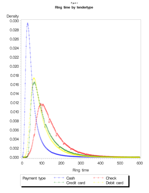
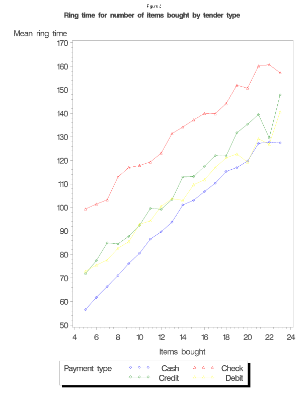
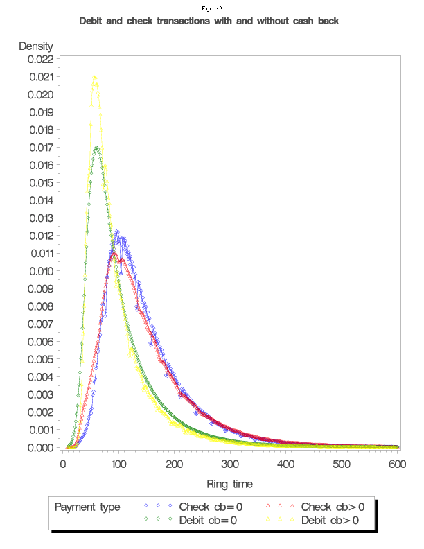
Bibliography
![]() , 19-31.
, 19-31.
Footnotes