Realized Jumps on Financial Markets and Predicting Credit Spreads*
Keywords: Jump-Diffusion Process, Realized Variance, Bi-Power Variation, Realized Jumps, Jump Volatility, Credit Risk Premium.
Abstract:
This paper extends the jump detection method based on bi-power variation to identify realized jumps on financial markets and to estimate parametrically the jump intensity, mean, and variance. Finite sample evidence suggests that jump parameters can be accurately estimated and that the statistical inferences can be reliable, assuming that jumps are rare and large. Applications to equity market, treasury bond, and exchange rate reveal important differences in jump frequencies and volatilities across asset classes over time. For investment grade bond spread indices, the estimated jump volatility has more forecasting power than interest rate factors and volatility factors including option-implied volatility, with control for systematic risk factors. A market jump risk factor seems to capture the low frequency movements in credit spreads.
JEL Classification Numbers: C22, G13, G14.1 Introduction
The relatively large credit spreads on high grade investment bonds has long been an anomaly in financial economics. Historically, firms that issue such bonds appear to entail very little default risk yet their credit spreads are sizable and positive (Huang and Huang, 2003). A natural explanation is that these firms are exposed to large sudden and unforeseen movements in the financial markets. In other words, the spread accounts for exposure to market jump risk. Jump risk has been proposed before as a possible source of the credit premium puzzle (Zhou, 2001; Huang and Huang, 2003; Delianedis and Geske, 2001), but the empirical validation in the literature has met with mixed and inconclusive results (Collin-Dufresne, Goldstein, and Helwege, 2003; Cremers, Driessen, Maenhout, and Weinbaum, 2005; Collin-Dufresne, Goldstein, and Martin, 2001; Cremers, Driessen, Maenhout, and Weinbaum, 2004). In this paper, we develop a jump risk measure based on identified realized jumps (as opposed to latent or implied jumps) as an explanatory variable for high investment grade credit spread indices.
The continuous-time jump-diffusion modeling of asset return process has a long history in finance, dating back to at least Merton (1976). However, the empirical estimation of the jump-diffusion processes has always been a challenge to econometricians. In particular, the identification of actual jumps is not readily available from the time-series data of underlying asset returns. Most of the econometric work relies on complicated numerical methods, or numerically intensive simulation-based procedures, and/or joint identification schemes from both the underlying asset and the derivative prices (see, e.g., Bates, 2000; Andersen, Benzoni, and Lund, 2002; Eraker, Johannes, and Polson, 2003; Pan, 2002; Chernov, Gallant, Ghysels, and Tauchen, 2003, among others).
This paper takes a different and direct approach to identify the realized jumps based on the seminal work by Barndorff-Nielsen and Shephard (2006,2004b). Recent literature suggests that the realized variance measure from high frequency data provides an accurate measure of the true variance of the underlying continuous-time process (Barndorff-Nielsen and Shephard, 2004a; Andersen, Bollerslev, Diebold, and Labys, 2003b; Meddahi, 2002). Within the realized variance framework, the continuous and jump part contributions can be separated by comparing the difference between realized variance and bi-power variation (see, Andersen, Bollerslev, and Diebold, 2004; Huang and Tauchen, 2005; Barndorff-Nielsen and Shephard, 2004b). Other jump detection methods have been proposed in the literature based on the swap variance contract (Jiang and Oomen, 2005), the range statistics (Christensen and Podolski, 2006), and the local volatility estimate (Lee and Mykland, 2006). Under the reasonable presumption that jumps on financial markets are usually rare and large, we assume that there is at most one jump per day and that the jump dominates the daily return when it occurs. This allows us to filter out the realized jumps, and further to directly estimate the jump distributions (intensity, mean, and variance). Such an estimation strategy based on identified realized jumps stands in contrast with existing literature that generate noisy parameter estimates based on daily returns.
Aït-Sahalia (2004) examines how to estimate the Brownian motion component by maximum likelihood, while treating the Poisson or Lévy jump component as a nuisance or noise. Our approach is exactly the opposite -- we estimate the jump component directly and then use the results for further economic analysis. The advantages of this approach include that we do not require the specification and estimation of the underlying drift and diffusion functions and that the jump process can be flexible. Such a jump detection and estimation strategy could be invalid for certain highly active Lévy process with infinite small jumps in a finite time period (Carr and Wu, 2004; Barndorff-Nielsen and Shephard, 2001; Bertoin, 1996). The approach here is more applicable to the compound Poisson jump process, where rare and potentially large jumps in financial markets are presumably the responses to significant economic news arrivals (Merton, 1976).
In Monte Carlo work, we examine two main settings where the jump contribution to total variance is 10% and 80%. In these situations, our realized jump identification approach performs well, in that the parameter estimates are accurate and converge as the sample size increases (long-span asymptotics). One important caveat is that these convergence results depend on choosing appropriately the level of the jump detection test. The significance level needs to be set rather loosely at 0.99 when jump contribution to total variance is low (10%), but set rather tightly at 0.999 when the jump contribution is high (80%). Note that a smaller jump contribution like 10% seems to be the main empirical finding in the literature (see, Andersen, Bollerslev, and Diebold, 2004; Huang and Tauchen, 2005, e.g.).
The proposed jump detection mechanism is implemented for the S&P500 market index, the 10-year US treasury bond, and the Dollar/Yen exchange rate, to cover a representative spectrum of asset classes. The jump intensity is estimated to be smallest for the equity index (13%), but larger for government bond (18%) and exchange rate (20%), while the jump mean estimates are insignificantly different from zero. The jump volatility estimates are for the stock market (0.54%), the bond market (0.65%), and the currency market (0.39%). Rolling estimates reveal interesting jump dynamics. The jump probabilities are quite variable for equity index and treasury bond (from 5% to 25%), but relatively stable for Dollar/Yen currency (20%). Although the jump means are mostly indistinguishable from zero for all assets considered here, there are obvious deviations from zero for the S&P500 index in late 1990s. Finally, the jump volatilities have not changed much for government bonds, except for a hike in 1994, and the exchange rate, but have increased significantly for the US equity market from 2000 to 2004.
It turns out that the capability to identify realized jumps has important implications for estimating financial market risk adjustments. For the Moody's AAA and BAA credit spread indices, we find that the rolling estimates of stock market jump volatility can predict the spread variation with R-squares of 0.65 and 0.72, which are considerably higher than obtained with the standard interest rate factors, volatility factors including the option-implied volatility, and the systematic Fama-French factors. This result is important, since explaining high investment grade credit spreads has not been very successful and the empirical role of jumps in explaining these credit spreads has not been largely confirmed in literature so far. This evidence is also consistent with the finding in Zhang, Zhou, and Zhu (2005) that credit spreads of individual firms are well explained by the realized jump risk measures estimated similarly from high frequency individual equity prices.
The rest of the paper is organized as follows: the next section introduces the jump identification mechanism based on high frequency intraday data, then Section 3 provides some Monte Carlo evidence on the small sample performance of such an estimation strategy. Section 4 illustrates the approach with four financial market assets, Section 5 discusses the implications for predicting credit risk spreads, and Section 6 concludes.
2 Identifying Realized Jumps
Jumps are important for asset pricing (Merton, 1976), yet the estimation of jump distribution is very difficult, especially when only low frequency daily data are employed (Andersen, Benzoni, and Lund, 2002; Bates, 2000; Aït-Sahalia, 2004; Chernov, Gallant, Ghysels, and Tauchen, 2003; Pan, 2002; Eraker, Johannes, and Polson, 2003). In recent years, Andersen and Bollerslev (1998), Andersen, Bollerslev, and Diebold (2005b); Andersen, Bollerslev, Diebold, and Labys (2001), Barndorff-Nielsen and Shephard (2002b,a), and Meddahi (2002), have advocated the use of so-called realized variance measures by utilizing the information in the intra-day data for measuring and forecasting volatilities. More recent work on bi-power variation measures developed in a series of papers by Barndorff-Nielsen and Shephard (2006,2003,2004b) allows for the use of high-frequency data to disentangle realized volatility into separate continuous and jump components (see, Andersen, Bollerslev, and Diebold, 2004; Huang and Tauchen, 2005, as well). In this paper, we rely on the presumption that jumps on financial markets are rare and large in order to extract the realized jumps and to explicitly estimate the jump intensity, mean, and volatility parameters. Empirical evidence presented by Lee and Mykland (2006, Table V) is generally supportive of the notion of very rare jumps.
2.1 Filtering Jumps from Bi-Power Variation
Let
![]() denotes the time
denotes the time ![]() logarithmic price of the asset, and it evolves in
continuous time as a jump diffusion process:
logarithmic price of the asset, and it evolves in
continuous time as a jump diffusion process:
| (1) |
where
| (2) |
where
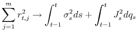
Barndorff-Nielsen and Shephard (2004b) propose two general measures for the quadratic variation process--realized variance and realized bi-power variation--which converge uniformly (as
![]() or
or
![]() ) to different quantities of the underlying jump-diffusion process,
) to different quantities of the underlying jump-diffusion process,
 |
(3) | ||
 |
(4) |
Therefore the difference between the realized variance and bi-power variation is zero when there is no jump and strictly positive when there is a jump (asymptotically).
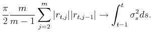
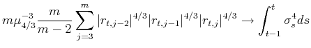
A variety of jump detection techniques are proposed and studied by Barndorff-Nielsen and Shephard (2004b), Andersen, Bollerslev, and Diebold (2004), and Huang and Tauchen (2005). Here we adopted the ratio statistics
favored by their findings,
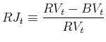 |
(5) |
which converges to a standard normal distribution with appropriate scaling
![\displaystyle ZJ_t \equiv \frac{RJ_t}{\sqrt{[(\frac{\pi}{2})^2+\pi-5] \frac{1}{m}\max(1,\frac{TP_t}{BV_t^2})}} \stackrel{d}{\longrightarrow} {\cal N} (0, 1)](img29.gif) |
(6) |
where
 |
(7) |
with
Based on the economic intuition regarding the nature and source of jumps on financial market (Merton, 1976), we further assume that there is at most one jump per day and that the jump size dominates the return when a jump occurs. These assumptions allow us to filter out
the daily realized jumps as
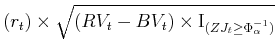 |
(8) |
where
2.2 Estimating the Jump Distribution
Once the individual jump size is filtered out, we can further estimate the jump intensity, mean, and variance, by imposing a simple model of Poisson-mixing-Normal jump specification,
 |
|||
with appropriate formulas for the standard error estimates. Such an approach for estimating jumps is robust to the specifications of time-varying or even stochastic drift and diffusion functions, as long as the diffusion volatility noise is not too large (to be made more precise in the Monte Carlo study of the next section). It also allows us to specify more flexible dynamic structures of the underlying jump arrival rate and/or jump size distribution (see, for example, Andersen, Bollerslev, and Huang, 2006). Realized jumps therefore can help us to avoid those estimation methods such as EMM or MCMC that rely heavily on numerical simulations.
2.3 Pre-Test Level and Noise-to-Signal Ratio
There appears to be no conclusive agreement about the optimal significance level ![]() of the jump-detection
of the jump-detection ![]() -test in various empirical settings (Andersen, Bollerslev, and Diebold, 2004; Huang and Tauchen, 2005;
Barndorff-Nielsen and Shephard, 2004b). However, our finite sample evidence presented bellow suggests that when relative jump contribution to total variance is small (10%) a more generous test level (
-test in various empirical settings (Andersen, Bollerslev, and Diebold, 2004; Huang and Tauchen, 2005;
Barndorff-Nielsen and Shephard, 2004b). However, our finite sample evidence presented bellow suggests that when relative jump contribution to total variance is small (10%) a more generous test level (
![]() ) performs better, while for large jump contribution (80%) a more stringent test level (
) performs better, while for large jump contribution (80%) a more stringent test level (
![]() ) is preferred. This relationship may be formalized as determined by a "noise-to-signal" in identifying jumps, with the presence of diffusion as a measurement error. More
precisely, the ratio of unconditional expectations of
) is preferred. This relationship may be formalized as determined by a "noise-to-signal" in identifying jumps, with the presence of diffusion as a measurement error. More
precisely, the ratio of unconditional expectations of
![]() over
over ![]() ,
,
 |
(9) |
appears to indicate the optimal choice of the test level
2.4 When Jumps Are not so Large and Rare
The assumption of large jumps is rather innocuous, as long as jumps remain discretely distinct from the continuous diffusion, and therefore higher sampling frequency can eventually capture the jumps. The resulting estimates of jump parameters becomes more noisy but have no asymptotic bias as both sample size increases and sampling interval decreases. However, more frequent jumps might distort the finite sample properties and cause bias.
3 Finite Sample Experiment
It is important to evaluate whether the proposed jump filtering and estimation procedure works well under the assumptions of large and rare jumps. In particular, we want to know whether the jump parameters can be accurately estimated and whether the correct inferences can be made, as both the sample size increases and the sampling interval decreases.
3.1 Experimental Design
Here we adopt the following benchmark specification of a stochastic volatility jump-diffusion process,
| (10) | |||
| (11) |
with log price drift
The Monte Carlo experiment is designed as follows. Each day one simulates the jump-diffusion process, using 1-second as a tick size totaling six and a half trading hours, imitating the US equity market in recent years. The diffusion process with stochastic volatility is simulated by the Euler
scheme, the jump timing is simulated from an Exponential distribution, and the jump size is simulated from a Normal distribution. Then the realized jumps are combined with the realized diffusion, and sampled by an econometrician at both 1-minute and 5-minute intervals, illustrating the in-fill
asymptotics. To contrast the long-span asymptotics of sample sizes, we use both T = 1000 days and T = 4000 days. Further, the choice of significance level in the jump detection test is also compared between
![]() and
and
![]() . The appropriate choice of the pre-test level seems to be relevant for achieving consistent parameter estimates, given varying degree of jump contribution to the total variance.
In addition, the simulation provides us the exact jump timing (Exponential) and jump size (Normal), therefore a maximum likelihood estimator (MLE) can be used as a benchmark for judging the relative efficiency of the jump filtering approach examined in this paper.
. The appropriate choice of the pre-test level seems to be relevant for achieving consistent parameter estimates, given varying degree of jump contribution to the total variance.
In addition, the simulation provides us the exact jump timing (Exponential) and jump size (Normal), therefore a maximum likelihood estimator (MLE) can be used as a benchmark for judging the relative efficiency of the jump filtering approach examined in this paper.
3.2 Parameter Estimation
The finite sample results on various jump parameter estimates are presented in Tables 1-2. The first column of each table gives the true parameter values, and the first row gives the mean bias, median bias, and root-mean-squared-error (RMSE) of the maximum likelihood estimator (MLE). Note that
the MLE results do not vary across the two scenarios (since only the diffusion variance level is altered), nor across the pre-test
![]() and
and
![]() levels (since no pre-estimation filtering is involved), nor across the 5-minute and 1-minute sampling intervals (since jumps are observed exactly in simulations). For MLE, the
estimation biases at both 1000 and 4000 days are negligible for all three parameters, relative to their true values. In terms of the estimation efficiency, both jump rate
levels (since no pre-estimation filtering is involved), nor across the 5-minute and 1-minute sampling intervals (since jumps are observed exactly in simulations). For MLE, the
estimation biases at both 1000 and 4000 days are negligible for all three parameters, relative to their true values. In terms of the estimation efficiency, both jump rate ![]() and jump
volatility
and jump
volatility ![]() can be very accurately estimated with RMSE's much smaller than the parameter values. However, for the jump mean parameter
can be very accurately estimated with RMSE's much smaller than the parameter values. However, for the jump mean parameter ![]() , the estimate is not accurate at 1000 days (RMSE about the size of parameter value), but can be accurate at 4000 days (RMSE about half the size of parameter value). In addition, all the RMSE's decrease almost exactly at the rate of
, the estimate is not accurate at 1000 days (RMSE about the size of parameter value), but can be accurate at 4000 days (RMSE about half the size of parameter value). In addition, all the RMSE's decrease almost exactly at the rate of
![]() , as predicted by the asymptotic theory.
, as predicted by the asymptotic theory.
For the jump filtering mechanism based on the bi-power variation measure (Tables 1-2), the parameter estimation efficiency approaches that of MLE very differently, depending upon whether the jump contribution to total variance is small or large. In Scenario (a) where the jump contribution to
total variance is as small as 10%, the RMSE's of parameter estimates are all closer to those of MLE and the convergence rates are closer to ![]() , as the sample size increases from T =
1000 to T = 4000, when we set the pre-test level
, as the sample size increases from T =
1000 to T = 4000, when we set the pre-test level
![]() but not
but not
![]() . In other words, when the jump contribution is relatively small as is typical in observed data, the asymptotic filtering scheme seems to work better when the pre-test level is
less stringent. In contrast, for Scenario (b) where the jump contribution to total variance is as large as 80%, the scheme seems to work much better when we set
. In other words, when the jump contribution is relatively small as is typical in observed data, the asymptotic filtering scheme seems to work better when the pre-test level is
less stringent. In contrast, for Scenario (b) where the jump contribution to total variance is as large as 80%, the scheme seems to work much better when we set
![]() rather than
rather than
![]() , where the RMSE's can almost match those of MLE. These findings are intuitive in the following sense. It is clearly more difficult to detect jumps when they are relatively small,
therefore loosening the jump detection standard can reveal more jumps that otherwise would have been missed (minimizing the type-I error). On the other hand, when jumps are large they are easier to detect, so we want a more stringent jump filtering standard, such that false revelation of jumps can
be avoided as much as possible (minimizing the type-II error). In short, the jump filtering approach based on the bi-power variation measure can bring us efficient parameter estimates relative to MLE, provided that we appropriately choose the significance level
, where the RMSE's can almost match those of MLE. These findings are intuitive in the following sense. It is clearly more difficult to detect jumps when they are relatively small,
therefore loosening the jump detection standard can reveal more jumps that otherwise would have been missed (minimizing the type-I error). On the other hand, when jumps are large they are easier to detect, so we want a more stringent jump filtering standard, such that false revelation of jumps can
be avoided as much as possible (minimizing the type-II error). In short, the jump filtering approach based on the bi-power variation measure can bring us efficient parameter estimates relative to MLE, provided that we appropriately choose the significance level ![]() according to the relative contributions of jumps to total variance.
according to the relative contributions of jumps to total variance.
3.3 Statistical Inference
In addition to the parameter estimation efficiency, we also need to know whether the asymptotic standard error estimated in finite samples can provide a reliable statistical inference about the true parameter value. To set the right benchmark, Figure 1 plots the finite sample rejection rates from the Monte Carlo replications against the asymptotic test size. The rejection rate is based on the Chi-square (1) test statistics of each parameter. The deviation between the dashed line (Monte Carlo finite sample result) and dotted diagonal line (asymptotic result), indicates how big is the size distortion. It is clear from Figure 1 that the MLE asymptotic variance estimated in finite sample behaves extremely well, so there is effectively no size distortion at all.
The Wald test statistics based on bi-power variation approach are reported in Figures 2-3. In general, the ![]() -test for the jump mean
-test for the jump mean ![]() is well behaved, while the result for jump rate
is well behaved, while the result for jump rate ![]() and jump volatility
and jump volatility ![]() varies with the setting. In Scenario (a) where jumps contribute 10% to total variance, the chi-square statistics under the choice of
varies with the setting. In Scenario (a) where jumps contribute 10% to total variance, the chi-square statistics under the choice of
![]() have a much higher over-rejection bias compared to the choice of
have a much higher over-rejection bias compared to the choice of
![]() . In Scenario (b) with relative jump contribution being 80%, there is almost no over-rejection bias at
. In Scenario (b) with relative jump contribution being 80%, there is almost no over-rejection bias at
![]() level, while the chi-square test does not converge at all for
level, while the chi-square test does not converge at all for
![]() . In short, if jumps are small then less stringent jump detection test generates more reliable inferences about the true parameters, while if jumps are large then more stringent
test generates more reliable inferences.
. In short, if jumps are small then less stringent jump detection test generates more reliable inferences about the true parameters, while if jumps are large then more stringent
test generates more reliable inferences.
4 Application to Financial Markets
We apply the jump detecting and filtering scheme to three financial markets: stocks, bonds, and foreign exchange. The intraday high frequency data for S&P500 index (1986-2005) is obtained from the Institute of Financial Market, the 10-year US treasury bond (1991-2005) from the Federal Reserve Board, and the Dollar/Yen exchange rate (1997-2004) from Olsen & Associates. These choices are meant to give a representative view of the available major asset classes. All the data are transformed to five minute log returns, which are generally known to be quite robust to market microstructure noise. We eliminate days with less than 60 trades or quotes. We also drop the after-hour tradings due to the liquidity concern, except for the Dollar/Yen exchange rate, which opens for 24 hours.
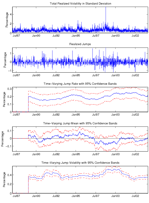
Summary statistics for daily percentage returns and realized volatility (square-root of realized variance) are reported in Table 3. The sample means suggest annualized returns of 8.7% for the S&P 500, 4.1% for the t-bond, and 2.4% for Yen currency (six trading days per week). The average realized volatilities are for the stock market index 0.73%, the t-bond 0.56%, and the exchange rate 0.62%. The return skewness is negative for S&P 500 index and government bond, while positive for exchange rate. The kurtosis statistics suggests all three returns deviate from the Normal distribution, as is expected. The returns are approximately serially uncorrelated, while the volatility series exhibit pronounced serial dependencies. In fact, the first ten autocorrelations reported in the bottom part of the table are all highly significant with the gradual, but very slow, decay suggestive of long-memory type features. This is also evident from the time series plots of realized volatility series given in the top panels of Figures 4-6.
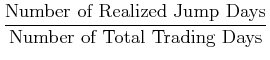
4.1 Unconditional Jump Parameter Estimates
As shown in the top panel of Table 4, the jump contribution to total variance is about 5.28% for S&P500, 19.11% for t-bond, and 6.47% for the exchange rate. These numbers are very close to the findings in Andersen, Bollerslev, and Diebold (2004) and Huang and Tauchen (2005), and quite similar to Scenario (a) of our Monte Carlo section. We expect the jump filtering and estimation method based on the bi-power variation approach to work reasonably well. The realized jumps filtered by our method are plotted in the second panels of Figures 4-6. Jumps in S&P 500 index clearly have jump sizes between -2% and +2%. Treasury bond has less frequent jumps with a range -2% and +4%. The Yen currency has more frequent jumps with jump size between -1.2% and +1.6%.
The bottom panel of Table 4 reports the parametric distribution estimates based on the filtered realized jumps. Except for the S&P 500 index (![]() = 0.05 with s.e. = 0.02), all the
jump mean estimates are statistically indistinguishable from zero. The jump intensity estimates are highly significant and vary across assets, with the S&P 500 index being the lowest (0.13 with s.e. 0.01), the Treasury bond moderate (0.18 with s.e. 0.02), and the exchange rate the highest (0.20
with s.e. 0.01). The standard deviations of jumps are estimated the most accurately and very close to each other (0.55 with s.e. 0.02 for the stock index, 0.65 with s.e. 0.02 for bond, and 0.39 with s.e. 0.01 for currency).
= 0.05 with s.e. = 0.02), all the
jump mean estimates are statistically indistinguishable from zero. The jump intensity estimates are highly significant and vary across assets, with the S&P 500 index being the lowest (0.13 with s.e. 0.01), the Treasury bond moderate (0.18 with s.e. 0.02), and the exchange rate the highest (0.20
with s.e. 0.01). The standard deviations of jumps are estimated the most accurately and very close to each other (0.55 with s.e. 0.02 for the stock index, 0.65 with s.e. 0.02 for bond, and 0.39 with s.e. 0.01 for currency).
These results differ from the usual jump estimation results in empirical finance that use latent variable simulation-based methods on daily data. Our findings regarding jump frequency and jump size can be reconciled with the notion that significant jumps on financial markets are related to market responses to fundamental economic news (Andersen, Bollerslev, Diebold, and Vega, 2003a,2005a).
4.2 Time-Varying Jump Distribution Estimates
Another interesting feature that can be seen from the second panels of Figures 4-6, is that the clustering and amplitude of jumps change over time, which leads to the usual conjecture of time-varying jump rate and jump size distribution. To get an initial handle of such a possibility, we perform
a two-year rolling estimation of the jump parameters
![]() ,
, ![]() , and
, and
![]() , with corresponding 95% standard error bands.
, with corresponding 95% standard error bands.
As seen from Figure 4, the jump intensity of S&P 500 index was fairly high during the early 1990s (above 20%), then dropped considerably during the late 1990s (around 5%), and has started to rise again since 2002. The jump size mean is usually close to zero, except for the during late 1990s, where positive jump means are statistically significant and coinciding with the stock market run-up. Jump volatility had been largely stable from the late 1980s to the late 1990s around 40%, but has been elevated since 1999 and peaked around 2002 at a high of 100%. As Figure 5 shows, the jump intensity of the bond market was high in the early 1990s and around 2001-2002, then kept falling until 2004 to around 10%; while jump mean is mostly zero and jump volatility is little changed around its unconditional level of 60% (except for the early 1990s when it is around 100%). For the Dollar/Yen exchange rate in Figure 6, jump intensity is mostly stable around 20%, jump mean is statistically indistinguishable from zero, and jump volatility is somewhat elevated during 1991-1992 and 1998-2000.
Time-varying jump intensity and jump volatility are very important risk factors in asset pricing, but until recently most of the evidence has been drawn from the option implied or latent jump specifications (see, for example, Eraker, Johannes, and Polson, 2003; Duffie, Pan, and Singleton, 2000, among others). A recent paper by Andersen, Bollerslev, and Huang (2006) use the realized jump timing to examine the temporal dependency in jump durations.
5 Jump Risks and Credit Spreads
Direct identification of realized jumps and the characterizations of time-varying jump distributions make it straightforward to study the relationship between jumps and risk adjustments. The reason is that jump parameters are generally very hard to pin down even with both underlying and derivative assets prices, due to the fact that jumps are latent in daily return data and are rare events in financial markets. Inaccurate estimates of the underlying jump dynamics makes the jump risk premia even harder to quantify. However, as seen bellow, a reliable estimate of stock market jump volatility based on identified realized jumps, can have a superior predicting power for the bond market risk premia.
5.1 Predicting Corporate Bond Spread Indices
Here we examine the daily forecasting powers for Moody's AAA and BAA bond spreads, using the estimated S&P 500 jump volatility from the identified realized jumps, which is illustrated in Section 4. A longstanding puzzle has been how to explain the credit spreads of high investment grade bonds, since those firms entertain very little default risk historically, yet their credit spreads are sizable and positive (Huang and Huang, 2003). Although jump risk has been proposed as a possible source of such a credit premium puzzle (Zhou, 2001; Huang and Huang, 2003; Delianedis and Geske, 2001), the empirical validation in literature has met with mixed and unsatisfactory results (Collin-Dufresne, Goldstein, and Helwege, 2003; Cremers, Driessen, Maenhout, and Weinbaum, 2005; Collin-Dufresne, Goldstein, and Martin, 2001; Cremers, Driessen, Maenhout, and Weinbaum, 2004). Here we use an alternative jump risk measure, based on identified realized jumps as opposed to latent or implied jumps, to provide some contrasting positive evidence in explaining high investment grade credit spread indices. For comparison purposes, we also include standard predictors like the short rate and term spread in Longstaff and Schwartz (1995), long-run historical volatility (Campbell and Taksler, 2003) and short-run realized volatility (Zhang, Zhou, and Zhu, 2005), and option implied volatility (Cao, Yu, and Zhong, 2006), with a control for market return, book-to-market, and size risk factors (Fama and French, 1993).
Table 5 presents the univariate forecasting regressions for Moody's AAA and BAA bond spreads indices. The OLS coefficients show remarkable similarity between the two rating grades. To be more precise, a one percentage increase in the short rate lowers credit spread 14 and 16 basis points;
positive term spread increases default premium 5 and 12 basis points. The short rate predicts 44% and 36% of spread variation, while the term spread by itself has very little forecasting power. Short-run volatility (1-day) has R![]() s around 30% with marginal impact around 4 basis points, while long-run volatility (2-year) has higher R
s around 30% with marginal impact around 4 basis points, while long-run volatility (2-year) has higher R![]() s, about 50-60%, and higher impact
coefficient of 7 to 9 basis points. It is worth pointing out that option implied volatility (VIX index) has about the same predicting power and marginal effect as the long-run and short-run volatilities. In comparison, the S&P 500 jump volatility not only has a larger impact on credit spreads
-- a one percentage point increase raises spreads about 150-190 basis points, but also has the highest forecasting power -- with R
s, about 50-60%, and higher impact
coefficient of 7 to 9 basis points. It is worth pointing out that option implied volatility (VIX index) has about the same predicting power and marginal effect as the long-run and short-run volatilities. In comparison, the S&P 500 jump volatility not only has a larger impact on credit spreads
-- a one percentage point increase raises spreads about 150-190 basis points, but also has the highest forecasting power -- with R![]() s of 65% for the AAA bond spread and 72% for the BAA bond
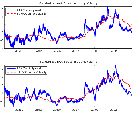
spread. The close association between credit risk premium and market jump volatility can be more clearly seen in Figure 7. Although the daily credit spread is very noisy, there clearly exist certain long term trends and short term cycles from 1988 to 2004. It is obvious that the time-varying jump
volatility traces closely these trends and cycles, while discarding the day-to-day fluctuations in credit spread indices.
s of 65% for the AAA bond spread and 72% for the BAA bond
spread. The close association between credit risk premium and market jump volatility can be more clearly seen in Figure 7. Although the daily credit spread is very noisy, there clearly exist certain long term trends and short term cycles from 1988 to 2004. It is obvious that the time-varying jump
volatility traces closely these trends and cycles, while discarding the day-to-day fluctuations in credit spread indices.
Given the common finding that typical default risk factors can only account for a very small fraction of the corporate bond spreads, recent effort has been directed more to the role of systematic risk premia in the economy (see, Chen, Collin-Dufresne, and Goldstein, 2005; Elton, Gruber, Agrawal, and Mann, 2001; Huang and Huang, 2003, e.g.). However, those business cycle effects usually explain only the spread variations of low investment grade or speculative grade credit spreads, but have very little or no explanatory power for the high investment grade credit spreads. As Table 6 shows, the systematic risk factors--market return, SMB, and HML Fama-French variables--have zero predictive ability for the high investment grade credit spread at the daily frequency. The fact that these bonds have little default risk yet command a sizable risk premium constitutes a major challenge in the credit risk pricing literature. In comparison, the jump volatility risk measure stands out as the most powerful instrument in forecasting the credit spread indices, suggesting that a systematic jump risk factor may be important in pricing the top quality corporate credit.
Table 7 presents multiple regressions in forecasting the bond spreads. It seems that two interest rate factors are complementary, in that the combined R![]() is much higher than the sum of
two univariate regressions. The signs of both short rate and term spread are now negative and larger. Intuitively, when the economy is in expansion, the short rate and term spread tend to be rising, and the credit default condition is also improving. Note that when combining short- and long-run
volatilities or implied and jump volatilities, the coefficient magnitude and significance level mostly remain the same. It suggests that two volatility components may be needed in explaining the risk premium dynamics (Adrian and Rosenberg, 2006). The last columns in Table 7
are the multiple regressions that reach R
is much higher than the sum of
two univariate regressions. The signs of both short rate and term spread are now negative and larger. Intuitively, when the economy is in expansion, the short rate and term spread tend to be rising, and the credit default condition is also improving. Note that when combining short- and long-run
volatilities or implied and jump volatilities, the coefficient magnitude and significance level mostly remain the same. It suggests that two volatility components may be needed in explaining the risk premium dynamics (Adrian and Rosenberg, 2006). The last columns in Table 7
are the multiple regressions that reach R![]() s around 80%.
s around 80%.
In short, contrary to the negative finding in the empirical literature about the jump impact on credit spread, our measure of market realized jump volatility has strong predictability for high investment grade credit spreads. The forecasting power is higher than the interest rate factors, short-run and long-run volatility factors, or even the option implied volatility factor, with controlling for the systematic risks of market return, SMB and HML.
5.2 Explaining Credit Default Spreads of Individual Firms
In a related paper, Zhang, Zhou, and Zhu (2005) apply the jump identification strategy of this paper to individual firms, and find that the realized jump risk measures (intensity, mean, and volatility) from firm level equity returns all have strong explanatory power for
credit default swap (CDS) spreads. In particular, jump risk alone can predict about 19% variation of the CDS spreads. By separating realized volatility and jump measures, they also strengthen the forecasting power of equity volatility measures as in Campbell and Taksler
(2003), and increase the overall forecasting R![]() to 77%. Furthermore, they find that the nonlinear effects of jump and volatility risk measures on credit spreads are largely consistent
with a structural model with stochastic volatility and jumps.
to 77%. Furthermore, they find that the nonlinear effects of jump and volatility risk measures on credit spreads are largely consistent
with a structural model with stochastic volatility and jumps.
6 Conclusion
Disentangling jumps from diffusion has always been a challenge for pricing financial assets and for estimating the jump-diffusion processes. Building on the recent jump detection literature for separating realized variance and bi-power variation (Andersen, Bollerslev, and Diebold, 2004; Barndorff-Nielsen and Shephard, 2006; Huang and Tauchen, 2005; Barndorff-Nielsen and Shephard, 2003,2004b), we extend the methodology to filter out the realized jumps, under two key assumptions typically adopted in financial economics: (1) jumps are rare and there is at most one jump per day, and (2) jumps are large and dominate return signs when they occur.
These approximations provide a powerful tool to identify the realized jumps on financial markets. Our Monte Carlo experiments under realistic empirical settings suggest that accurate parameter estimates and properly sized inference tests can be obtained with an appropriate choice of the significance level of the jump detection pre-test.
The proposed jump identification method is applied to three financial markets -- S&P 500 index, treasury bond, and Dollar/Yen exchange rate. We find that the jump intensity varies among these asset classes from 13% to 20%. All the jump mean estimates are insignificantly different from zero, except for the S&P 500 index driven by a positive run in late 1990s. Jump volatility is similar for the exchange rate (0.39%), the equity market (0.54%), and the bond market (0.65%). Rolling estimates reveal that the jump probabilities are quite variable for the equity index and treasury bonds (from 5% to 25%), but relatively stable for the Yen currency (20%). The jump volatility is little changed for government bonds (except for the run up in 1992-1994), while elevated a great deal for the stock market from 2000 to 2004 and moderately for the Dollar/Yen in early and late 1990s.
The identification of realized jumps and direct estimation of jump distributions has important implications in assessing financial market risk adjustments. Given more reliable estimates of the jump dynamics, the impact on jump risk premia can be more precisely quantified. For example, the Moody's AAA and BAA credit risk premia can be predicted by the realized jump volatility measure, much better than the by interest rate factors, volatility factors including option-implied volatility, and Fama-French risk factors. Explaining the credit spreads of high investment grade entities has always been a challenge in credit risk pricing, and a systematic jump risk factor holds some promise in resolving such an puzzle. Individual firm's credit spreads can also be better predicted by the realized jump risk measures from each firm's equity returns (Zhang, Zhou, and Zhu, 2005).
Bibliography
Working Paper.
Federal Reserve Bank of New York.
Journal of Financial Economics, 74, 487-528.
American Economic Review, 93, 38-62.
Working Paper.
University of Rochester.
Journal of Finance, 57, 1239-1284.
International Economic Review, 39, 885-905.
Working Paper.
Duke University.
Elsevier Science B.V., Amsterdam.
forthcoming.
Journal of the American Statistical Association, 96, 42-55.
Econometrica, 71, 579-625.
Working Paper.
Duke University.
Journal of the Royal Statistical Society, Series B, 63, 167-241.
Journal of Royal Statistical Society, Series B 64.
Journal of Applied Econometrics, 17, 457-478.
Bernoulli, 9, 243-165.
Econometrica, 72, 885-925.
Journal of Financial Econometrics, 2, 1-48.
Journal of Financial Econometrics, 4, 1-30.
Journal of Econometrics, 94, 181-238.
Cambridge University Press, Cambridge.
Journal of Finance, 58, 2321-2349.
Working Paper.
University of California, Irvine.
Journal of Financial Economics, 17, 113-141.
Working Paper.
Michigan State University.
Journal of Econometrics, 116, 225-258.
Working Paper.
Aarhus School of Business.
Working Paper.
Carnegie Mellon University.
Journal of Finance, 56, 2177-2207.
Yale ICF Working Paper.
Yale School of Management.
Working Paper.
Cornell University.
Working Paper.
Anderson Graduate School of Management, UCLA.
Econometrica, 68, 1343-1376.
Journal of Finance, 56, 247-277.
Journal of Finance, 53, 1269-1300.
Journal of Financial Eonomics, 33, 3-56.
Working Paper.
Journal of Financial Econometrics, 3, 456-499.
Working Paper.
Finance Department at University of Arizona.
Technical Report No. 566.
Department of Statistics, University of Chicago.
Journal of Finance, 50, 789-820.
Journal of Applied Econometrics, 17, 479-508.
Journal of Financial Economics, 3, 125-144.
Journal of Financial Economics, 63, 3-50.
Working Paper.
Federal Reserve Board.
Journal of Banking and Finance, 25, 2015-2040.
This table reports the Monte Carlo evidence for estimating the jump rate, mean, and volatility parameters. Scenario (a) has the jump contribution to total variance as 10%. The results are organized across two sample sizes (1000 days versus 4000 days), two sampling frequencies (5-minute versus 1-minute), and two jump test significance levels (0.99 versus 0.999).
| Mean Bias T = 1000 |
Mean Bias T = 4000 |
Medium Bias T = 1000 |
Medium Bias T = 4000 |
RMSE T = 1000 |
RMSE T = 4000 |
|
|---|---|---|---|---|---|---|
|
|
0.0006 | 0.0004 | 0.0005 | 0.0004 | 0.0068 | 0.0035 |
| -0.0020 | 0.0017 | -0.0060 | 0.0046 | 0.1989 | 0.1033 | |
|
|
-0.0094 | -0.0005 | -0.0042 | -0.0030 | 0.1443 | 0.0690 |
| Mean Bias T = 1000 |
Mean Bias T = 4000 |
Medium Bias T = 1000 |
Medium Bias T = 4000 |
RMSE T = 1000 |
RMSE T = 4000 |
|
|---|---|---|---|---|---|---|
|
|
-0.0065 | -0.0061 | -0.0070 | -0.0060 | 0.0092 | 0.0068 |
| -0.0131 | -0.0079 | -0.0147 | -0.0082 | 0.2152 | 0.1116 | |
|
|
-0.0116 | -0.0006 | -0.0126 | 0.0023 | 0.1443 | 0.0706 |
| Mean Bias T = 1000 |
Mean Bias T = 4000 |
Medium Bias T = 1000 |
Medium Bias T = 4000 |
RMSE T = 1000 |
RMSE T = 4000 |
|
|---|---|---|---|---|---|---|
|
|
-0.0006 | -0.0001 | 0.0000 | 0.0000 | 0.0067 | 0.0035 |
| -0.0239 | -0.0194 | -0.0233 | -0.0238 | 0.1965 | 0.1039 | |
|
|
-0.0464 | -0.0363 | -0.0550 | -0.0348 | 0.1504 | 0.0766 |
| Mean Bias T = 1000 |
Mean Bias T = 4000 |
Medium Bias T = 1000 |
Medium Bias T = 4000 |
RMSE T = 1000 |
RMSE T = 4000 |
|
|---|---|---|---|---|---|---|
|
|
-0.0204 | -0.0199 | -0.0210 | -0.0200 | 0.0211 | 0.0201 |
| 0.0719 | 0.0791 | 0.0699 | 0.0778 | 0.3199 | 0.1772 | |
|
|
0.2415 | 0.2492 | 0.2475 | 0.2514 | 0.2959 | 0.2616 |
| Mean Bias T = 1000 |
Mean Bias T = 4000 |
Medium Bias T = 1000 |
Medium Bias T = 4000 |
RMSE T = 1000 |
RMSE T = 4000 |
|
|---|---|---|---|---|---|---|
|
|
-0.0116 | -0.0111 | -0.0120 | -0.0113 | 0.0131 | 0.0115 |
| 0.0267 | 0.0315 | 0.0289 | 0.0311 | 0.2529 | 0.1330 | |
|
|
0.1236 | 0.1323 | 0.1261 | 0.1331 | 0.1976 | 0.1510 |
| Mean Bias T = 1000 |
Mean Bias T = 4000 |
Medium Bias T = 1000 |
Medium Bias T = 4000 |
RMSE T = 1000 |
RMSE T = 4000 |
|
|---|---|---|---|---|---|---|
|
|
0.0006 | 0.0004 | 0.0005 | 0.0004 | 0.0068 | 0.0035 |
| -0.0020 | 0.0017 | -0.0060 | 0.0046 | 0.1989 | 0.1033 | |
|
|
-0.0094 | -0.0005 | -0.0042 | -0.0030 | 0.1443 | 0.0690 |
| Mean Bias T = 1000 |
Mean Bias T = 4000 |
Medium Bias T = 1000 |
Medium Bias T = 4000 |
RMSE T = 1000 |
RMSE T = 4000 |
|
|---|---|---|---|---|---|---|
|
|
0.0090 | 0.0094 | 0.0090 | 0.0095 | 0.0116 | 0.0101 |
| -0.0374 | -0.0337 | -0.0391 | -0.0313 | 0.1690 | 0.0920 | |
|
|
-0.1388 | -0.1272 | -0.1332 | -0.1284 | 0.1926 | 0.1436 |
| Mean Bias T = 1000 |
Mean Bias T = 4000 |
Medium Bias T = 1000 |
Medium Bias T = 4000 |
RMSE T = 1000 |
RMSE T = 4000 |
|
|---|---|---|---|---|---|---|
|
|
0.0081 | 0.0087 | 0.0080 | 0.0085 | 0.0107 | 0.0094 |
| -0.0336 | -0.0304 | -0.0321 | -0.0290 | 0.1719 | 0.0918 | |
|
|
-0.1214 | -0.1109 | -0.1228 | -0.1113 | 0.1842 | 0.1291 |
| Mean Bias T = 1000 |
Mean Bias T = 4000 |
Medium Bias T = 1000 |
Medium Bias T = 4000 |
RMSE T = 1000 |
RMSE T = 4000 |
|
|---|---|---|---|---|---|---|
|
|
-0.0033 | -0.0026 | -0.0040 | -0.0025 | 0.0073 | 0.0042 |
| 0.0059 | 0.0083 | -0.0029 | 0.0084 | 0.2099 | 0.1075 | |
|
|
0.0136 | 0.0214 | 0.0188 | 0.0206 | 0.1475 | 0.0734 |
| Mean Bias T = 1000 |
Mean Bias T = 4000 |
Medium Bias T = 1000 |
Medium Bias T = 4000 |
RMSE T = 1000 |
RMSE T = 4000 |
|
|---|---|---|---|---|---|---|
|
|
-0.0020 | -0.0015 | -0.0020 | -0.0015 | 0.0067 | 0.0036 |
| 0.0013 | 0.0053 | -0.0007 | 0.0089 | 0.2038 | 0.1053 | |
|
|
0.0042 | 0.0149 | 0.0037 | 0.0148 | 0.1457 | 0.0718 |
| Asset Type Statistics |
S&P500 Index (%) Return |
S&P500 Index (%) |
T-Bond (%) Return |
T-Bond (%) |
Dollar/Yen (%) Return |
Dollar/Yen (%) |
|---|---|---|---|---|---|---|
| Mean | 0.0348 | 0.7341 | 0.0164 | 0.5598 | 0.0076 | 0.6227 |
| Std. Dev. | 1.0868 | 0.4162 | 0.5995 | 0.2894 | 0.6153 | 0.2882 |
| Skewness | -2.1087 | 2.2511 | -0.3418 | 3.3803 | 0.6392 | 2.3871 |
| Kurtosis | 48.2123 | 13.2551 | 4.3559 | 24.9531 | 10.7761 | 24.9966 |
| Minimum | -22.8867 | 0.1309 | -3.3200 | 0.1327 | -4.7029 | 0.0027 |
| 5% Qntl. | -1.6453 | 0.2945 | -0.9900 | 0.2755 | -0.9336 | 0.2407 |
| 25% Qntl. | -0.4495 | 0.4473 | -0.3300 | 0.3861 | -0.3214 | 0.4481 |
| 50% Qntl. | 0.0524 | 0.6330 | 0.0380 | 0.4932 | -0.0083 | 0.5844 |
| 75% Qntl. | 0.5660 | 0.9086 | 0.3900 | 0.6550 | 0.3186 | 0.7444 |
| 95% Qntl. | 1.6081 | 1.5189 | 0.9488 | 1.0361 | 0.9962 | 1.1309 |
| Maximum | 8.3795 | 5.4363 | 2.2200 | 4.0919 | 7.1117 | 5.6396 |
| 0.0146 | 0.7533 | 0.0348 | 0.2415 | 0.0329 | 0.5474 | |
| -0.0474 | 0.7013 | -0.0138 | 0.2011 | 0.0562 | 0.3740 | |
| -0.0088 | 0.6669 | -0.0446 | 0.1568 | -0.0261 | 0.3255 | |
| -0.0208 | 0.6465 | -0.0421 | 0.1651 | -0.0259 | 0.3075 | |
| -0.0182 | 0.6379 | 0.0002 | 0.1959 | -0.0226 | 0.3716 | |
| -0.0056 | 0.6164 | -0.0079 | 0.1576 | 0.0335 | 0.5173 | |
| -0.0431 | 0.6062 | 0.0213 | 0.1260 | -0.0222 | 0.3370 | |
| 0.0116 | 0.6042 | 0.0013 | 0.1767 | 0.0246 | 0.2380 | |
| 0.0308 | 0.5917 | 0.0020 | 0.1502 | -0.0013 | 0.2243 | |
| 0.0228 | 0.5819 | 0.0189 | 0.1453 | -0.0057 | 0.2155 |
| Statistics | S&P500 | T-bond | Dollar/Yen |
|---|---|---|---|
| Mean
|
0.7341 | 0.5598 | 0.6227 |
| sum |
0.0528 | 0.1911 | 0.0647 |
| sum
|
0.0822 | 0.1551 | 0.1083 |
| Total Trading Days | 4752 | 3376 | 5345 |
| Parameter | S&P500 | T-bond | Dollar/Yen |
|---|---|---|---|
| 0.1303 | 0.1795 | 0.1989 | |
| (0.0135) | (0.0156) | (0.0122) | |
| 0.0546 | -0.0002 | 0.0024 | |
| (0.0215) | (0.0264) | (0.0120) | |
| 0.5351 | 0.6498 | 0.3916 | |
| (0.0152) | (0.0187) | (0.0085) |
| Constant (s.e.) |
Short Rate (s.e.) |
Term Spread (s.e.) |
Short-Run Volatility (s.e.) |
Long-Run Volatility (s.e.) |
Implied-Run Volatility (s.e.) |
Jump Volatility (s.e.) |
Adj. R-Square |
|---|---|---|---|---|---|---|---|
| 1.8733 (0.0126) |
-0.1425 (0.0025) |
0.4352 |
|||||
| 1.1216 (0.0127) |
0.0546 (0.0062) |
0.0181 |
|||||
| 0.7971 (0.0115) |
0.0359 (0.0009) |
0.2921 |
|||||
| 0.3414 (0.0148) |
0.0679 (0.0011) |
0.4816 |
|||||
| 0.5537 (0.0178) |
0.0316 (0.0008) |
0.2679 |
|||||
| 0.4361 (0.0096) |
1.4998 (0.0168) |
0.6537 |
| Constant (s.e.) |
Short Rate (s.e.) |
Term Spread (s.e.) |
Short-Run Volatility (s.e.) |
Long-Run Volatility (s.e.) |
Implied-Run Volatility (s.e.) |
Jump Volatility (s.e.) |
Adj. R-Square |
|---|---|---|---|---|---|---|---|
| 2.7966 (0.0163) |
-0.1577 (0.0032) |
0.3594 |
|||||
| 1.8608 (0.0151) |
0.1196 (0.0073) |
0.0591 |
|||||
| 1.5473 (0.0139) |
0.0447 (0.0010) |
0.3056 |
|||||
| 0.8806 (0.0159) |
0.0923 (0.0012) |
0.5996 |
|||||
| 1.1193 (0.0201) |
0.0454 (0.0009) |
0.3714 |
|||||
| 1.0716 (0.0105) |
1.9181 (0.0184) |
0.7211 |
| Constant (s.e.) |
Market Return (s.e.) |
SMB (s.e.) |
HML (s.e.) |
Jump Intensity (s.e.) |
Jump Mean (s.e.) |
Jump Volatility (s.e.) |
Adj. R-Square |
|---|---|---|---|---|---|---|---|
| 1.2175 (0.0067) |
-0.0061 (0.0068) |
0.0001 |
|||||
| 1.2173 (0.0067) |
0.0136 (0.0119) |
0.0001 |
|||||
| 1.2171 (0.0067) |
0.0171 (0.0120) |
0.0002 |
|||||
| 1.6213 (0.0211) |
-1.7271 (0.0862) |
0.0869 |
|||||
| 1.2342 (0.0101) |
-0.2821 (0.1260) |
0.0010 |
|||||
| 0.4361 (0.0096) |
1.4998 (0.0168) |
0.6537 |
| Constant (s.e.) |
Market Return (s.e.) |
SMB (s.e.) |
HML (s.e.) |
Jump Intensity (s.e.) |
Jump Mean (s.e.) |
Jump Volatility (s.e.) |
Adj. R-Square |
|---|---|---|---|---|---|---|---|
| 2.0709 (0.0081) |
-0.0077 (0.0083) |
0.0000 |
|||||
| 2.0706 (0.0081) |
0.0228 (0.0145) |
0.0004 |
|||||
| 2.0704 (0.0081) |
0.0151 (0.0146) |
0.0000 |
|||||
| 2.3399 (0.0266) |
-1.1512 (0.1084) |
0.0259 |
|||||
| 2.1735 (0.0121) |
-1.7229 (0.1512) |
0.0297 |
|||||
| 1.0716 (0.0105) |
1.9181 (0.0184) |
0.7211 |
| Constant (s.e.) |
Short Rate (s.e.) |
Term Spread (s.e.) |
Short-Run Volatility (s.e.) |
Long-Run Volatility (s.e.) |
Implied-Run Volatility (s.e.) |
Jump Volatility (s.e.) |
Adj. R-Square |
|---|---|---|---|---|---|---|---|
| 2.6484 (0.0208) |
-0.2243 (0.0028) |
-0.2271 (0.0053) |
0.6089 |
||||
| 0.3196 (0.0143) |
0.0155 (0.0008) |
0.0556 (0.0012) |
0.5199 |
||||
| 0.2924 (0.0124) |
0.0107 (0.0006) |
1.3469 (0.0184) |
0.6772 |
||||
| 1.6572 (0.0285) |
-0.1555 (0.0028) |
-0.1356 (0.0048) |
0.0128 (0.0007) |
0.0282 (0.0010) |
0.7338 |
||
| 1.3947 (0.0262) |
-0.1338 (0.0028) |
-0.1279 (0.0042) |
0.0144 (0.0005) |
0.6938 (0.0211) |
0.7898 |
||
| 0.4081 (0.0130) |
0.0055 (0.0009) |
-0.0443 (0.0022) |
0.0133 (0.0009) |
1.9920 (0.0377) |
0.7113 |
||
| 1.4138 (0.0254) |
-0.1256 (0.0028) |
-0.1325 (0.0041) |
-0.0015 (0.0008) |
-0.0327 (0.0019) |
0.0190 (0.0008) |
1.2580 (0.0379) |
0.8042 |
| Constant (s.e.) |
Short Rate (s.e.) |
Term Spread (s.e.) |
Short-Run Volatility (s.e.) |
Long-Run Volatility (s.e.) |
Implied-Run Volatility (s.e.) |
Jump Volatility (s.e.) |
Adj. R-Square |
|---|---|---|---|---|---|---|---|
| 3.2851 (0.0311) |
-0.2093 (0.0042) |
-0.1432 (0.0079) |
0.4058 |
||||
| 0.8590 (0.0154) |
0.0153 (0.0009) |
0.0801 (0.0013) |
0.6248 |
||||
| 0.8026 (0.0125) |
0.0199 (0.0006) |
1.6321 (0.0187) |
0.7768 |
||||
| 1.3596 (0.0360) |
-0.0756 (0.0036) |
0.0262 (0.0061) |
0.0180 (0.0008) |
0.0622 (0.0013) |
0.7127 |
||
| 1.0111 (0.0305) |
-0.0451 (0.0033) |
0.0368 (0.0049) |
0.0261 (0.0006) |
1.2570 (0.0246) |
0.8076 |
||
| 0.8508 (0.0135) |
-0.0057 (0.0010) |
-0.0353 (0.0022) |
0.0286 (0.0010) |
2.1899 (0.0392) |
0.7897 |
||
| 1.0371 (0.0302) |
-0.0438 (0.0034) |
0.0283 (0.0049) |
-0.0061 (0.0009) |
-0.0213 (0.0022) |
0.0325 (0.0009) |
1.6303 (0.0451) |
0.8130 |
Figure 1: Wald Test for Realized Jumps with Maximum Likelihood Estimator
The estimates are based on simulated jump timing and jump sizes. The dotted line is the reference Uniform distribution, the dash line is for Monte Carlo replication of 500 and for sample size of 1000 days or 4000 days.
Figure 2: Asymptotic Wald Test for Scenario (a)
The estimates are based on filtered jumps with the bi-power variation approach. The relative contribution of diffusion and jump to variance is 90% versus 10%. The dotted line is the reference Uniform distribution, the dash line is for sampling interval Δ = 5-minute, and the solid line is for sampling interval Δ = 1-minute.
Figure 3: Asymptotic Wald Test for Scenario (b)
The estimates are based on filtered jumps with the bi-power variation approach. The relative contribution of diffusion and jump to variance is 20% versus 80%. The dotted line is the reference Uniform distribution, the dash line is for sampling interval Δ = 5-minute, and the solid line is for sampling interval Δ = 1-minute.
Figure 4: S&P500 Realized Variance and Jump Dynamics
The realized variance is from intraday 5-minute returns, the realized jumps are filtered by the bi-power variation method, and the jump parameters are estimated with a 2-year rolling sample.
Figure 5: Treasury Bond Realized Variance and Jump Dynamics
The realized variance is from intraday 5-minute returns, the realized jumps are filtered by the bi-power variation method, and the jump parameters are estimated with a 2-year rolling sample.