Do Households Have Enough Wealth for Retirement?
Keywords: Household saving, household wealth, retirement, Social Security, pensions, poverty
Abstract:
Dramatic structural changes in the U.S. pension system, along with the impending wave of retiring baby boomers, have given rise to a broad policy discussion of the adequacy of household retirement wealth. We construct a uniquely comprehensive measure of wealth for households aged 51 and older in 2004 that includes expected wealth from Social Security, defined benefit pensions, life insurance, annuities, welfare payments, and future labor earnings. Abstracting from the uncertainty surrounding asset returns, length of life and medical expenses, we assess the adequacy of wealth using two expected values: an annuitized value of comprehensive wealth and the ratio of comprehensive wealth to the actuarial present value of future poverty lines. We find that most households in these older cohorts can expect to have sufficient total resources to finance adequate consumption throughout retirement, taking as given expected lifetimes and current Social Security benefits. We find a median annuity value of wealth equal to $32,000 per person per year in expected value and a median ratio of comprehensive wealth to poverty-line wealth of 3.56. About 12 percent of households, however, do not have sufficient wealth to finance consumption equal to the poverty line over their expected lifetimes, even after including the value of Social Security and welfare benefits, and an additional 9 percent can expect to be relatively close to the poverty line.
1 Introduction
Do households have enough wealth for retirement? The question is of particular interest because the U.S. is in the midst of three transitions that are changing the landscape of retirement savings: the imminent retirement of the baby boomers, increasing uncertainty over the future of Social Security and Medicare, and the replacement of traditional defined benefit (DB) pension plans with defined contribution (DC) plans.1
A vast empirical literature has studied this question, including papers focused on baby boomers,2 studies of older cohorts,3 calculations of expected income-replacement rates,4 and comparisons of observed savings to thresholds derived from stochastic life-cycle models or other models of savings behavior.5 As we discuss below, the studies comparing replacement rates tend to find evidence of significant undersaving, while many of the others conclude that retirement wealth is generally adequate and/or that observed saving rates are largely consistent with optimizing behavior.
We contribute to this literature by using recent survey data to create the most comprehensive measure to date of wealth held by older American households. We account for an expansive set of wealth components including the actuarial present values of Social Security, defined benefit plans, annuities, life insurance, SSI, Food Stamps, and other welfare, and, for current workers, future wages and other compensation. These present-value sources of wealth are often excluded from studies of household wealth, even though they are a central component of retirement resources.6 And indeed, our results confirm that a substantial portion of comprehensive wealth, particularly among the less wealthy, is accounted for by these broader wealth categories--for example, combined Social Security and DB wealth account for about 30 percent of aggregate comprehensive wealth, and about 60 percent among poor households.
We apply to our measure of comprehensive wealth two notions of adequacy during retirement: the annuitized value of comprehensive wealth, and the ratio of comprehensive wealth to the actuarial present value of poverty lines. The annuitized wealth measure tells us how much consumption individual households can expect to finance per person per year over their remaining lifetimes. Although this is not a direct test of adequacy, it allows us to analyze wealth in terms of expected annual consumption and thus brings us closer to the utility interpretation used in life-cycle models of saving.7
We also introduce a new measure of adequacy based on the actuarial present value of future poverty lines. This measure, which we call "poverty-line wealth," estimates the level of wealth that would be sufficient to finance consumption equal to the poverty line over the expected remaining lifetimes of the household members. Because poverty lines are designed to reflect the affordability of core expenditures such as food, they embody a concept of absolute adequacy.8
Our measures are expected values and thus do not account for the effect of uncertainty surrounding asset returns, medical expenses, and length of life. Given these uncertainties, the true adequacy of household wealth will depend on preference parameters (such as risk aversion) as well as total resources. In this paper, we abstract from these risks that are obviously important for understanding the adequacy of total wealth, and simply ask the "first-moment" question of whether households seem to have enough wealth for retirement in expected value.
We find that, by these measures, most older households can expect to have adequate comprehensive wealth throughout retirement, though the households in the bottom 12 percent cannot and the next nine percent are relatively close.9 Across all households with a member aged 51 or older in 2004, we estimate average comprehensive wealth to be about $900,000, with a median value of about $536,000. We find an average expected annuity value of about $51,000 per person per year and a median expected value of $32,000. Accounting for household economies of scale, which allow couples to consume more per person than singles with the same per-capita income, we find $73,000 of single-equivalent consumption per person at the mean, and $40,000 at the median.
Turning to our second measure of adequacy, we find that household ratios of comprehensive wealth to poverty-line wealth are generally well above one, with a mean of 5.75 and a median of 3.56. However, we find that about 12 percent of households have total resources that fall below poverty-line wealth, even after accounting for Social Security and welfare payments, and an additional nine percent have ratios between 1.0 and 1.5.
Since, as mentioned above, notions of the adequacy of savings can depend on the risks that households are exposed to in retirement, we make use of several attitudinal variables in the Health and Retirement Study (HRS) to examine how our comprehensive measures of wealth vary with health status and expectations over various post-retirement events (including longevity, inheritances, bequests, and health shocks). We find a positive relationship between health status and wealth, and offer several potential explanations for this result. We also find that most of the relationships between household expectations and our adequacy measures are broadly consistent with standard interpretations of these expanded life cycle models.
The present value calculations that underlie our measures of comprehensive wealth are naturally sensitive to assumptions about inflation and interest rates. We compute comprehensive wealth and poverty using different plausible values of the real interest rate and inflation and find that, while the values indeed change, our main conclusions are generally robust to these alternative specifications.10
The rest of the paper proceeds as follows. Section 2 discusses alternative measures of wealth adequacy and then presents our two preferred specifications. Section 3 describes our data sources and our methodology for constructing the components of comprehensive wealth. Section 4 presents our calculations of the components of comprehensive wealth. Section 5 presents measures of adequacy and their sensitivity to assumptions about interest rates and inflation, and Section 6 concludes. An appendix provides further details on our dataset and methodology and derives our annuity factors.
2 Measuring the Adequacy of Retirement Wealth
To assess the wealth of retirees, it is necessary to establish a benchmark measure of adequacy. Unfortunately, no consensus exists as to what measure to use. Previous researchers have examined the adequacy of savings using a variety of methods, including replacement rate concepts and simulated life cycle profiles.11 We discuss the advantages and disadvantages of some of these approaches below. We then describe our own measures of adequacy, which include the annuitized value of comprehensive wealth and the ratio of total household wealth to the expected present value of future poverty lines.
2.1 Previous Notions of Adequacy
A commonly used measure of adequacy is the replacement rate, generally defined as post-retirement income relative to pre-retirement income (see Mitchell and Moore, 1998; Bernheim, 1992; Munnell and Soto, 2005). Using this approach, wealth is said to be adequate if it is sufficient to generate a given replacement rate. An advantage of this approach is that it measures consumption in retirement relative to consumption in working life, so it captures the notion that changes in consumption after retirement are of particular interest. However, this advantage is also a disadvantage, because a measure of absolute adequacy is also important-for example, a low-income household can have a high replacement rate but still be in poverty throughout retirement.
In addition, the threshold replacement rate against which to measure adequacy is necessarily arbitrary. In the literature, the benchmark has typically ranged from 70 percent to 100 percent, but it has not been explicitly calibrated to standard models of saving. In general, income needs are often presumed to be lower after retirement, due to the absence of payroll taxes and other work-related expenses. But the household's post-retirement consumption problem differs in a much broader sense, due to a significant drop in the price of leisure (which could either increase or decrease consumption), the effect of rapidly declining survival probabilities, and the ability to finance consumption out of savings as well as income. As a result, there is no clear theoretical replacement rate against which to measure the adequacy of wealth, and replacement rates are not really comparable across households: a relatively low replacement rate is not necessarily an indication of inadequate savings, and a relatively high rate does not necessarily indicate adequacy. For these reasons, we develop a measure of "absolute adequacy" against which to measure comprehensive wealth-in our case, based on poverty lines.
In addition to the replacement-rate approach, the literature inlcudes a collection of papers comparing wealth patterns in the data with optimal accumulation patterns from a stochastic life cycle model (see Engen, Gale, and Uccello, 1999,2005; Scholz, Seshadri, and Khitatrakun, 2006). The advantage of this method is that it derives from theoretical principles: working households save the amount necessary to provide the maximum level of smoothed consumption over their expected lifetimes. The stochastic model recognizes that each household experiences a unique set of shocks to earnings and expected mortality over the life cycle, and thus low levels of observed wealth may be consistent with optimal behavior once we account for individual realizations of life cycle shocks. These papers find that most households prepare adequately for retirement, with actual saving patterns in the neighborhood of what the life cycle model would predict. For example, Scholz, Seshadri, and Khitatrakun (2006) find that more than 80 percent of the households in the HRS saved more than their optimal life-cycle wealth targets, and that the deficits for most of those saving below the target were small.
Interpreting the results of these models, however, can be tricky. Stochastic life-cycle models generate optimal consumption paths that are conditional on a particular set of assumptions regarding mortality, preferences, and the sources and sizes of random shocks. To take well-known examples, decision rules for consumption are quite sensitive to different values of the coefficient of relative risk aversion, and the presence of bequest motives can substantially alter post-retirement consumption paths. Moreover, the concept of optimality does not fully address the issue of adequacy: it might be optimal for model households who receive bad shocks to arrive at retirement with no resources outside of Social Security, but this wealth could nonetheless be inadequate relative to an absolute criterion such as a poverty line. Because we are interested in the question of adequacy, rather than optimality per se, in this paper we focus on the comparison to absolute measures rather than benchmarking to a life-cycle model.12
2.2 Annuitized Comprehensive Wealth and Poverty-Line Wealth
We develop two measures of adequacy: the annuitized value of comprehensive wealth, which measures the amount of consumption that a household can expect to finance per person per year, and the ratio of comprehensive wealth to the actuarial present value of future poverty lines. The first measure is not a direct test of adequacy, but by focusing on annual consumption it brings us closer to the utility interpretation used in life-cycle models of saving. The second measure estimates the wealth that would be required to to provide income equal to the poverty line over the household's expected remaining lifetime. By using poverty lines, instead of replacement rates or optimal decision rules, we are consciously attempting to shift the focus of the analysis away from optimality and towards an objective measure of adequacy.
A disadvantage of using the poverty line as a measure of adequacy is that the official poverty thresholds in the U.S. are somewhat imperfect and arbitrary. The thresholds are based on a definition of absolute poverty established in 1964, which were computed as a multiple of (e.g., 3 times) the Department of Agriculture's "economy food plan"--the least expensive of several plans that satisfied basic nutritional requirements. Although the thresholds were revised in subsequent years, the core concept of poverty as rooted in the affordability of adequately nutritious food expenditures remains the same.13 This is, by construction, a limited and arbitrary measure of adequate resources, because it excludes a great deal of information about the changing costs of living, such as housing and medical expenses.14 Nonetheless, in addition to being a standard measure that is widely used in public policy, the poverty line also provides a generally accepted method for assessing the absolute adequacy of household resources, a notion conceptually distinct from the issue of optimality. Moreover, the official poverty thresholds are adjusted to account for household economies of scale and age, which enables us to incorporate basic life-cycle and demographic effects in our analysis. However, because the poverty line is likely to be a noisy measure of the subsistence level of consumption, we also report statistics on households that are "near poverty," which we define as a ratio of comprehensive wealth to poverty-line wealth of between 1.0 and 1.5.
3 Data and Methodology
In this section we describe our data and our method for computing household wealth, and develop our measures of wealth adequacy: annuitized comprehensive wealth and poverty line wealth.
3.1 Data Source and Construction of Comprehensive Wealth
We use the 2004 wave of the HRS.15 The HRS is a national panel data set consisting of an initial (1992) sample of 7,600 households aged 51-61, with follow-ups every second year following. In 1998, the HRS was merged with a similar survey covering older households, and younger cohorts were also introduced. The youngest cohort (the "Early Baby Boomers," born 1948-1953) was introduced in the 2004 wave. Our 2004 sample draws on all cohorts of the HRS, but we restrict our analysis to households with a respondent or spouse aged 51 years or older. Our final sample size is 12,861 households.16
To compute our measure of comprehensive wealth, we need to aggregate asset types that differ along many dimensions. Some are held as stocks of wealth, such as corporate equities, bonds, bank accounts, retirement accounts, houses and cars. Others consist of flow payments over time, such as wages and other compensation (for current workers) and traditional pensions and Social Security (for retirees). Further differences include whether the type of wealth pays off only in expectation (e.g., life insurance), includes protection against inflation (e.g., Social Security), or terminates payments with the death of the primary recipient (e.g., some pensions and annuities). In this discussion that follows, we explain the various adjustments and calculations we use to combine these different categories into a single measure of comprehensive wealth and show how we arrive at our present value measure of poverty.17
We begin with a fairly straightforward measure of traditional net worth. Net (nonretirement) financial wealth is the sum of stocks, bonds, checking accounts, CDs, Treasury securities, and other assets,18 less non-vehicle, non-housing debts (such as credit card balances, medical debts, life insurance policy loans, or loans from relatives). Non-financial wealth is the sum of vehicles, business, housing, and investment real estate, less any outstanding debt secured by these assets. To these measures we add retirement accounts such as IRA balances and balances from defined-contribution pension plans from current and previous jobs.
The next step is to add the actuarial present values of defined benefit pensions, Social Security, insurance, annuities, welfare, and compensation. The appendix provides the explicit formulas used to calculate the present values, so we will just sketch out the strategy here. For each source of wealth, we project forward income streams based on current or expected receipts of payments. We then discount these streams of payments, taking into account survival probabilities, cost-of-living adjustments (if any), and survivor's benefits. Our baseline calculations assume a real interest rate of 2.5 percent and an inflation rate of 2 percent.19
For households containing a worker, an important component of comprehensive wealth is expected future earnings. We account for projected labor income by assuming that wage and salary income grows at a one-percent real rate20 until retirement at age 62. Thus, to the extent workers experience different wage growth or work more or fewer years, their actual resources in retirement will differ from our projections.21 To test the sensitivity of our results to this assumption, we repeat the exercise assuming workers retire at each of the ages 60 through 65.
Another form of compensation is employer matches to DC plans.22 We calculate the current employer match in dollar terms and add it to current wages to calculate total compensation.23 We then discount the stream of total compensation through age 61 using the real interest rate minus one percent (to account for the assumed real growth) and the relevant conditional survival probabilities.
3.2 Annuitized Comprehensive Wealth
We define comprehensive wealth as the sum of net financial and nonfinancial wealth, IRA and DC assets, and the actuarial present values of DB plans, Social Security, life insurance, annuities, welfare, and future wages and DC-plan matches. Our first measure of the adequacy of comprehensive wealth is its annuitized value--a measure of how much consumption each household can expect to finance per person per year over their remaining lifetimes.
We begin by abstracting from household economies of scale. We define household ![]() 's annuitized value of wealth as
's annuitized value of wealth as
where
In equation (2),
To understand the intuition of the annuity factor, it helps to consider the extreme cases. If each life expectancy is only one year, the per-person annuity factor simplifies to ![]() --that is, the household can consume everything, including a year's worth of interest, over the next year. Alternatively, as the sum of the life expectancies approaches infinity, the per-person annuity factor approaches
--that is, the household can consume everything, including a year's worth of interest, over the next year. Alternatively, as the sum of the life expectancies approaches infinity, the per-person annuity factor approaches ![]() --the household can consume interest, but none of the principal. As nominal interest rates rise, the annuity factor increases, since the household can afford to consume more each year. As interest rates fall toward zero, the annuity factor
approaches
--the household can consume interest, but none of the principal. As nominal interest rates rise, the annuity factor increases, since the household can afford to consume more each year. As interest rates fall toward zero, the annuity factor
approaches
![]() --households simply spread the principal equally over their remaining years.
--households simply spread the principal equally over their remaining years.
There are four things to note about this measure. First, it implicitly assumes zero bequest motives and a willingness to fully consume all forms of wealth, including nonfinancial forms such as housing, businesses, and vehicles.26 Second, it is calculated as if it were an actuarially fair annuity with no fees, loads, or expense charges. As is well known, the actual market for private annuities is imperfect (e.g., see Mitchell, Poterba, Warshawsky, and Brown, 1999). However, this reality is immaterial to the purpose of our measure, which is simply to rank households according to a uniform metric.27 Third, the measure implicitly assumes no precautionary savings behavior. Browning and Lusardi (1996) derive a simple two-period model that shows that the introduction of a precautionary savings motive has similar effects to a lower discount rate--it acts to reduce the annuity value of a given level of wealth. Later in the paper we run sensitivity analyses of our annuity measure using lower discount rates; one interpretation is that these can incorporate a degree of precautionary savings motives.
Finally, the measure does not account for any economies of scale in household consumption. It simply places an expected value on how many dollars are available for consumption per person, per year. Generally, if a household has two surviving members in a given year, it could potentially finance more consumption per person per dollar of resources than could a single household, due to economies of scale. To quantify the effects of scale economies, we re-derive the annuity factor assuming couples need only 1.66 times a given singles' annuity in order to finance the same per-person consumption (this figure is used in Haveman, Holden, Wolfe, and Sherlund (2006).) In this case, the annuity factor for couples becomes
 |
(A-4) |
while the factor for singles remains as it was before. Because this adjustment is necessarily arbitrary, we focus mainly on the unadjusted annuity value.
3.3 Poverty-Line Wealth
Our second measure of adequacy compares comprehensive wealth to the actuarial present value of future poverty lines. The poverty lines are taken from the U.S. Census Bureau (Census, 2004) and vary with the number of adult members and their ages. For simplicity, we model four possible poverty lines, corresponding to singles aged 65 or older, singles under 65, couples in which at least one member is 65 or older, and couples in which both are under 65. Thus, to calculate the present value of a household's future poverty lines, we take an expectation over future survival states (as functions of their ages) for both spouses.
We begin by defining a function
![]() that maps the ages of the respondent and spouse into a household-specific poverty line.28 For each household in the HRS, we then compute the following expected present value of the poverty line at time
that maps the ages of the respondent and spouse into a household-specific poverty line.28 For each household in the HRS, we then compute the following expected present value of the poverty line at time ![]() :
:
![\begin{displaymath}\begin{split}PL_{t}= {}& \sum_{\tau=a_{r}}^{119}\delta^{\tau-a_{r}}\bigl\lbrace\psi^{r}(\tau,a_{r})\psi^{s}(\tau+\Delta,a_{s})p(\tau,\tau+\Delta,t+\tau-a_{r}) {}& + \psi^{r}(\tau,a_{r})[1-\psi^{s}(\tau+\Delta,a_{s})]p(\tau,0,t+\tau-a_{r}) {}& + [1-\psi^{r}(\tau,a_{r})]\psi^{s}(\tau+\Delta,a_{s})p(0,\tau+\Delta,t+\tau-a_{r})\bigr\rbrace, \end{split}\end{displaymath}](img20.gif)
where the three terms in the summation correspond to the events that both members are alive, only the respondent is alive, and only the spouse is alive. The stream of poverty lines is discounted at the real rate, since the thresholds are indexed to inflation. This value is interpreted as the level of wealth that would be required to provide income equal to the poverty line, in expected value, over the remainder of the household's lifetime.
4.1 Baseline Results
Applying the methodology outlined above, Table 1 presents estimates of the components of comprehensive wealth for our sample of 12,861 households in which the older member is at least 51 years old. We begin with the actuarial present value of future wages and other compensation (column 1 in the table). About a third of the sample holds this form of wealth, and it accounts for about 15 percent of comprehensive wealth, in the aggregate.29 Among households with wage wealth, the mean value of about $420,000 accounts for about a third of their comprehensive wealth.
Turning to net financial wealth, we find that the mean value of $135,000 (including zeros) is more than 12 times the median of $10,500, indicating a very highly skewed distribution--and indeed, the Gini index for this measure is 89 percent.30 The vast majority of households--about 90 percent--have non-zero levels of financial wealth,31 but in the aggregate, financial wealth accounts for a relatively small portion (15 percent) of comprehensive wealth.
We next consider nonfinancial assets, such as houses, vehicles, businesses and investment real estate, net of outstanding debt. This category represents the largest single component of comprehensive wealth. Again, about 90 percent of households hold this type of wealth, but the mean and median values (including zeros) of $246,000 and $100,000, respectively, are much higher than for financial wealth.
IRAs and 401(k) plans, shown in the third column, are still relatively new, and thus not universally represented in our sample of households older than 50.32 About half of our sample households report IRA or DC balances. The accounts are, on average, relatively small in dollar terms, with a mean of $174,000 and a median of $60,000 among households who own them. The relatively small size of these accounts is sometimes cited as evidence of inadequate retirement savings. Our exercise is to determine the adequacy of savings after accounting for all forms of wealth.
About 38 percent of households over age 50 hold DB pension wealth, a share which is falling over time as DB plans are replaced by DCs. Nonetheless, for the cohorts under study, DBs are fairly large, averaging about $271,000 in present value and making up a quarter of wealth among those with DBs. Most households hold Social Security wealth, which averages about $183,000 and accounts for about 20 percent of comprehensive wealth, among those who hold it.33
About 38 percent of households--a similar share to DBs--hold wealth in the form of annuity contracts and life insurance, but the mean expected present value is much smaller than it is for DB wealth. A relatively small share of households--about 13 percent--hold expected wealth in the form of future veterans' benefits and welfare payments. The mean value among holders is about $107,000, or 4 percent of comprehensive wealth, on average. Overall, we find the mean value of comprehensive wealth to be a relatively robust $900,000, with a median of about $537,000.
The bottom row of the top panel shows the cumulative effect on the distribution of wealth from adding each additional component of wealth. Nonfinancial assets (column 3) are less skewed than financial assets (column 2), and including them lowers the Gini coefficient from 77 to 67 percent. Adding DCs and IRAs (column 4) leaves the Gini unchanged, while including the present value of DB wealth (column 5) lowers it a few points to 64 percent. Adding Social Security wealth (column 6) has a more dramatic impact, reducing the Gini to 57 percent. Finally, the inclusion of veterans' benefits and welfare (column 8) reduces the Gini coefficient to its "comprehensive" value of 56 percent.
4.2 Comparison to Previous Studies
These results are similar to previous studies that have estimated expanded concepts of household wealth.34 For example, using the 2001 SCF, Wolff (2006) finds about a third of households have DB wealth and half have DC wealth, very close to our figures. He also finds that traditional net worth (excluding DC accounts) accounts for about 55 percent of "augmented wealth." Summing our columns (1) and (2), our analogous figure would be 42 percent, but we include forms of wealth in the denominator (such as expected wages, annuities and welfare) that Wolff does not. Similarly, Gustman and Steinmeier (1998) found that pension wealth accounted for about a quarter of total wealth in 1992, while Social Security accounted for another quarter of wealth. Combining DC and DB wealth, we find about 22 percent of comprehensive wealth is accounted for by pensions and 18 percent by Social Security, though again we include additional sources in the denominator that result in lower shares.
We find significantly more pension wealth than Wolff (2006), with mean values of $87,200 for DC wealth and $103,400 for DB wealth, compared to Wolff's estimates of $54,000 in DC wealth and $41,000 in DB wealth. Part of the difference is likely to due to sample differences (in particular, households of different ages and at different points in time), but, particularly with respect to the calculation of DB wealth, part is likely due to methodological differences.35
4.3 Age Profiles of Wealth Categories
We next examine how the components of comprehensive wealth vary by age. As shown in Table 2, we divide our sample into three age groups, which we refer to as "pre-retirees" (ages 51-61; this group includes the leading edge of the baby boomers), "young retirees" (ages 62-75) and "older retirees" (ages 76 and above). Comparing the aggregate measure in the right column for each age group, we see that mean comprehensive wealth falls with each step from the youngest to the oldest cohort. Young retirees (the middle cohort) have 11 percent less than pre-retirees, and older retirees have 41 percent less wealth than young retirees. The interpretation of this decline, however, is complicated by the fact that our single cross section of households makes it impossible to disentangle age and cohort effects. On the one hand, the decline in wealth appears to be consistent with a life-cycle framework in which retirees dissave to finance retirement consumption. But the change in wealth could also be due to lifetime differences in wealth accumulation across cohorts. In work currently underway, we are using previous waves from the HRS to examine how comprehensive wealth has changed over time for given cohorts.
Regardless of the age or cohort interpretation, the decline in wealth from the youngest to the middle cohort appears to stem largely from differences in the expected value of future wages. As we discuss below in more detail, the values of most of the other wealth categories are actually higher for the middle cohort (consisting of young retirees). The most extreme example of this is financial wealth, which almost doubles from the youngest to the middle cohort. Financial wealth drops from the middle to oldest cohort, but even the oldest retirees have far more financial assets than the cohort on the brink of retirement. This is consistent with the life-cycle view that earnings and savings peak around age 51-61, and thus that a large part of asset accumulation occurs during these years. One interpretation is that baby boomers appear to have the resources (including future wages) to finance adequate consumption in retirement, though of course their actual post-retirement consumption paths will depend on their current consumption and savings decisions, as well as asset returns, wage realizations, and retirement choices.
Given the economic importance of the transition from DB to DC plans, we examine whether the transition can be observed at the cross-sectional level. Table 2 shows that mean DC and IRA wealth is essentially flat between the youngest two cohorts, but falls to less than a quarter of that level in the oldest cohort. The sharp decline between the last two age groups reflects reinforcing life-cycle effects and cohort effects. Given their advanced stage in the life cycle, older retirees have probably withdrawn a larger share of assets from DCs and IRAs. And because DCs and IRAs have only been available for approximately 30 years, older retirees have also had less opportunity to contribute to the accounts.
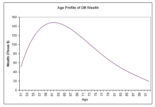
In contrast to the pattern for DCs and IRAs, DB wealth rises about 14 percent from the youngest to the middle cohort, then falls by more than half in the oldest cohort. We can again interpret this in terms of cohort and life-cycle effects. As we discussed above, older households are more likely to be covered by DB plans, so the cohort effect has DB wealth rising with age. The life-cycle effect is nonlinear: the present value of benefits increases rapidly late in working life, but then falls after retirement as life expectancy decreases. Thus for pre-retirees, the cohort and life-cycle effects move in tandem, as seen by the increase in DB wealth between the youngest and middle cohorts. Later in life, however, the life-cycle and cohort effects work in opposite directions: the life-cycle effect calls for lower DB wealth as households age, while the cohort effect offsets this with a tendency toward greater DB wealth among older households, all else equal. We find that the life-cycle effect dominates-there is less DB wealth in the oldest cohort. These patterns are illustrated in the top left panel of Figure 1, which plots the predicted values of a regression of DB wealth on a quartic in age. The figure shows that mean DB wealth nearly triples from $51,000 at age 51 to $148,000 at 62, then gradually declines with age.
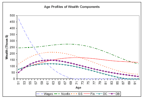
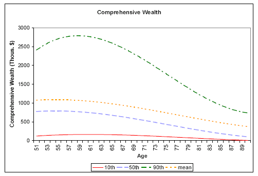
Looking at the evolution of wealth shares with age, Table 2 shows that the share from financial wealth rises steadily, as the shares from Social Security and DC fall.36 These patterns can also be seen in the top right panel of Figure 1, which plots the predicted values of separate regressions of each wealth component on a quartic in age. Financial wealth, the red line, declines only modestly with age, while nonfinancial wealth, Social Security, DB and DC all decline quite steeply. The actuarial present values (e.g., DB and Social Security wealth) decrease mechanically as life expectancies shorten in older age. The bottom left panel of Figure 1 shows that mean comprehensive wealth falls from about $1.1 million at age 51 to $360,000 by age 90. The annuitized value of wealth, however, does not necessarily decline with age, as discussed below.
5.1 Annuity Value of Comprehensive Wealth
Table 3 presents the annuity values of comprehensive wealth by age and lifetime earnings. We use Social Security benefits, which are based on average lifetime earnings, to classify households into low, medium, and high lifetime earnings categories. We begin with annuity values that do not account for household scale economies, as shown in the left-hand panel of Table 3. The figures shown in the first row suggest most households in our sample appear to have sufficient wealth to finance adequate consumption in retirement, in expected value. The overall median annuity value of wealth is about $32,000 per person per year in expected value, and the mean is about $51,000.37 Not all households, however, are as well situated. Households at the 10th percentile can finance just under $9,000 of consumption per expected person-year, which is unlikely to be enough to keep the household out of poverty throughout retirement.38 Even on a per-person basis, couples have significantly larger annuity values than singles, with a median of $36,000 versus $26,000 for singles. The means, however, are much closer.
The right-hand panel of Table 3 shows that, accounting for household economies of scale in consumption, we find a median value of $40,000 of per-person single-equivalent consumption, and a mean of $73,000. Relative to the benchmark case without scale economies, these levels are 26 percent higher at the median and 42 percent at the mean. The effect of accounting for scale economies increases with age and with lifetime earnings. These results help quantify the significant effect of household economies of scale in consumption on the well-being of couples in retirement. However, because the adjustment factor is somewaht arbitrary, we report unadjusted annuity figures throughout the remainder of the paper.
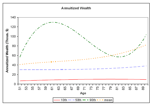
Not surprisingly, Table 3 shows a strong gradient by lifetime earnings, with the median increasing from $17,000 among the low-earning group to $28,000 for the middle group and $47,000 for the high-earning group. This is the pattern we would expect, since households with greater lifetime earnings are able to save more in order to finance greater consumption in retirement. Across ages, the median annuity values of comprehensive wealth are relatively constant, with a slight uptick at older ages. These patterns are shown in more detail in the bottom right panel of Figure 1, which plots the predicted values of regressions on a cubic in age.
A flat age profile of annuitized wealth is what would be predicted by the standard life-cycle model without bequests, in which assets are consumed at exactly the rate required to avoid surpluses or deficits at the end of the expected lifetime. Note that the profiles shown in Figure 1 conflate life-cycle effects, cohort effects, and survivorship effects (i.e., the fact that wealthier households are more likely to live to old ages). Nevertheless, abstracting from cohort and survivorship effects and treating the profile as a true life-cycle effect, we find that the median household is consuming assets at approximately the rate suggested by the life-cycle model. At the mean, there is a positive gradient with age, and at the 90th percentile, we observe a strong peak at about 62, followed by a dip in the mid-80s, followed by another increase at the oldest ages (which could be due to survivorship bias).
There could be three explanations for the positive slope at the mean. First, there could be cohort effects reflecting less saving among the upper quantiles of younger cohorts, relative to the older cohorts. For example, looking at the 90th percentile of annuity values, we see that the first two cohorts are fairly close, at about $85,000 and $95,000, but the third is significantly higher, at $133,000. This could indicate that the upper quantiles of the oldest cohort simply saved more over their lifetime because of relatively high risk aversion or other reasons. Second, there could be survivorship bias: the upper quantiles of the oldest cohort are higher not because they saved more, but because we lack data on the lower-wealth households that died before reaching these ages.
Finally, a third explanation is that the age gradient is neither a cohort effect nor a selection effect, but a true age effect (i.e., the pattern is what would be observed following the average household over time). Under this explanation, the upper-quantile households are under-consuming relative to the Social Security life tables and relative to the standard life cycle model without bequest motives. Recall that the Social Security life tables do not differentiate based on wealth. Thus if higher-wealth households expect to live longer than the life tables imply, they would optimally consume less than the annuity values shown in Table 3. Similarly, if households had bequest motives or precautionary savings motives (e.g., with respect to the risk of large out-of-pocket medical expenses), they would optimally consume less. In either case, consuming less than the annuity value would result in asset growth over time, and thus higher annuity values for older households. Later in the paper we explore some of these possibilities by looking at how the results depend on expectations regarding longevity, medical expenditures, and potential bequests.
5.2 Ratio of Comprehensive Wealth to Poverty-Line Wealth
Next, we formalize the comparison of wealth to poverty by computing the ratio of comprehensive wealth to the actuarial present value of future poverty lines, which we call "poverty-line wealth." Poverty-line wealth varies across households because of differences in household-specific poverty lines, which are functions of the ages and survival probabilities of the household members. Poverty-line wealth can be interpreted as the level of wealth that would be sufficient to finance consumption equal the expected poverty line over the expected remaining lifetimes of the household members.39
Table 4 shows that overall, households hold comprehensive wealth that is several multiples of their poverty-line wealth. The mean ratio is 5.75, and the median is 3.56. The ratios are strongly related to lifetime earnings, but even the lowest earnings group has a median ratio of 1.77. Not all households, however, exceed their poverty-line wealth thresholds. The ratio at the 10th percentile is 0.92, and among the lowest earnings group, the ratio at the 10th percentile is 0.75. The poverty ratios rise slightly with age at the median and relatively steeply at the mean.
Table 5 presents the distribution of poverty ratios in more detail. About 12 percent of households have poverty ratios below one, and another nine percent have a ratio less than 1.5, which we refer to as "near poverty."40 Not surprisingly, there is a close correlation between lifetime earnings and the share of households below or near the poverty line. Close to a third of our sample of households with low lifetime earnings has a ratio of poverty to wealth less than 1.0, and almost 45 percent of this group have a ratio less than 1.5. These shares drop rapidly, however, as we move up the lifetime earnings categories. For instance, only 4 percent of households with middle lifetime earnings have wealth below poverty, with 13 percent near poverty. In the highest-earnings group, there are almost no households at or near poverty. The majority of the highest-earnings households, more than 80 percent, have wealth levels at least three times poverty. Households in the youngest cohort are a bit more likely to be in poverty, a pattern that is consistent with the small positive relationship between age and our wealth measures at the 10th percentile.
Comprehensive Wealth
To explore the sensitivity of our results to the discount-rate assumptions, we recompute the present values with alternative assumptions about real discount rates and inflation. Benefits that are indexed for inflation, such as Social Security and some DB plans, are affected only by changes in the real discount rate, while the other benefits are also affected by changes in inflation. The results, presented in the upper rows of Table 6, show that the effect of alternative assumptions is important for the individual present value calculations, but smaller for the overall comprehensive wealth measure.
For example, lowering the real discount rate from 2.5 percent to 1 percent increases the mean present value of expected Social Security benefits by about $37,000, or 24 percent, while increasing it to 4 percent lowers the mean by about $27,000, or 17 percent. Similarly, lowering the nominal discount rate from 4.5 percent to 2 percent increases the mean present value of expected DB payments by about $27,000, or 26 percent, while increasing the nominal rate to 7 percent reduces the mean by about about $18,000, or 18 percent. The sensitivity of DB wealth to inflation is limited by the relatively high share (about 40 percent) of DB recipients who report inflation-indexed benefits (most often public-sector workers). The resulting percentage changes in comprehensive wealth, however, are only about half as big, since the present value calculations account for just under half of comprehensive wealth.
Annuity Values
Table 6 also shows how the annuity value calculation changes under different assumptions about real interest rates and inflation.41 The different assumptions change the annuity values by about 5 to 10 percent, but this is not enough to affect any of the major patterns or conclusions.
Table 7 provides annuity values for less comprehensive measures of wealth. Since there is some disagreement among researchers about whether housing wealth should be included (see Mitchell and Moore, 1998; Bernheim, 1992), we provide an alternative calculation that excludes nonfinancial wealth. Removing housing and other nonfinancial assets takes about $9,000, or nearly a third, off of the median annuity value of wealth, and $15,000 off of the mean. This adjustment has a larger effect on the annuity values of older households, for whom nonfinancial assets make up a larger share of wealth.
Excluding housing flattens out the age-path of mean annuitized wealth somewhat. Ignoring cohort effects and survivorship bias and treating this pattern as a pure age pattern, this flattening suggests that annuitized wealth excluding housing provides a consumption path that is closer to the flat path predicted by the life-cycle model. Thus, interpreted in the context of the standard life-cycle model, this pattern suggests that the average household appears reluctant to tap equity from its house, intends to leave its house as a bequest, or both.
At the median, removing housing results in a declining age-path of annuitized wealth. Applying the same life-cycle interpretation suggests that for the median household, including housing in wealth provides a consumption path closer to the life-cycle prediction. The implication is that the typical household cannot anticipate bequeathing the full value of its house unless it plans on curtailing consumption expenditures during its remaining years of life. Thus, in the context of the standard life-cycle model, one interpretation of this pattern is that wealthier households intend to leave their houses for their heirs, while the median household intends to consume, rather than bequeath, its nonfinancial wealth.
Table 7 also presents calculations of annuitized wealth excluding both housing and all the present-value calculations. This narrow measure of wealth, which consists only of financial wealth and retirement accounts, is sometimes used to gauge savings adequacy. Table 7 shows that, by this measure, savings is clearly inadequate, with a median annuity value of only $2,300 per person per year. It is doubtful, however, whether households really intend to finance retirement consumption out of financial assets alone. Indeed, because the annuity values of financial wealth rise steeply with age, households would be underconsuming if they were relying solely on financial assets. Thus, in the context of the life-cycle model, it appears that many households are relying on broader sources of wealth (such as pensions, Social Security and housing) to finance retirement consumption.
Poverty Ratios
Table 6 also compares the average poverty ratios calculated with our baseline assumptions (2.5% real interest rate and 2% inflation) with four alternative assumptions that allow for higher and lower values of inflation and interest rates. For a given real interest rate, increasing the inflation rate from 1 percent to 3 percent decreases the poverty ratios by a fairly small amount--about 3 percent. The ratio falls because some of the wealth components in the numerator of the ratio are not indexed to inflation, while the poverty lines in the denominator are fully indexed.
While inflation has only a minor effect on the ratios, the real interest rate plays a larger role. Holding inflation constant, increasing the real interest rate from 1 percent to 4 percent increases the poverty ratios by about 15 percent. The intuition for the relatively large magnitude is that while the numerator contains some non-present-value components (e.g., financial wealth, retirement accounts, and housing), the denominator consists entirely of the discounted streams of future poverty lines, which are quite sensitive to changes in the discount rate. An increase in the real interest rate therefore decreases the present value in the denominator by more than it decreases the values in the numerator, causing a substantial increase in the size of the ratio.
Finally, Table 6 reports the sensitivity to discounting assumptions of the share of households below poverty. Because the poverty line and many components of wealth are unaffected by inflation, the distribution of poverty ratios is relatively insensitive to the level of inflation. The level of real interest rates, however, has a modest impact on the distribution, with fewer households estimated to fall below the poverty threshold when real rates are higher. Since both the numerator and denominator of the poverty ratio are affected by real rates, this result shows that the effect on the denominator (i.e., a lower present value of future poverty lines when real rates are higher) outweighs the effect on the numerator (i.e., a lower present value of future wages, pensions, Social Security, life insurance and welfare).
Table 8 repeats the exercise of analyzing the effect on the results of using narrower measures of wealth. Excluding nonfinancial assets lowers the poverty ratio by 1.25 times poverty wealth at the median, and nearly two times poverty at the mean.42 Further excluding all the present value calculations drops wealth well below the poverty threshold at the median, with a ratio of just 0.26. The mean ratio for this narrow measure of poverty is 1.63.
Alternative Retirement Ages
Table 9 shows the effects of assuming alternative retirement ages (for current workers) to the age 62 used in our baseline case. As shown in the table, workers can increase their retirement assets by delaying retirement. For example, delaying retirement from age 62 to age 65 increases median comprehensive wealth by about $30,500, which increases the median annuity value of wealth by about $2,000 per person per year, or 5-1/2 percent. Under the age-65 assumption, the share of households with less than poverty wealth falls from 11.7 percent to 10.9 percent. These figures illustrate that the results do change with alternative assumptions on the retirement age, but overall the changes are relatively modest.
Effect of an Unexpected Social Security Benefit Cut
Given the uncertain future of Social Security and the important role it plays for many older households, a question of interest is what would be the effect of a cut in Social Security benefits. Since we are not modeling savings decisions in this paper, we will restrict our simulation to unexpected benefit cuts (i.e., we ignore savings responses). In our final sensitivity analysis, we simulate an across-the-board reduction of 25 percent in the present value of benefits among all households in the sample (i.e., including current retirees).
The results are shown in Table 10. The effect of an across-the-board cut on the median household would be to reduce the annuitized value of wealth by about $2,500, or 8 percent. The ratio of wealth to poverty would fall from 3.56 to 3.29, and the share of households under the poverty threshold would go up by about three percentage points. By age, the largest effect is on the middle cohort, and by lifetime earnings, the biggest impact is on those with medium earnings (in part because some of the lowest-earning households have no Social Security benefits at all). For the middle-earning group, the benefit cut reduces annuitized wealth by about 9 percent, and increases the share below poverty from 4 percent to 10 percent.
5.4 Wealth by Poverty Class
Next we explore how sources of wealth differ between poor and non-poor households. Table 11 breaks down the components of wealth for households classified by poverty ratio. Clearly, poverty households--those with wealth-to-poverty ratios less than one--have fewer of all assets (except, in some cases, veterans and welfare benefits). In addition to having negative mean financial assets, they are also less likely to own houses, retirement accounts, DB plans, or life insurance. Overall, the mean comprehensive wealth of poverty households is about $72,000, less than half of that of those near poverty (defined as those with ratios between 1.0 and 1.5), and only about 5 percent of that held by households with ratios of at least 3.0. Wealth shares clearly differ by poverty status, as well. A feature that stands out is the diminishing importance of Social Security for wealthier households. With each higher poverty classification, the share of Social Security declines markedly, from over half among poverty households to about 15 percent in the top group. Another noteworthy trend is that the share due to DB and DC pension assets increases with wealth. While these savings vehicles constitute only a tiny fraction of resources among poverty households, they account for over a fifth of total wealth in the top group. The mean annuity value of wealth for poverty households is about $6,200 per person per year, compared to over $78,900 per person per year for the top wealth group.43
The lower panel of Table 11 shows that poverty households are more likely to be younger, and are dramatically more likely to come from a lifetime of low earnings. Indeed, 86 percent of poverty households have had low lifetime earnings, suggesting that low human capital or significant negative shocks early in life, such as a disabling illness or injury, are the root causes of their poverty in retirement.
5.5 Regression Results
With only a cross-section, it is difficult to identify the importance of factors such as health uncertainty and bequests for the adequacy of savings, since we cannot separate age and cohort effects. Nevertheless, it is informative to examine cross-sectional regression results. Tables 12 and 13 display the coefficient estimates of OLS regressions of annuitized wealth and the poverty ratio on a set of household characteristics. Both sets of results generally move in the same direction, so we will focus on the results pertaining to poverty ratios.
As we would expect from the results in our previous tables, the age of the oldest household member is positively correlated with the mean amount of wealth relative to poverty. The coefficient estimates for our four age groups (61-70, 71-80, 81-90, and 91+) are 0.96, 1.77, 2.69, and 5.23, with the last three significant at the 1% level. The tendency for wealth to rise with age raises the possibility that some households are under-consuming out of their total wealth. As noted earlier, of course, there are other interpretations. One possibility is that the cross-sectional regression is picking up cohort differences in saving parameters such as the coefficient of relative risk aversion and the discount rate. For example, one could point to the Depression generation's historically reinforced fear of losing wealth in the event of an economic crisis as an explanation for their higher-than-average poverty ratios. In contrast, the baby boomers, who have experienced comparatively benign economic events, might be less risk averse and more sanguine about the future. Similarly, younger cohorts may be more willing to conusme out of housing wealth, via downsizing or reverse mortgages.
A second explanation of the rising wealth-to-poverty ratios could be differences in the demographic changes experiences by different cohorts (Gale and Pence, 2006). For instance, older cohorts may have experienced higher-than-expected lifetime earnings relative to younger cohorts and saved more accordingly. Finally, there is the possibility of survivorship bias: if wealthier households are likely to live longer, they may be over-represented in our sample of the oldest households.
The HRS includes some questions that allow us to address the importance of expectations over life cycle variables such as mortality, health status, and bequests. Table 13 reports coefficient estimates for different expectations of health and inheritance. The first question asks about the probability of living about 10 more years. The coefficient estimate for respondents reporting probabilities lower than those in the Social Security life tables is -0.354, while the estimate for respondents reporting higher probabilities is 0.257. Neither is statistically significant at the 10% level, perhaps reflecting the imprecision with which these expectations are measured by this question. Nonetheless, the sign of the result is consistent with both differential mortality (i.e., lower-wealth households correctly expect to die sooner) and the life cycle model (i.e., households that expect to die earlier will tend to draw down their assets more rapidly).
Most of the other variables in Table 13 generate predictions consistent with the life cycle model. Controlling for other factors, the poverty ratios of households strongly expecting to leave large bequests (greater than $100,000) are higher by about 5.361. In contrast, households that expect to receive inheritances tend to have lower poverty ratios, but the relationship is not statistically significant. Households that anticipate having to work past the age of 65 have lower wealth than those that expect to retire by that age, consistent with the idea that households expect to consume less leisure if they arrive at retirement age with fewer resources.
The relationship between a household's expectations about entering a nursing home and its level of wealth is somewhat nonlinear. Households that expect to move into a nursing home with a "medium" probability (defined as between 20% and 80%) appear to have more wealth than those whose with a low probability, a pattern consistent with precautionary saving. However, households with a high probability of entering a nursing home have less wealth. One explanation is that households often face an incentive to run down assets if they anticipate entering a nursing home (Kotlikoff, 1988); another is that rising medical expenses have already weakened their household balance sheet.
5.6 The Effect of Health Status
The optimality of saving decisions can depend crucially on individuals' uncertainty about, and experience of, shocks to health status and medical expenses (Palumbo, 1999; French, 2005; French and Jones, 2004a). It is not immediately clear, however, exactly how the presence of health uncertainty should affect the adequacy of savings. On one hand, households facing either greater health uncertainty or higher predicted medical expenses should accumulate a larger buffer-stock of savings to self-insure against these expected costs. But on the other hand, realizations of medical expense shocks can reduce the existing balance sheets of households. Even households that predicted high future medical expenses would be likely to experience a substantial drop in wealth when these predictions are realized. The limitations of cross-sectional data prevent us from understanding the evolution of savings in the face of health uncertainty, but we can discuss correlations of wealth with various measures of health status and medical costs.
Table 13 shows how our adequacy measures correlate with different measures of health. The HRS includes questions about individuals' self-reported health status. The omitted category in the regression is "excellent/very good." The coefficient estimates decline from -0.535 for "good" health to -1.232 for "fair/poor" health. A similar relationship emerges when we examine other health measures, such as the number of diagnosed conditions or body mass index. At first glance, out-of-pocket medical expenses appears to deviate from this pattern, with larger expenses corresponding to higher levels of wealth adequacy. But this result is probably just picking up the fact that wealthier households can afford larger out-of-pocket expenses such as private nursing homes.
A number of interpretations are consistent with the positive relationship between health status and wealth. First, because current health depends on past health (French and Jones, 2004b), and health is an important determinant of labor earnings, we can expect that many individuals in poor health also experienced relatively low lifetime earnings. Second, to the extent that adverse health outcomes increase out-of-pocket medical expenses, some of the households in poor health may have exhausted a large portion of savings on health expenditures. Third, if health status depends positively on lifetime earnings, as would be the case if preventative and ameliorative health expenses are normal goods, lower lifetime earnings would be associated with worse average health outcomes. Finally, because health status is correlated with expected mortality, the life cycle model predicts that, other factors held constant, households in poor health should dissave more rapidly since they face a shorter decision horizon.
Another way to characterize the relationship between household characteristics and wealth adequacy is to consider the probability of having wealth below poverty. Table 14 displays the coefficient estimates for a linear probability model of a poverty indicator on household characteristics. As in our other regressions, age and lifetime earnings are positively and significantly correlated with our measure of wealth. Households aged 71-80, for instance, are 8 percentage points less likely to be in poverty than those aged 51-60. Health status continues to be an important indicator of poverty. Households who report being in fair to poor health are about 3 percentage points more likely to have wealth below poverty than households who report being in good health.
The composition of assets is strongly related to the probability of being poor. According to the results in Table 14, households who own non-financial assets are almost 30 percentage points less likely to have wealth less than poverty than those without non-financial assets. This accords with our intuition that households without houses or cars are much more likely to be poor. Ownership of retirement assets such as IRAs, DBs, and DCs is worth 5 to 8 percentage points less probability of poverty, and Social Security is worth even more, about 11 percentage points. Since we our using Social Security as a proxy for lifetime earnings, the probability model is picking up two effects. First, lower lifetime earnings (expected Social Security payments) increase the probability a household will have wealth below poverty. Second, households with no expected Social Security benefits are even more likely to have inadequate wealth since these households are at the very bottom of the lifetime earnings distribution.
6 Conclusion
The retiring baby boomers, the prospect of Social Security and Medicare reforms, and the transition from traditional pensions to retirement accounts have focused policy makers' attention on the current and projected adequacy of retirement wealth in the U.S. Our study joins several others in an attempt to answer some fundamental questions about adequacy: How much wealth is enough? How many households have it? And, what is the distribution of resources?
We approached the first question by constructing two measures of adequacy based on a comprehensive measure of wealth that includes the expected present value of Social Security, defined benefit pensions, life insurance, annuities, welfare payments, and future labor earnings. Annuitized comprehensive wealth tells us the amount of consumption a household can expect to finance per person per year over their remaining lifetimes. The ratio of comprehensive wealth to the expected present value of future poverty lines provides a notion of absolute adequacy that is built on a widely used framework for analyzing poverty in the U.S.
Consistent with the somewhat optimistic results in some of the previous studies,44 we find that, by our measures, most households over age 50 can expect to have adequate resources throughout retirement. We find a mean comprehensive wealth of about $900,000, and a median of about $536,000. Abstracting from household scale economies, we find an average annuity value of about $51,000 per expected person-year, with a median of $32,000. Accounting for economies of scale, we find to $73,000 of single-equivalent consumption per person at the mean, and $40,000 at the median.
Our analysis indicates that most households have comprehensive wealth well above the levels needed to finance poverty-line consumption: the mean ratio of wealth to the present value of future poverty lines is 5.75, and the median is 3.56. However, we see problems in the left tail--the ratio at the 10th percentile is 0.92. Overall, we find that about 12 percent of households fall below poverty-line wealth, and an additional nine percent are close to poverty (with ratios between 1.0 and 1.5).
With regard to some of the trends that motivated our analysis, we conclude that, by our measures, the early wave of the baby boom generation appears to be on track to accumulating adequate retirement wealth. We find a median annuitized value wealth equal to $30,000 per person and a mean of $47,000, with a median ratio of wealth to the present value of poverty lines of 3.35. However, we find that about 27 percent of the early baby-boom cohort's comprehensive wealth is held in the form of expected future wages, and that the financial assets of this cohort is significantly lower than that of older cohorts. This is not entirely surprising, since this cohort was still in its peak earnings and savings years in 2004. But it emphasizes the point that, because the baby boomers are still in their working years, their consumption in retirement will depend crucially on their saving and labor-supply behavior and wage growth over their remaining years of work.
Finally, we find evidence suggesting significant cohort effects resulting from the transition from DB to DC pension plans. The share of 51-61 year-olds with DB wealth is about 30 percent, compared to about 44 percent for older households. On the other hand, 61 percent of 51-61 year-olds hold retirement accounts, compared with half of 62-75 year-olds and less than a third of households over 75 (though of course this pattern includes life-cycle effects as well as cohort effects). Despite these changes to pension coverage, however, we do not find evidence of a steep deterioration in retirement adequacy among the younger households in our sample.
Overall, our findings show a generally optimistic view of retirement savings adequacy among current older cohorts, though with a notable pocket of inadequacy concentrated among those with the lowest lifetime earnings. However, we should note several caveats about our results. First, our measures of adequacy are based on expected values, and thus do not account for the substantial risks that arise from uncertain lifetimes, medical expenses and asset returns. Thus a risk-averse household with "adequate" wealth by our measures may not have enough wealth after accounting for the effect of these risks on utility. Second, our analysis focuses on households aged 51 and older in 2004, which includes the leading edge of baby boomers, but not younger boomers or succeeding generations. Thus our findings do not provide evidence about the adequacy of retirement savings among younger workers. Finally, our results should not be taken to imply that current household savings are necessarily sufficient in the long-run macroeconomic sense. The broad demographic trends at work over the next half century, including declining fertility and increasing longevity, imply that a higher household savings rate could, by increasing the size of the capital stock, significantly reduce the burden of higher taxes or lower spending that will otherwise fall on following generations. Viewed in this context, our findings are encouraging, to the extent that they show wealth accumulations at least do not appear to be declining among older households, but they do not show that household saving behavior is optimal in the intergenerational sense.
Data Source
Our primary data sources are the RAND HRS Data File and the 2004 RAND-Enhanced Fat Files. These are HRS data files that have been compiled by RAND, and are often easier to use than the raw HRS data files. The RAND HRS Data File is a longitudinal file in which selected variables have been linked across the seven waves of the HRS. This file includes RAND-generated imputations of missing values. Many variables necessary for our analysis, including detailed DB and DC pension information, are not included in the RAND HRS Data File. For these variables, we use the 2004 RAND-Enhanced Fat File, which includes virtually all the raw HRS data.
A number of income and wealth variables from the 2004 RAND-Enhanced Fat File are missing for some households, but the HRS design includes "unfolding brackets" that provide ranges of values for many of the variables that are missing. We use the brackets to assign imputed values for households who indicate that they have a certain type of income or asset, but do not report the actual amount. If we have information indicating that a respondent should have a value for a particular variable but no information on a range for that value then we assign the missing value a zero. Otherwise, we use the range given by the HRS to impute missing values. Our goal is to match the distribution of imputed values to the distribution of actual values given by respondents.
In order to accomplish this goal, we first find the distribution of actual responses that fall into a given bracket. If there are no actual responses in a specific bracket, the missing value is assigned a zero. If there are, the distribution of actual values in a bracket is divided into ten deciles. Each imputee is randomly assigned a number between one and ten to impute the decile within the self-reported range. Finally, the missing value is replaced with a value that is one-third the distance between the start of the decile and the end of the decile. We use one-third because we find that the central tendency of the empirical distribution of many variables within a given range is often closer to a third than a half.
For example, if we know that a missing variable is between $5,000 and $10,000, we start with the sample of non-missing data between $5,000 and $10,000 and divide this sample into ten deciles, where the decile breaks are not necessarily evenly spaced but rather determined by the empirical distribution. We then randomly assign an imputee to one of the deciles (e.g., the seventh), and give them the value that is one-third of the way through the selected decile.
Note that variables taken from the RAND HRS Data File are imputed by RAND using a different methodology. RAND uses a model-based imputation method and imputes more values than we do. However, we have compared the RAND imputation distribution to our imputation distribution for several variables and can not find any significant differences. For more specific information on the RAND imputation method, please refer to their documentation.
In all calculations, we use the preliminary 2004 weights provided by the HRS.
Present Value Calculations
This section provides a more detailed description of our present value methodology than is found in the main text. We discuss our present value calculations for DB plans, Social Security, annuities, life insurance, and welfare.
Defined Benefit Pensions
Calculating the actuarial present value of future DB pension payments requires a few assumptions. The HRS includes questions about both current pension benefits (for retirees) and expected future pension benefits (for those still working). Households are asked about the (current or expected) pension amount (and start date, if they have not yet begun), cost-of-living adjustments (COLAs), and survivors' benefits.45 In the case of working households, we use the expected pension at retirement; this serves to include the value of benefits not yet accrued. This is parallel to our inclusion of expected future compensation in our calculation of comprehensive wealth.
We express the actuarial present value of DB payments for a plan that pays an annual amount ![]() as
as
![\displaystyle DBPV=d\sum_{\tau=a_{r}}^{119}\delta^{\tau-a_{r}}\bigl\lbrace\psi^{r}(\tau,a_{r})+\theta[1-\psi^{r}(\tau,a_{r})]\psi^{s}(\tau+\Delta,a_{s})\bigr\rbrace,](img22.gif)
where
The conditional survival probabilities are based on the one-year age- and sex-specific conditional death probabilities in the Social Security Administration's 2002 Period Life Table (SSA, 2006c). Period life tables provide a snapshot of the mortality conditions prevailing in a single year, rather than the expected mortality experience of a given cohort over time. For young cohorts (e.g., children born in 2002), one might expect actual longevity to be significantly greater than shown in the 2002 period life table, since longevity generally improves over time. However, since our sample is of Americans aged 51 and older in 2004, we conclude that the 2002 period table (the most recent available) is a reasonable estimate of our sample's expected mortality experience.48
For DB plans with COLAs (about 40 percent of the reported plans), we use a discount factor ![]() equal to
equal to ![]() , where
, where ![]() is the real interest rate. For plans without COLAs, we set
is the real interest rate. For plans without COLAs, we set ![]() equal to
equal to ![]() , where
, where ![]() is the nominal
interest rate. The baseline results in the paper assume a nominal interest rate of 4.5 percent and a real interest rate of 2.5 percent, implying 2 percent inflation. The present value measures are naturally sensitive to the value of
is the nominal
interest rate. The baseline results in the paper assume a nominal interest rate of 4.5 percent and a real interest rate of 2.5 percent, implying 2 percent inflation. The present value measures are naturally sensitive to the value of ![]() , so as a robustness check, we also report results using different assumptions about real rates and inflation.
, so as a robustness check, we also report results using different assumptions about real rates and inflation.
The HRS collects information on multiple pension plans for respondents and their spouses. Applying equation (A-1), we compute present values for each of these and then sum them to arrive at our final calculation for current pensions. Some current workers report that they expect to receive lump-sum payouts from their DB plans upon retirement. To include these plans, we simply discount the lump sum back to the current age:
 |
(A-2) |
where
Social Security
Computing the present value of of Social Security is quite similar to calculating DB wealth. The HRS includes questions about both current benefits for retirees and expected benefits for workers. Let
![]() and
and
![]() denote the current or expected annual social security benefits of the respondent and the spouse at ages
denote the current or expected annual social security benefits of the respondent and the spouse at ages ![]() and
and
![]() respectively. The actuarial present value of household Social Security benefits is given by
respectively. The actuarial present value of household Social Security benefits is given by
![\displaystyle SSPV=\sum_{\tau=a_{r}}^{119}\delta^{\tau-a_{r}}\left[\Psi_{1}(ss^{r}_{\tau}+ss^{s}_{\tau+\Delta})+\Psi_{2}\max(ss^{r}_{\tau},ss^{s}_{\tau+\Delta})\right],](img38.gif)
where
is the conditional probability of both household members being alive, and
is the conditional probability of exactly one household member being alive.49 The first bracketed term in equation (A-3) captures the fact that if both household members are alive, their total benefits will generally equal the sum of their individual amounts. The second term in the brackets reflects the rules governing survivors benefits, whereby a retirement-age widow or widower typically receives 100% of the spouse's benefits if these exceed their own benefit amount.50 Since Social Security benefits are adjusted for inflation, we discount using the real interest rate:
Respondents in the HRS are asked directly about the amount of current or expected spousal benefits. We take these amount at face value and assume that the reported benefits already reflect any adjustments due to the Social Security rules (e.g., the fact that individuals are typically entitled to the maximum of their own benefits and 50% of their spouse's).
Insurance, Annuities, and Welfare
Life insurance policies, annuities, and future welfare payments can constitute an important portion of household wealth. Life insurance wealth is a bit different from DB or Social Security wealth because life insurance is a contingent asset and therefore less liquid than other wealth components. Nonetheless, to ignore it would be to understate the total resources available to finance household consumption in retirement. We only include policies in which the spouse is named as a primary beneficiary.
We compute the actuarial present value of household life insurance as follows:
![\begin{displaymath}\begin{split}INPV={}& \sum_{\tau=a_{r}+1}^{119}\delta^{\tau-a_{r}}\bigl\lbrace\psi^{r}(\tau-1,a_{r})[1-\psi^{r}(\tau,a_{r})]\psi^{s}(\tau+\Delta,a_{s})FV_{r}-\psi^{r}(\tau,a_{r})P_{r} {}& + \psi^{s}(\tau+\Delta-1,a_{s})[1-\psi^{s}(\tau+\Delta,a_{s})]\psi^{r}(\tau,a_{r})FV_{s}-\psi^{s}(\tau+\Delta,a_{s})P_{s}\bigr\rbrace, \end{split}\end{displaymath}](img44.gif)
where
Note that the actuarial present value of insurance would be zero if premiums were actuarially fair and perfectly observed in the data. However, the calculation of life insurance wealth is constrained by data limitations. We do not observe in the HRS the length of term policies, or their premiums.51 In the absence of any data, we assume that term policies will remain in force throughout retirement, and that their premiums have been pre-paid (i.e., are zero in each year going forward). Thus, the only premiums that we account for are those associated with whole life policies. In addition, the HRS does not collect information on the cash value of whole life policies. As a result, we treat term life insurance and whole-life insurance identically in this calculation. That is, we ignore the cash value of whole life policies and instead calculate the present expected value of the face value, regardless of the type of policy.52
Our calculations of wealth from annuities and welfare payments are more straightforward. The formula for calculating the actuarial present value of annuities (![]() ) exactly parallels
equation (A-1), where we make similar adjustments for COLAs and survivor benefits. Our measure of expected welfare payments includes veteran's benefits, food stamps, Supplemental Security Income (SSI), and other welfare. In this calculation, we assume that individuals who are
currently receiving these payments will continue to receive the same inflation-indexed welfare payments as long as they live, and that those not currently receiving these payments never will--i.e., we do not model transitions in and out of welfare-receipt status. Since welfare benefits are
typically indexed to inflation, we discount this stream of expected welfare payments using the real interest rate and the relevant conditional survival probabilities.
) exactly parallels
equation (A-1), where we make similar adjustments for COLAs and survivor benefits. Our measure of expected welfare payments includes veteran's benefits, food stamps, Supplemental Security Income (SSI), and other welfare. In this calculation, we assume that individuals who are
currently receiving these payments will continue to receive the same inflation-indexed welfare payments as long as they live, and that those not currently receiving these payments never will--i.e., we do not model transitions in and out of welfare-receipt status. Since welfare benefits are
typically indexed to inflation, we discount this stream of expected welfare payments using the real interest rate and the relevant conditional survival probabilities.
A2: Annuity Factor Derivation
This section of the appendix derives the annuity factor given by equation (2). We begin by assuming that a respondent (indexed by ![]() ) and a spouse (indexed by
) and a spouse (indexed by
![]() ) want to convert their comprehensive wealth into annuities to finance the same amount of consumption
) want to convert their comprehensive wealth into annuities to finance the same amount of consumption ![]() per person per year. Let
per person per year. Let ![]() be the value of household wealth. Assume that the respondent expects to live
be the value of household wealth. Assume that the respondent expects to live ![]() more years, and the spouse expects to live
more years, and the spouse expects to live ![]() more years. Without loss of generality, we can assume that
more years. Without loss of generality, we can assume that
![]() . Finally, let
. Finally, let
![]() be the nominal discount factor.
be the nominal discount factor.
For the first ![]() years, each member of the household expects to consume
years, each member of the household expects to consume ![]() per
year. The present value of the first
per
year. The present value of the first ![]() years of the household annuities is given by
years of the household annuities is given by
 |
where the last step applies the formula for finite sums. After the respondent dies, the spouse consumes
 |
The sum of these two streams of payments is therefore
 |
We can rewrite this as
![\displaystyle \frac{C\delta}{1-\delta}\left[2-\delta^{T_{r}}-\delta^{T_{s}}\right] = \frac{C}{i}\left[2-\delta^{T_{r}}-\delta^{T_{s}}\right].](img65.gif) |
If the household converts all of its wealth
![\displaystyle CW= \frac{C}{i}\left[2-\delta^{T_{r}}-\delta^{T_{s}}\right],](img66.gif) |
or
where
 |
| Statistics | Exp. PV of Wages thru 61 (1) |
Financial Wealth (2) |
Houses, RE, Veh. & Bus. (3) |
DCs & IRAs (4) |
Exp. PV of DB Plans (5) |
Exp. PV of Soc. Sec. (6) |
Exp. PV of Annuities & Life Ins. (7) |
Exp. PV of Vet. Ben. & Welfare (8) |
Grand Total: Comprehensive Wealth (9) |
|---|---|---|---|---|---|---|---|---|---|
| 10th pctile | 0.0 | -3.0 | 0.1 | 0.0 | 0.0 | 0.0 | 0.0 | 0.0 | 106.7 |
| 50th pctile | 0.0 | 10.5 | 100.5 | 0.1 | 0.0 | 131.6 | 0.0 | 0.0 | 536.6 |
| 90th pctile | 460.0 | 289.0 | 500.0 | 216.0 | 300.0 | 343.3 | 56.9 | 16.3 | 1880.0 |
| Mean | 131.4 | 135.1 | 246.3 | 87.2 | 103.4 | 158.9 | 23.0 | 14.0 | 899.5 |
| Std. Dev. | 344.3 | 1244.6 | 775.8 | 534.9 | 396.8 | 126.8 | 217.7 | 62.8 | 1834.5 |
| Pct with asset | 31.3 | 90.5 | 91.0 | 50.1 | 38.2 | 86.7 | 38.1 | 13.1 | 99.7 |
| Share of Total* | 0.15 | 0.15 | 0.27 | 0.10 | 0.12 | 0.18 | 0.03 | 0.02 | 1.00 |
| Gini | 0.84 | 0.89 | 0.71 | 0.85 | 0.85 | 0.44 | 0.89 | 0.95 | 0.56 |
| Cumulative Gini | 0.84 | 0.77 | 0.67 | 0.67 | 0.64 | 0.57 | 0.57 | 0.56 | 0.56 |
| Statistics | Exp. PV of Wages thru 61 (1) |
Financial Wealth (2) |
Houses, RE, Veh. & Bus. (3) |
DCs & IRAs (4) |
Exp. PV of DB Plans (5) |
Exp. PV of Soc. Sec. (6) |
Exp. PV of Annuities & Life Ins. (7) |
Exp. PV of Vet. Ben. & Welfare (8) |
Grand Total: Comprehensive Wealth (9) |
|---|---|---|---|---|---|---|---|---|---|
| 10th pctile | 68.2 | -4.0 | 7.0 | 6.0 | 18.8 | 56.4 | 2.6 | 2.3 | 108.4 |
| 50th pctile | 285.1 | 18.0 | 120.0 | 60.0 | 129.4 | 154.9 | 23.6 | 49.7 | 538.8 |
| 90th pctile | 859.3 | 320.0 | 532.0 | 400.0 | 613.0 | 355.6 | 125.3 | 271.9 | 1882.8 |
| Mean | 419.8 | 149.3 | 270.8 | 173.9 | 270.9 | 183.4 | 60.4 | 107.4 | 901.9 |
| Std. Dev. | 507.7 | 1307.4 | 809.4 | 745.4 | 605.8 | 118.6 | 349.3 | 142.0 | 1836.4 |
| Share of Total* | 0.34 | 0.15 | 0.28 | 0.13 | 0.25 | 0.20 | 0.04 | 0.08 | 1.00 |
| Gini | 0.49 | 0.88 | 0.68 | 0.70 | 0.62 | 0.36 | 0.70 | 0.61 | 0.57 |
- *Share is calculated as ratio of means, rather than mean of ratios.
- Source: Authors' calculations from the RAND HRS Data File and the 2004 RAND-Enhanced Fat Files. Sample size = 12,861 households.
| Statistics | Exp. PV of Wages thru 61 (1) |
Financial Wealth (2) |
Houses, RE, Veh. & Bus. (3) |
DCs & IRAs (4) |
Exp. PV of DB Plans (5) |
Exp. PV of Soc. Sec. (6) |
Exp. PV of Annuities & Life Ins. (7) |
Exp. PV of Vet. Ben. & Welfare (8) |
Grand Total: Comprehensive Wealth (9) |
|---|---|---|---|---|---|---|---|---|---|
| 10th pctile | 0.0 | -8.0 | 1.0 | 0.0 | 0.0 | 0.0 | 0.0 | 0.0 | 139.3 |
| 50th pctile | 141.8 | 6.0 | 96.0 | 12.0 | 0.0 | 151.8 | 0.0 | 0.0 | 724.2 |
| 90th pctile | 731.5 | 225.2 | 486.6 | 270.0 | 356.6 | 353.4 | 79.3 | 24.0 | 2211.6 |
| Mean | 286.1 | 91.5 | 247.3 | 102.9 | 110.6 | 167.6 | 27.0 | 18.1 | 1051.2 |
| Std. | 471.3 | 374.3 | 755.2 | 399.5 | 347.8 | 130.9 | 80.3 | 76.6 | 1309.4 |
| Pct with asset | 64.8 | 90.0 | 93.2 | 61.3 | 30.3 | 82.7 | 42.4 | 12.0 | 99.5 |
| Share of Total* | 0.27 | 0.09 | 0.23 | 0.10 | 0.11 | 0.16 | 0.03 | 0.02 | 1.00 |
| Gini | 0.66 | 0.94 | 0.72 | 0.81 | 0.87 | 0.44 | 0.84 | 0.95 | 0.51 |
| Cumulative Gini | 0.66 | 0.64 | 0.60 | 0.60 | 0.58 | 0.52 | 0.52 | 0.51 | 0.51 |
| Statistics | Exp. PV of Wages thru 61 (1) |
Financial Wealth (2) |
Houses, RE, Veh. & Bus. (3) |
DCs & IRAs (4) |
Exp. PV of DB Plans (5) |
Exp. PV of Soc. Sec. (6) |
Exp. PV of Annuities & Life Ins. (7) |
Exp. PV of Vet. Ben. & Welfare (8) |
Grand Total: Comprehensive Wealth (9) |
|---|---|---|---|---|---|---|---|---|---|
| 10th pctile | 0.0 | -2.0 | 1.0 | 0.0 | 0.0 | 16.3 | 0.0 | 0.0 | 123.2 |
| 50th pctile | 0.0 | 14.2 | 115.0 | 0.2 | 0.0 | 170.5 | 0.0 | 0.0 | 537.6 |
| 90th pctile | 0.0 | 301.3 | 550.0 | 240.0 | 369.1 | 381.7 | 50.0 | 17.1 | 1816.6 |
| Mean | 19.5 | 177.8 | 281.8 | 106.0 | 126.5 | 194.4 | 19.3 | 14.0 | 939.4 |
| Std. | 96.1 | 1989.5 | 946.7 | 798.5 | 429.7 | 132.7 | 74.8 | 59.9 | 2570.6 |
| Pct with asset | 9.0 | 91.1 | 92.6 | 50.3 | 43.9 | 90.7 | 40.5 | 13.7 | 99.9 |
| Share of Total* | 0.02 | 0.19 | 0.30 | 0.11 | 0.13 | 0.21 | 0.02 | 0.01 | 1.00 |
| Gini | 0.96 | 0.90 | 0.71 | 0.86 | 0.81 | 0.38 | 0.88 | 0.95 | 0.57 |
| Cumulative Gini | 0.96 | 0.87 | 0.73 | 0.73 | 0.68 | 0.58 | 0.58 | 0.57 | 0.57 |
| Statistics | Exp. PV of Wages thru 61 (1) |
Financial Wealth (2) |
Houses, RE, Veh. & Bus. (3) |
DCs & IRAs (4) |
Exp. PV of DB Plans (5) |
Exp. PV of Soc. Sec. (6) |
Exp. PV of Annuities & Life Ins. (7) |
Exp. PV of Vet. Ben. & Welfare (8) |
Grand Total: Comprehensive Wealth (9) |
|---|---|---|---|---|---|---|---|---|---|
| 10th pctile | 0.0 | 0.0 | 0.0 | 0.0 | 0.0 | 0.0 | 0.0 | 0.0 | 67.2 |
| 50th pctile | 0.0 | 22.6 | 91.0 | 0.0 | 0.0 | 78.1 | 0.0 | 0.0 | 292.5 |
| 90th pctile | 0.0 | 400.0 | 441.0 | 80.0 | 123.9 | 187.7 | 17.9 | 9.0 | 1177.6 |
| Mean | 0.5 | 155.9 | 193.0 | 30.2 | 56.5 | 91.1 | 20.9 | 6.4 | 554.4 |
| Std. | 9.9 | 851.9 | 481.0 | 114.2 | 429.1 | 72.8 | 430.6 | 27.0 | 1279.3 |
| Pct with asset | 0.3 | 90.7 | 84.4 | 28.8 | 43.3 | 88.5 | 26.8 | 14.2 | 99.7 |
| Share of Total* | 0.0 | 0.28 | 0.35 | 0.05 | 0.10 | 0.16 | 0.04 | 0.01 | 1.00 |
| Gini | 1.00 | 0.82 | 0.68 | 0.90 | 0.86 | 0.42 | 0.96 | 0.94 | 0.58 |
| Cumulative Gini | 1.00 | 0.82 | 0.68 | 0.68 | 0.66 | 0.58 | 0.59 | 0.58 | 0.58 |
- *Share is calculated as ratio of means, rather than mean of ratios.
- Source: Authors' calculations from the RAND HRS Data File and the 2004 RAND-Enhanced Fat Files. Sample size = 12,861 households.
| Lifetime Earnings |
Without Scale Economies: 10th Percentile | Without Scale Economies: 50th Percentile | Without Scale Economies: 90th Percentile | Without Scale Economies: Mean | With Scale Economies: 10th Percentile | With Scale Economies: 50th Percentile | With Scale Economies: 90th Percentile | With Scale Economies: Mean |
|---|---|---|---|---|---|---|---|---|
| All | 9.1 | 31.5 | 96.1 | 51.2 | 9.8 | 39.6 | 129.2 | 72.6 |
| Single | 7.8 | 26.0 | 98.1 | 50.3 | 7.8 | 26.0 | 98.1 | 50.3 |
| Married | 12.2 | 35.9 | 95.2 | 52.1 | 17.6 | 52.4 | 149.1 | 94.4 |
| Low | 4.7 | 17.0 | 76.2 | 37.4 | 5.1 | 19.4 | 96.3 | 53.2 |
| Middle | 12.0 | 28.4 | 81.2 | 43.0 | 13.2 | 35.3 | 111.3 | 58.5 |
| High | 20.4 | 47.2 | 120.1 | 72.9 | 25.7 | 60.4 | 163.4 | 105.7 |
| Lifetime Earnings |
Without Scale Economies: 10th Percentile | Without Scale Economies: 50th Percentile | Without Scale Economies: 90th Percentile | Without Scale Economies: Mean | With Scale Economies: 10th Percentile | With Scale Economies: 50th Percentile | With Scale Economies: 90th Percentile | With Scale Economies: Mean |
|---|---|---|---|---|---|---|---|---|
| All | 7.8 | 30.3 | 84.7 | 42.7 | 5.2 | 37.1 | 102.8 | 51.6 |
| Low | 3.4 | 15.6 | 66.2 | 29.3 | 4.0 | 17.3 | 77.1 | 33.7 |
| Middle | 10.8 | 25.9 | 65.8 | 35.9 | 11.7 | 32.0 | 76.4 | 43.1 |
| High | 19.9 | 44.0 | 101.5 | 58.1 | 24.4 | 54.6 | 128.9 | 72.0 |
| Lifetime Earnings |
Without Scale Economies: 10th Percentile | Without Scale Economies: 50th Percentile | Without Scale Economies: 90th Percentile | Without Scale Economies: Mean | With Scale Economies: 10th Percentile | With Scale Economies: 50th Percentile | With Scale Economies: 90th Percentile | With Scale Economies: Mean |
|---|---|---|---|---|---|---|---|---|
| All | 9.6 | 30.9 | 94.7 | 52.5 | 10.7 | 40.0 | 124.9 | 67.1 |
| Low | 5.5 | 16.3 | 74.0 | 39.6 | 5.9 | 18.9 | 93.7 | 48.0 |
| Middle | 12.5 | 26.9 | 75.5 | 39.2 | 13.5 | 33.2 | 98.1 | 49.8 |
| High | 21.1 | 48.3 | 124.9 | 79.3 | 27.5 | 63.0 | 167.3 | 104.1 |
| Lifetime Earnings |
Without Scale Economies: 10th Percentile | Without Scale Economies: 50th Percentile | Without Scale Economies: 90th Percentile | With Scale Economies: Mean | With Scale Economies: 10th Percentile | With Scale Economies: 50th Percentile | With Scale Economies: 90th Percentile | With Scale Economies: Mean |
|---|---|---|---|---|---|---|---|---|
| All | 10.1 | 34.6 | 132.9 | 65.4 | 11.0 | 45.7 | 194.6 | 120.2 |
| Low | 7.0 | 21.5 | 115.0 | 50.9 | 7.4 | 27.1 | 149.5 | 99.8 |
| Middle | 13.1 | 33.4 | 112.4 | 54.4 | 13.8 | 44.1 | 162.5 | 83.9 |
| High | 22.5 | 62.2 | 191.1 | 114.3 | 26.7 | 88.0 | 352.6 | 237.8 |
- Note: Comprehensive wealth per expected person-year, in thousands of 2004 dollars. Scale economies reflect an assumption that married couples can enjoy an equivalent amount of per-capita consumption as singles by spending 1.66 times the singles' expenditure (vs. a baseline of 2 times). Lifetime earnings grouped by position in distribution of Social Security benefits. See text for details. Sample size = 12,861 households.
| Age: Lifetime Earnings | 10th Percentile | 50th Percentile | 90th Percentile | Mean |
|---|---|---|---|---|
| All (51+): All | 0.92 | 3.56 | 11.11 | 5.75 |
| All (51+): Single | 0.73 | 2.47 | 9.39 | 4.84 |
| All (51+): Married | 1.55 | 4.56 | 12.11 | 6.64 |
| All (51+): Low | 0.47 | 1.77 | 8.44 | 4.02 |
| All (51+): Middle | 1.26 | 3.19 | 9.45 | 4.81 |
| All (51+): High | 2.34 | 5.44 | 14.24 | 8.39 |
| 51-61: All | 0.75 | 3.35 | 9.38 | 4.67 |
| 51-61: Low | 0.34 | 1.54 | 7.07 | 3.00 |
| 51-61: Middle | 1.06 | 2.92 | 6.99 | 3.90 |
| 51-61: High | 2.21 | 4.99 | 11.85 | 6.55 |
| 62-75: All | 1.01 | 3.65 | 11.22 | 6.12 |
| 62-75: Low | 0.58 | 1.77 | 8.55 | 4.42 |
| 62-75: Middle | 1.30 | 3.07 | 8.73 | 4.52 |
| 62-75: High | 2.57 | 5.77 | 14.89 | 9.47 |
| 1.08 | 3.91 | 14.66 | 7.26 | |
| 0.73 | 2.35 | 12.17 | 5.57 | |
| 1.36 | 3.84 | 12.25 | 6.04 | |
| 2.58 | 6.95 | 22.63 | 12.82 |
- Note: Ratio of comprehensive household wealth to expected present value of the household-specific poverty line. Lifetime earnings grouped by position in distribution of Social Security benefits. See text for details. Sample size = 12,861 households.
| Age: Lifetime Earnings |
1.0-1.5 | 1.5-3.0 | ||
|---|---|---|---|---|
| All (51+): All | 12 | 9 | 23 | 57 |
| All (51+): Single | 19 | 14 | 25 | 43 |
| All (51+): Married | 5 | 5 | 20 | 70 |
| All (51+): Low | 31 | 13 | 20 | 35 |
| All (51+): Middle | 4 | 13 | 30 | 53 |
| All (51+): High | 1 | 2 | 17 | 81 |
| 51-61: All | 15 | 9 | 22 | 54 |
| 51-61: Low | 35 | 14 | 19 | 32 |
| 51-61: Middle | 9 | 13 | 30 | 48 |
| 51-61: High | 1 | 3 | 19 | 78 |
| 62-75: All | 10 | 9 | 23 | 58 |
| 62-75: Low | 31 | 14 | 21 | 34 |
| 62-75: Middle | 2 | 13 | 33 | 51 |
| 62-75: High | 0 | 1 | 14 | 85 |
| 8 | 9 | 23 | 59 | |
| 24 | 11 | 22 | 43 | |
| 2 | 11 | 27 | 60 | |
| 0 | 0 | 16 | 84 |
- Note: Poverty ratio is ratio of comprehensive household wealth to expected present value of the household-specific poverty line. Lifetime earnings grouped by position in distribution of Social Security benefits. See text for details. Sample size = 12,861 households.
| Statistic | |||||
|---|---|---|---|---|---|
| PV of Wages | 140.3 | 123.6 | 140.3 | 123.6 | 131.4 |
| PV of DB | 130.4 | 94.7 | 114.2 | 85.3 | 103.4 |
| PV of SS | 196.3 | 131.6 | 196.3 | 131.6 | 158.9 |
| PV of Annuities & LI | 30.9 | 21.8 | 24.3 | 18.0 | 23.0 |
| PV of Vet. & Welfare | 16.5 | 12.2 | 16.5 | 12.2 | 14.0 |
| Comprehensive Wealth | 983.1 | 852.6 | 960.2 | 839.4 | 899.5 |
| Annuitized Wealth | 44.9 | 50.9 | 51.9 | 57.9 | 51.2 |
| Poverty Ratio | 5.36 | 6.24 | 5.26 | 6.17 | 5.75 |
| Share Below Poverty | 12 | 11 | 12 | 11 | 12 |
- Note: Thousands of 2004 dollars. Sample size = 12,861 households.
| Cohort | Comprehensive Wealth Med. |
Comprehensive Wealth Mean |
Ex. Nonfinancial Wealth Med. |
Ex. Nonfinancial Wealth Mean |
Ex. Nonfinancial & PV Wealth Med. |
Ex. Nonfinancial & PV Wealth Mean |
|---|---|---|---|---|---|---|
| All | 31.5 | 51.2 | 22.2 | 36.1 | 2.3 | 14.5 |
| 51-61 | 30.3 | 42.7 | 23.8 | 32.6 | 1.7 | 8.4 |
| 62-75 | 30.9 | 52.5 | 21.2 | 36.4 | 2.5 | 16.3 |
| 34.6 | 65.4 | 20.6 | 42.3 | 4.1 | 23.4 | |
| Owns House | 38.5 | 59.2 | 25.8 | 40.3 | 3.6 | 16.9 |
| No House | 13.3 | 22.1 | 12.9 | 20.9 | 0.1 | 6.1 |
- Note: Thousands of 2004 dollars. Sample size = 12,861 households. About 78 percent of the sample owns a house.
| Cohort | Comprehensive Wealth Med. |
Comprehensive Wealth Mean |
Ex. Nonfinancial Wealth Med. |
Ex. Nonfinancial Wealth Mean |
Ex. Nonfinancial & PV Wealth Med. |
Ex. Nonfinancial & PV Wealth Mean |
|---|---|---|---|---|---|---|
| All | 4.08 | 6.53 | 2.84 | 4.62 | 0.26 | 1.63 |
| 51-61 | 3.99 | 5.56 | 3.08 | 4.25 | 0.19 | 0.91 |
| 62-75 | 4.13 | 6.94 | 2.81 | 4.82 | 0.29 | 1.90 |
| 4.21 | 7.77 | 2.48 | 5.04 | 0.47 | 2.58 | |
| Owns House | 4.36 | 6.72 | 2.97 | 4.58 | 0.42 | 1.90 |
| No House | 1.33 | 2.27 | 1.29 | 2.15 | 0.01 | 0.64 |
- Note: Sample size = 12,861 households. About 78 percent of the sample owns a house.
| Statistic | 60 | 61 | 62 | 63 | 64 | 65 |
|---|---|---|---|---|---|---|
| Comprehensive Wealth median | 516.3 | 524.8 | 536.6 | 545.9 | 555.7 | 566.7 |
| Comprehensive Wealth mean | 868.5 | 883.5 | 899.5 | 914.8 | 930.6 | 946.3 |
| Annuitized Wealth* median | 30.1 | 30.8 | 31.5 | 32.1 | 32.8 | 33.4 |
| Annuitized Wealth* mean | 49.9 | 50.5 | 51.2 | 51.8 | 52.4 | 53.1 |
| Poverty Ratio median | 3.43 | 3.49 | 3.56 | 3.62 | 3.68 | 3.76 |
| Poverty Ratio mean | 5.61 | 5.68 | 5.75 | 5.82 | 5.89 | 5.96 |
| Share Below Poverty | 12.3 | 12.0 | 11.7 | 11.4 | 11.1 | 10.9 |
- *Assuming no household economies of scale. Age 62 is the baseline assumption on the retirement age. Sample size = 12,861 households.
| Subsample | Annuitized Wealth: Med. | Annuitized Wealth: Mean | Poverty Ratio: Med. | Poverty Ratio: Mean | Distribution of Poverty Ratio: |
Distribution of Poverty Ratio: 1.0-2.0 | Distribution of Poverty Ratio: |
|---|---|---|---|---|---|---|---|
| All Households Baseline | 31.5 | 51.2 | 3.56 | 5.75 | 12 | 17 | 71 |
| All Households 25% cut | 29.0 | 48.9 | 3.29 | 5.50 | 15 | 18 | 67 |
| Age 51-61 Baseline | 30.3 | 42.7 | 3.35 | 4.67 | 15 | 16 | 69 |
| Age 51-61 25% cut | 28.5 | 40.9 | 3.12 | 4.48 | 17 | 17 | 66 |
| Age 62-75 Baseline | 30.9 | 52.5 | 3.65 | 6.12 | 10 | 18 | 72 |
| Age 62-75 25% cut | 27.8 | 49.8 | 3.30 | 5.80 | 14 | 18 | 67 |
| Age |
34.6 | 65.4 | 3.91 | 7.26 | 8 | 17 | 74 |
| Age |
32.1 | 62.9 | 3.66 | 6.98 | 12 | 17 | 70 |
| Low Lifetime Earnings Baseline | 17.0 | 37.4 | 1.77 | 4.02 | 31 | 23 | 46 |
| Low Lifetime Earnings 25% cut | 16.1 | 36.6 | 1.68 | 3.94 | 34 | 21 | 45 |
| Medium Lifetime Earnings Baseline | 28.4 | 43.0 | 3.19 | 4.81 | 4 | 24 | 72 |
| Medium Lifetime Earnings 25% cut | 25.7 | 40.5 | 2.91 | 4.53 | 10 | 23 | 67 |
| High Lifetime Earnings Baseline | 47.2 | 72.9 | 5.44 | 8.39 | 1 | 5 | 94 |
| High Lifetime Earnings 25% cut | 43.6 | 69.5 | 5.05 | 7.99 | 2 | 8 | 90 |
- Note: Sample size = 12,861 households.
| Statistic (Components of Wealth) | Poverty Ratio: |
Poverty Ratio: 1.0-1.5 | Poverty Ratio: 1.5-3.0 | Poverty Ratio: |
|---|---|---|---|---|
| PV of Wages | 10 | 22 | 33 | 37 |
| Financial Wealth | 66 | 79 | 90 | 98 |
| Nonfinancial Wealth | 62 | 75 | 93 | 99 |
| DCs and IRAs | 10 | 16 | 37 | 69 |
| PV of DB Plans | 4 | 13 | 32 | 52 |
| PV of Soc. Sec. | 59 | 86 | 88 | 92 |
| PV of Ann. & Life Ins. | 6 | 11 | 31 | 52 |
| PV of Vet. & Welfare | 33 | 22 | 10 | 9 |
| Statistic (Components of Wealth) | Poverty Ratio: |
Poverty Ratio: 1.0-1.5 | Poverty Ratio: 1.5-3.0 | Poverty Ratio: |
|---|---|---|---|---|
| PV of Wages | 7.0 | 21.9 | 51.9 | 192.0 |
| Financial Wealth | -8.4 | 1.8 | 11.9 | 216.5 |
| Nonfinancial Wealth | 14.4 | 24.7 | 60.3 | 374.1 |
| DCs and IRAs | 1.6 | 2.2 | 101.1 | 137.6 |
| PV of DB Plans | 1.2 | 3.1 | 19.0 | 161.0 |
| PV of Soc. Sec. | 42.0 | 84.1 | 128.4 | 197.2 |
| PV of Ann. & Life Ins. | 0.8 | 1.3 | 4.5 | 35.6 |
| PV of Vet. & Welfare | 13.6 | 13.8 | 9.3 | 15.7 |
| Comprehensive Wealth | 72.2 | 152.8 | 295.3 | 1329.6 |
| Statistic | Poverty Ratio: |
Poverty Ratio: 1.0-1.5 | Poverty Ratio: 1.5-3.0 | Poverty Ratio: |
|---|---|---|---|---|
| Annuitized Wealth* | 6.2 | 12.4 | 20.7 | 78.9 |
| Mean Age | 63.4 | 65.9 | 66.2 | 66.3 |
| Married | 21 | 25 | 46 | 63 |
| Low Lifetime Earnings | 86 | 47 | 27 | 20 |
- *Assuming no household economies of scale. Sample size = 12,861 households.
| Variable | Coeff. | Std. Error |
|---|---|---|
| Age 61-70 | 6.761 | (4.011)* |
| Age 71-80 | 12.527 | (4.540)*** |
| Age 81-90 | 21.371 | (5.122)*** |
| Age 91+ | 51.087 | (7.905)*** |
| Lifetime Earnings: Medium | 0.425 | (2.761) |
| Lifetime Earnings: High | 27.531 | (3.157)*** |
| Race: Black | -13.796 | (3.319)*** |
| Race: Other | -0.429 | (5.706) |
| Race: Hispanic | -14.079 | (4.318)*** |
| Married | -15.971 | (2.765)*** |
| Self-Reported Health: Good | -4.994 | (3.039) |
| Self-Reported Health: Fair/Poor | -11.330 | (3.283)*** |
| Diag. Cond.: 2-3 | -3.083 | (2.962) |
| Diag. Cond.: 4+ | -7.630 | (3.752)** |
| Body Mass Index: Overweight | -1.826 | (2.987) |
| Body Mass Index: Obese | -5.018 | (3.175) |
| Out-of-pocket Med. Exp.: Medium | 5.636 | (2.944)* |
| Out-of-pocket Med. Exp.: High | 11.099 | (3.037)*** |
| Prob. Live 10 years: Less than Life Table | -2.012 | (3.180) |
| Prob. Live 10 years: More than Life Table | 3.165 | (2.962) |
| Prob. Inherit Money: Medium | -6.349 | (4.081) |
| Prob. Inherit Money: High | -6.740 | (4.139) |
| Prob. Leave Bequest |
16.732 | (3.544)*** |
| Prob. Leave Bequest |
48.528 | (2.920)*** |
| Prob. Enter Nurs. Home w/in 5 Years: Medium | 6.209 | (3.398)* |
| Prob. Enter Nurs. Home w/in 5 Years: High | -3.019 | (10.095) |
| Prob. Work Past 65: Medium | -3.079 | (4.381) |
| Prob. Work Past 65: High | -8.199 | (5.079) |
| Risk Aversion: Medium | 3.747 | (6.662) |
| Risk Aversion: High | 0.267 | (5.117) |
| Retirement Rel. to Pre-ret.: Same | 13.435 | (5.624)** |
| Retirement Rel. to Pre-ret.: Worse | -5.225 | (7.895) |
| Constant | 28.179 | (5.537)*** |
- Annuitized wealth in thousands of 2004 dollars. Sample size = 12,861 households. Not all households are asked all questions. See text for details.
| Variable | Coeff. | Std. Error |
|---|---|---|
| Age 61-70 | 0.961 | (0.426)** |
| Age 71-80 | 1.768 | (0.482)*** |
| Age 81-90 | 2.685 | (0.543)*** |
| Age 91+ | 5.277 | (0.839)*** |
| Lifetime Earnings: Medium | -0.048 | (0.293) |
| Lifetime Earnings: High | 2.998 | (0.335)*** |
| Race: Black | -1.479 | (0.352)*** |
| Race: Other | -0.031 | (0.606) |
| Race: Hispanic | -1.657 | (0.458)*** |
| Married | -0.161 | (0.293) |
| Self-Reported Health: Good | -0.535 | (0.322)* |
| Self-Reported Health: Fair/Poor | -1.232 | (0.348)*** |
| Diag. Cond.: 2-3 | -0.256 | (0.314) |
| Diag. Cond.: 4+ | -0.772 | (0.398)* |
| Body Mass Index: Overweight | -0.240 | (0.317) |
| Body Mass Index: Obese | -0.676 | (0.337)** |
| Out-of-pocket Med. Exp.: Medium | 0.531 | (0.312)* |
| Out-of-pocket Med. Exp.: High | 1.208 | (0.322)*** |
| Prob. Live 10 years: Less than Life Table | -0.354 | (0.337) |
| Prob. Live 10 years: More than Life Table | 0.257 | (0.314) |
| Prob. Inherit Money: Medium | -0.760 | (0.433)* |
| Prob. Inherit Money: High | -0.667 | (0.439) |
| Prob. Leave Bequest |
1.646 | (0.376)*** |
| Prob. Leave Bequest |
5.361 | (0.310)*** |
| Prob. Enter Nurs. Home w/in 5 Years: Medium | 0.718 | (0.361)** |
| Prob. Enter Nurs. Home w/in 5 Years: High | -0.331 | (1.071) |
| Prob. Work Past 65: Medium | -0.405 | (0.465) |
| Prob. Work Past 65: High | -1.069 | (0.539)** |
| Risk Aversion: Medium | 0.314 | (0.707) |
| Risk Aversion: High | -0.086 | (0.543) |
| Retirement Rel. to Pre-ret.: Same | 1.564 | (0.597)*** |
| Retirement Rel. to Pre-ret.: Worse | -0.579 | (0.838) |
| Constant | 2.464 | (0.588)*** |
- Sample size = 12,861 households. Not all households are asked all questions. See text for details.
| Variable | Coeff. | Std. Error |
|---|---|---|
| Age 61-70 | -0.042 | (0.008)*** |
| Age 71-80 | -0.085 | (0.009)*** |
| Age 81-90 | -0.131 | (0.011)*** |
| Age 91+ | -0.152 | (0.016)*** |
| Lifetime Earnings: Medium | -0.175 | (0.007)*** |
| Lifetime Earnings: High | -0.154 | (0.007)*** |
| Race: Black | 0.024 | (0.007)*** |
| Race: Other | 0.037 | (0.012)*** |
| Race: Hispanic | 0.040 | (0.009)*** |
| Married | -0.003 | (0.007) |
| Self-Reported Health: Good | 0.010 | (0.006) |
| Self-Reported Health: Fair/Poor | 0.029 | (0.007)*** |
| Diag. Cond.: 2-3 | 0.015 | (0.006)** |
| Diag. Cond.: 4+ | 0.009 | (0.008) |
| Body Mass Index: Overweight | 0.011 | (0.006)* |
| Body Mass Index: Obese | 0.019 | (0.006)*** |
| Out-of-pocket Med. Exp.: Medium | -0.053 | (0.006)*** |
| Out-of-pocket Med. Exp.: High | -0.050 | (0.006)*** |
| Prob. Live 10 years: Less than Life Table | 0.010 | (0.006) |
| Prob. Live 10 years: More than Life Table | 0.010 | (0.006) |
| Prob. Inherit Money: Medium | -0.008 | (0.008) |
| Prob. Inherit Money: High | -0.016 | (0.008)* |
| Prob. Leave Bequest |
-0.045 | (0.007)*** |
| Prob. Leave Bequest |
-0.051 | (0.006)*** |
| Prob. Enter Nurs. Home w/in 5 Years: Medium | -0.005 | (0.007) |
| Prob. Enter Nurs. Home w/in 5 Years: High | -0.029 | (0.021) |
| Prob. Work Past 65: Medium | -0.043 | (0.009)*** |
| Prob. Work Past 65: High | -0.016 | (0.010) |
| Risk Aversion: Medium | -0.022 | (0.014) |
| Risk Aversion: High | -0.010 | (0.010) |
| Retirement Rel. to Pre-ret.: Same | 0.001 | (0.011) |
| Retirement Rel. to Pre-ret.: Worse | 0.045 | (0.016)*** |
| Owns Nonfinancial Assets | -0.285 | (0.008)*** |
| Owns DC or IRA Assets | -0.052 | (0.006)*** |
| Owns DB Assets | -0.080 | (0.005)*** |
| Owns Social Security Assets | -0.113 | (0.008)*** |
| Owns Annuities or Life Insurance | -0.014 | (0.007)** |
| Owns Vet. Ben. or Welfare Assets | 0.033 | (0.007)*** |
| Constant | 0.721 | (0.014)*** |
Sample size = 12,861 households. Not all households are asked all questions. See text for details.
Figure 1: Age Profiles of Wealth Measures