
The Rise and Fall of U.S. Inflation Persistence*
Keywords: Monetary policy, Central bank preferences, Inflation persistence, Time-varying parameters, Kalman filter
Abstract:
JEL classifications:E52, E58
1 Introduction
Central-bank preferences are difficult to observe when goals are not clearly stated. The Federal Reserve currently does not communicate to the public a quantitative goal for the level of inflation, nor the specific desired speed at which inflation gaps are closed. Even among central banks with explicit inflation targets, ambiguity often remains about the preference for output stability.1
This paper presents an approach to estimating the inflation target of the U.S. Federal Reserve in conjunction with time-varying inflation persistence. We treat the latter as an indicator of time variation in the relative preference for output stability. Our starting point is the hypothesis that inflation persistence reflects the strength of the central bank's willingness to stabilize inflation at the cost of stabilizing output, an idea at the core of central-bank optimization theory. The willingness to stabilize inflation, while difficult to observe, is a key determinant of the time inflation disequilibria persist, and thus the dynamics of inflation. Therefore, variation in inflation persistence serves as an indicator of evolving central bank preferences. The underlying idea resembles that expressed by Benati (2006), that the dynamics of inflation are fundamentally related to the monetary regime.
The theoretical framework consists of a stylized macroeconomy with forward- and backward-looking elements in which the central bank aims to minimize a quadratic loss function with inflation and the output gap as arguments. The solution to the central bank's optimization problem generates an autoregressive process for inflation. The speed of adjustment of this process, i.e. inflation persistence, is determined by a combination of the central bank's relative preference for output stability and structural parameters of the macroeconomy. As the preference for output stability rises, so too does the persistence of inflation. The technique we apply is to specify a state-space model for the dynamics of inflation and employ the Kalman filter to estimate a constant inflation target and time-varying inflation persistence over the last 50 years.
Recent research into central-bank preferences has followed two strands. The first strand has sought to answer the question of whether central-bank preferences for fighting inflation have been "strong enough" by testing whether the Taylor principle is met in reaction functions for different periods. Reaction functions do not yield direct estimates of the target rate of inflation but rely on a constant and known real interest rate to back out its value from the parameter estimates, and most studies in this area, including Taylor (1993), Clarida, Galí and Gertler (1998, 2000), Gerlach and Schnabel (2000) and Orphanides (2001), assume parameter stability within samples.
The second strand of research has focused directly on central-bank preferences. Ireland (2006) and Kozicki and Tinsley (2005) explain inflation outcomes by modelling time variation in the Federal Reserve's implicit inflation target. The central bank's preference for output stability is implicitly assumed to be constant, and both analyses impute large swings to the inflation target - between 2 and 8 percent - to match inflation outcomes since the 1960s. Other researchers, including Dennis (2006) and Primiceri (2005), allow both the target and the relative preference for output stability to differ in pre- and post-1979 sub-samples, but such estimates can not detect gradual change.
Methodologically, rather than adopt the viewpoint of Ireland (2006) and Kozicki and Tinsley (2005) that inflation outcomes can be explained solely with a moving inflation target, we interpret the data through the lens of a model with a stable inflation target and gradual time variation in the willingness to stabilize inflation. The competing viewpoints have different implications for the dynamic behavior of inflation but, given the sample length available for the United States, it is likely to be difficult to distinguish between the two cases. The main purpose of our exercise is to demonstrate that time-varying inflation persistence is an important feature of the data and that inflation outcomes are not solely explained by a shifting inflation target.
Our empirical findings are encouraging, returning reasonable estimates of Federal Reserve policy goals and preferences. The implicit CPI inflation target over the whole sample, 1955 to 2006, is estimated to be approximately 2.8 percent and the path of inflation persistence is consistent with a general reading of Federal Reserve policy history. During the 1970s, inflation persistence was high, suggesting that the preference for output stability was also high relative to the goal of stabilizing inflation. A sharp decline in persistence in the early 1980s corresponds to Volcker's chairmanship and suggests that the Federal Reserve became substantially more concerned with inflation stabilization. Inflation persistence continued to decline during the later part of the 1990s, pointing to a strengthening preference for inflation stability during Greenspan's chairmanship. The undulation of inflation over the last five decades is consistent with the pairing of a low target level of inflation and a preference for output stability that has at times been sufficiently strong to undermine achieving the target.
It is, nevertheless, quite plausible that the target level of inflation has changed. To explore this, we augment the model with dummy variables for the tenure of each Federal Reserve Chairman. These variables interact with the level of the target, allowing it to shift discretely four times during the sample, and yields the intuitive result that the target was higher during Burns and Miller's chairmanships during the 1970s than under Volcker and Greenspan's tenures. Specifically, the implicit target is estimated to have been about 5 percentage points higher during the 1970s than the targeted rate under Greenspan. These shifts are comparable to the estimates of Ireland (2006) and Kozicki and Tinsley (2005) but importantly, do not detract from the finding of significantly time-varying inflation persistence.
The paper is organized as follows. Section 2 outlines the framework linking inflation persistence to the preferences and optimization problem of the central bank. Section 3 describes the data, the estimation method and presents estimates of inflation persistence for the U.S. over the last 50 years and Section 4 presents some extensions. Section 5 then maps the estimates of persistence to policy-makers' preferences and Section 6 concludes.
2 A Model of Inflation Persistence
We take as our starting point a popular hybrid New-Keynesian model of the economy commonly used in monetary-policy analysis. The model consists of a forward- and backward-looking Phillips curve (1) and aggregate-demand equation (2):
where
The central bank is assumed to minimize an intertemporal loss function of the following form,
 |
with quadratic period loss function
which yields inflation dynamics
where
When the central bank implements optimal discretionary policy according to equation (3), inflation persistence is rising in ![]() for given values of
for given values of ![]() ,
, ![]() ,
, ![]() and
and ![]() . This is the sense in which the dynamics of inflation are linked to the preferences of the monetary regime. (Note that
. This is the sense in which the dynamics of inflation are linked to the preferences of the monetary regime. (Note that ![]() does not depend on parameters in the aggregate demand curve.) An analytical solution for
does not depend on parameters in the aggregate demand curve.) An analytical solution for ![]() is not available, except for the special cases of
is not available, except for the special cases of ![]() equal to 0 or 1. The latter corresponds to the purely backward-looking, accelerationist Phillips curve addressed by Svensson (1997, 1999).3 For values of
equal to 0 or 1. The latter corresponds to the purely backward-looking, accelerationist Phillips curve addressed by Svensson (1997, 1999).3 For values of ![]() between 0 and 1, numerical solutions for the autoregressive parameter can be computed, which we do in Section 5 when mapping our estimated values of
between 0 and 1, numerical solutions for the autoregressive parameter can be computed, which we do in Section 5 when mapping our estimated values of ![]() into implied preferences.
into implied preferences.
2.1 Time-Varying Inflation Persistence
Now consider a situation in which ![]() is time-varying, that is, the period loss function exhibits changing preferences for output stability,
is time-varying, that is, the period loss function exhibits changing preferences for output stability,
Time variation in the preference for output stability can be motivated in a number of ways. First, an incoming Chairman or committee member may hold views about the desired degree of output stability that differ from their incumbents' opinions. Second, social or political pressure may at times be expressed about the desirable degree of output volatility, particularly when output losses are needed to offset inflationary cost-push shocks. Third, the central bank's perception of the relationships in the economy may change over time, prompting changes in
We assume that the central bank optimizes as if
![]() will never change again.4 In this
environment, the optimization problem boils down to a sequence of one-period discretionary optimizations, each of which yield a first-order condition akin to (3) but modified by a time subscript,
will never change again.4 In this
environment, the optimization problem boils down to a sequence of one-period discretionary optimizations, each of which yield a first-order condition akin to (3) but modified by a time subscript,
Inflation dynamics are now governed by a time-varying autoregressive parameter,
where
3 Estimation
Our empirical strategy is to estimate the path of the time-varying persistence parameter. The inflation target is constant in our baseline specification and time variation in
![]() accounts for the dynamics of inflation, providing a counterpoint to the time-varying inflation target explanations put forward by (Kozicki and Tinsley,
2005) and Ireland (2006). The framework outlined above applies to self-declared and implicit inflation targeters, and Kuttner (2004) and Giannoni and Woodford (2003) argue that the latter is a good
description of the Federal Reserve.5 Accordingly, we track inflation persistence by estimating the autoregressive process in equation (6),
treating inflation as an observable variable and inflation persistence as an unobserved, time-varying state variable. This differs greatly from the typical approach to measuring persistence, which is to estimate autoregressive (AR) models with constant parameters, potentially allowing for a break
in the intercept. When time-variation in parameters has been studied, researchers have tended to rely on split samples or rolling regressions.
accounts for the dynamics of inflation, providing a counterpoint to the time-varying inflation target explanations put forward by (Kozicki and Tinsley,
2005) and Ireland (2006). The framework outlined above applies to self-declared and implicit inflation targeters, and Kuttner (2004) and Giannoni and Woodford (2003) argue that the latter is a good
description of the Federal Reserve.5 Accordingly, we track inflation persistence by estimating the autoregressive process in equation (6),
treating inflation as an observable variable and inflation persistence as an unobserved, time-varying state variable. This differs greatly from the typical approach to measuring persistence, which is to estimate autoregressive (AR) models with constant parameters, potentially allowing for a break
in the intercept. When time-variation in parameters has been studied, researchers have tended to rely on split samples or rolling regressions.
The model in equations (1) and (2) is typically couched in annual terms. To preserve this interpretation we estimate the model with twelve-month ended inflation data but at a monthly frequency. We estimate the following model,
where the order-q moving-average (MA) error term is motivated by the use of year-ended data. Recall that year-ended data observed k times per year introduces an MA(k-1) structure, thus theoretically, an MA(11) structure is imparted to monthly data. However, if inflation is viewed as the sum of expected inflation and noise, as it typically is in the macroeconomics and finance literature, then an additional MA term is warranted in our reduced-form model of inflation (Ang, Bekaert and Wei, 2006).6
As discussed above,
![]() is modelled independently of other variables. We choose a random-walk specification for persistence,
is modelled independently of other variables. We choose a random-walk specification for persistence,
Equations (7) and (8) have the following state-space representation:
where
![]() ,
,
![]() ,
,
![\begin{displaymath}\mathbf{F}\left( \mathbf{x}_{t}\right) =\left[ \begin{array}{ccccccc} 1 & 0 & 0 & 0 & 0 & \cdots & 0 \ 0 & 1 & 0 & 0 & 0 & \cdots & 0 \ 0 & 0 & 0 & 0 & 0 & \cdots & 0 \ 0 & 0 & 1 & 0 & 0 & \cdots & 0 \ 0 & 0 & 0 & 1 & 0 & \cdots & 0 \ \vdots & \vdots & \vdots & & & \ddots & \vdots \ 0 & 0 & 0 & \cdots & 0 & 1 & 0\end{array}% \right] \end{displaymath}](img46.gif) ,
,
![]() ,
,
![]() ,
,
![]() , and
, and
![]() . The disturbance vector
. The disturbance vector
![]() is assumed to be independently normally distributed.
is assumed to be independently normally distributed.
The parameters of the model are estimated with maximum likelihood and we devote particular attention to the time series of inflation persistence,
![]() , and the inflation target,
, and the inflation target,
![]() . The state value of persistence is estimated freely and not restricted to the
. The state value of persistence is estimated freely and not restricted to the
![]() interval. Enforcing the
interval. Enforcing the
![]() restriction ex ante would require placing bounds on the state variable, such as the reflective barriers of Cogley and Sargent (2001, 2005) and
Cogley, Morozov, and Sargent (2005). We prefer the unrestricted approach as it enables us to assess whether the model returns plausible unrestricted estimates.
restriction ex ante would require placing bounds on the state variable, such as the reflective barriers of Cogley and Sargent (2001, 2005) and
Cogley, Morozov, and Sargent (2005). We prefer the unrestricted approach as it enables us to assess whether the model returns plausible unrestricted estimates.
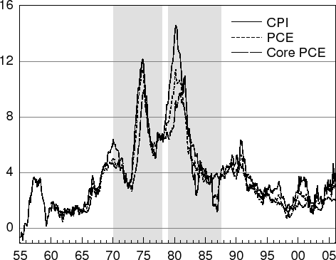 Note: Shaded areas correspond to the Burns and Volcker terms respectively. Source: CPI data from the Bureau of Labor Statistics, U.S. Department of Labor and PCE data from the Bureau of Economic Analysis, U.S. Department of Commerce. |
The approach taken here is an attractive alternative to the reaction-function estimations mentioned in the introduction, particularly in light of recent critique by Rudebusch (2002b) and Söderlind, Söderström, and Vredin (2005) that model mis-specification causes estimates of central-bank preferences based on these methods to be unreliable. The univariate framework proposed here has the advantage that the policy first-order condition is essentially the same regardless of which state variables are included in the model (Svensson, 1997), making the application more robust to a range of economic specifications.
3.1 Data
The model is estimated with U.S. inflation data, employing the monthly all goods Consumer Price Index (CPI) from 1955 to 2006 and the Personal Consumption Expenditure (PCE) deflator from the National Income and Product Accounts (NIPAs) from 1960 to 2006. The latter excludes interest sensitive components and is weighted together using chain-index methods. Core measures of inflation, particularly core PCE, have gained more attention from policy makers in recent years and we perform the analysis for core PCE. Figure 1 plots the data: twelve-month ended U.S. CPI, PCE and core PCE inflation.
3.2 CPI Estimation Results
The state-space model described by equations (9) and (10) is estimated with monthly observations of year-ended CPI inflation from January 1955 to January 2006. Table 1 reports the key coefficients, while the estimated series
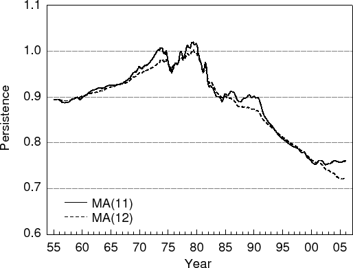
![]() is plotted as the solid line in Figure 2. Examining Figure 2, the pattern of time variation
in inflation persistence is largely consistent with a reading of Federal Reserve policy history, with inflation persistence high and more volatile during the 1970s than in surrounding years. The decline of inflation persistence immediately after Volcker became chairman in 1979 suggests that the
Federal Reserve became substantially more concerned with inflation stabilization. Persistence continued to decline toward the end of the sample, indicating strengthening focus on inflation stability during Greenspan's chairmanship. The estimate of the inflation target for the whole sample is 2.7
percent (reported in the first column of Table 1), reasonable for the most recent decade but lower than typically presumed for earlier years.7
is plotted as the solid line in Figure 2. Examining Figure 2, the pattern of time variation
in inflation persistence is largely consistent with a reading of Federal Reserve policy history, with inflation persistence high and more volatile during the 1970s than in surrounding years. The decline of inflation persistence immediately after Volcker became chairman in 1979 suggests that the
Federal Reserve became substantially more concerned with inflation stabilization. Persistence continued to decline toward the end of the sample, indicating strengthening focus on inflation stability during Greenspan's chairmanship. The estimate of the inflation target for the whole sample is 2.7
percent (reported in the first column of Table 1), reasonable for the most recent decade but lower than typically presumed for earlier years.7
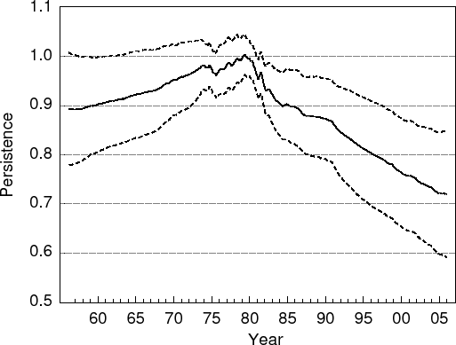 Notes: Estimates from an MA(12) error specification with twelve-month ended CPI data. The dashed lines are tex2html_wrap_inline$±$ two root mean square error bands. |
Judging from residual tests and information criteria, the MA(12) process for the errors is preferred over the MA(11) specification as well as over higher-order processes. The filtered series for the MA(12) process is shown as the dashed line in Figure 2. The profile of inflation persistence
closely resembles that of the MA(11) specification, but peaks and troughs are smoothed out and the number of occasions on which
![]() exceeds one is reduced substantially. The model is also preferred over the equivalent ARMA model with constant parameters, according to information criteria, indicating that
time variation in the persistence parameter is econometrically preferred over the static alternative. Figure 3 plots the MA(12) specification estimates along with two root mean-square error bands. From late 1981 and onwards, inflation persistence has been significantly less than one, judging by the
bands, and persistence today is significantly below that of the 1970s and early 1980s.
exceeds one is reduced substantially. The model is also preferred over the equivalent ARMA model with constant parameters, according to information criteria, indicating that
time variation in the persistence parameter is econometrically preferred over the static alternative. Figure 3 plots the MA(12) specification estimates along with two root mean-square error bands. From late 1981 and onwards, inflation persistence has been significantly less than one, judging by the
bands, and persistence today is significantly below that of the 1970s and early 1980s.
In the first quarter of 1979, the point estimate of persistence briefly exceeds one, the upper limit for a stabilizing central bank. The standard error bands are sufficiently wide for this not to be troubling, but it is worth considering some reasons that could generate such a result. First,
poorly anchored inflation expectations may have ratcheted up during inflationary episodes, as in the adaptive learning mechanism described in Orphanides and Williams (2003), thwarting attempts by the central bank to stabilize inflation and appearing temporarily as
explosive inflation persistence. Second, the Federal Reserve may have pursued different goals for the level of inflation at different times, distorting the estimation of the persistence parameter. Third, the Federal Reserve may have actively accommodated inflationary cost-push shocks, as suggested
by Kozicki and Tinsley (2005), raising the inflation target to alleviate the output trade-off. This may have been particularly true during oil-price shocks, as times when
![]() exceeds 1 coincide approximately with those episodes. We address
the latter two possibilities in Section 4.
exceeds 1 coincide approximately with those episodes. We address
the latter two possibilities in Section 4.
| CPI: MA(11) | CPI: MA(12) | PCE: MA(12) | Core PCE: MA(12) | |
|---|---|---|---|---|
|
|
2.721
|
2.826
|
2.430
|
1.791
|
|
|
(0.272) | (0.356) | (0.299) | (0.145) |
|
|
0.049 | 0.049 | 0.024 | 0.013 |
|
|
1.112x10 |
4.839x10 |
3.894x10 |
7.878x10 |
Notes: * (**) denotes significance at the 5 (1) percent level. Standard errors in parentheses.
3.3 PCE Deflator Estimation Results
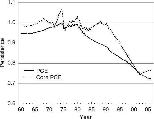 Notes: Estimates from an MA(12) error specification with twelve-month ended PCE data, January 1960 to January 2006. |
We estimate the MA(12) version of the state space model shown in equations (9) and (10) with year-ended changes in the PCE deflator and core PCE deflator (excluding food and energy) from the NIPAs.8 The third and fourth columns of Table 1 present results and Figure 4 plots the estimated paths of
![]() for both headline and core PCE inflation. The PCE data also prefer the MA(12) specification according to information criteria and tell a similar story to
the CPI data. The estimated inflation targets are 2.4 and 1.8 percent for headline
and core PCE inflation respectively, and the paths of persistence resemble closely those in Figure 2. Persistence trends down during Greenspan's term, reaching 0.765 (0.724) by the end of the sample for the headline (core) data - close to the end value estimated with CPI data (0.720). The series for core PCE evolves less smoothly, perhaps connected to its more recent availability. From late 1981, PCE persistence is also significantly less than one. Overall, these results provide further evidence of a pronounced
shift in the degree of inflation persistence in the United States.
for both headline and core PCE inflation. The PCE data also prefer the MA(12) specification according to information criteria and tell a similar story to
the CPI data. The estimated inflation targets are 2.4 and 1.8 percent for headline
and core PCE inflation respectively, and the paths of persistence resemble closely those in Figure 2. Persistence trends down during Greenspan's term, reaching 0.765 (0.724) by the end of the sample for the headline (core) data - close to the end value estimated with CPI data (0.720). The series for core PCE evolves less smoothly, perhaps connected to its more recent availability. From late 1981, PCE persistence is also significantly less than one. Overall, these results provide further evidence of a pronounced
shift in the degree of inflation persistence in the United States.
4 Extensions
In this section we consider shifts in the inflation target, a common means of modelling the big swings in inflation. Explanations that have been put forward for a time-varying inflation target include the different preferences of Federal Reserve Chairman (Clarida et al., 2000, Erceg and Levin, 2003), accommodation of supply shocks (Kozicki and Tinsley, 2005), opportunistic disinflation (Kuttner, 2004) or simply adaptation of the target to lagged inflation (Gürkaynak, Sack and Swanson, 2005). We investigate whether the evidence for time-varying inflation persistence remains when estimated in conjunction with a discretely shifting target. While it would be attractive to nest a gradually evolving target into our model of gradual persistence change, it introduces non-linearities into the model which make estimation infeasible with standard Kalman filter techniques. Thus in this paper, we specifically test for interactions of the target with the tenure of each chairman and the supply shocks that attract most attention, oil-price shocks.
| Chairman | Oil in target | |
|---|---|---|
|
|
2.890
|
2.848
|
|
|
(0.371) | (0.324) |
| -0.916 | - | |
| (0.610) | ||
| 4.242
|
- | |
| (1.289) | ||
| 5.659
|
- | |
| (1.343) | ||
| 0.149 | - | |
| (0.913) | ||
| - | 0.162 | |
| (1.656) | ||
| - | 4.149
|
|
| (1.494) | ||
| - | 1.951 | |
| (1.580) | ||
|
|
0.048 | 0.049 |
|
|
6.983x10 |
4.597x10 |
Notes: * (**) denotes significance at the 5 (1) percent level. Standard errors in parentheses.
4.1 Chairmen
Dummy variables for each Chairman's term capture discrete shifts in the target as follows:
 |
(11) |
This is preferred to splitting the data into sub-samples according to Chairman, as in Taylor (1999) and Clarida et al. (2000), which reduces sample length and decreases estimation precision. Results are reported in the first column of coefficients in Table 2. The reference estimate of the headline CPI inflation target is 2.9 percent during Greenspan's chairmanship. During Martin's chairmanship (January 1955 to January 1970), the target was slightly lower but not significantly different from that which prevailed under Greenspan. The estimated target rose substantially during the Burns and Miller periods (February 1970 to January 1978 and March 1978 to August 1979 respectively); under Burns, the target is estimated to have exceeded the Greenspan era by 4.2 percentage points and during Miller's short tenure, the inflation target moved higher. Volcker's tenure (August 1979 to August 1987) is marked by a substantial decrease in the target to a level statistically indistinguishable from that which prevailed under Greenspan.
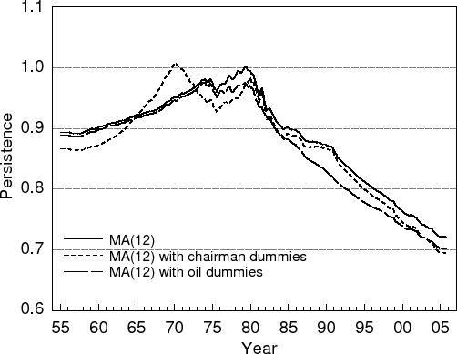 Notes: The solid line represents the MA(12) model presented in Figures 2 and 3 and the dotted lines shows persistence estimated as in equations (11) and (12). |
Overall, these results lend support to the idea that the Federal Reserve's inflation target may have changed over time, and the magnitude of the shifts in the target are consistent with the swings found by Ireland (2006) and Kozicki and Tinsley (2005). It is worth noting that despite permitting target shifts, clear evidence for the time-varying nature of inflation persistence remains (see Figure 5). Given this evidence for changing preferences regarding the level of inflation, it seems plausible that the preference for inflation stability has also evolved, and inflation persistence along with it. Information criteria slightly prefer the MA(12) specification with a constant target over the specification with dummy variables, but the two specifications are empirically almost indistinguishable.9
4.2 Oil Price Shocks
As discussed above, instances when the persistence parameter
![]() exceeds one are difficult to interpret in the context of the model. These episodes appear to coincide reasonably well with oil-price shocks centered around 1973, 1979 and 1990,
which may distort the estimates of inflation persistence either by introducing temporary changes in inflation dynamics or because the Federal Reserve accommodated the shocks in its target.
exceeds one are difficult to interpret in the context of the model. These episodes appear to coincide reasonably well with oil-price shocks centered around 1973, 1979 and 1990,
which may distort the estimates of inflation persistence either by introducing temporary changes in inflation dynamics or because the Federal Reserve accommodated the shocks in its target.
We create dummy variables for these episodes and use them to augment our previous MA(12) specification in Section 3. If the Federal Reserve has periodically ratcheted up the inflation target to accommodate inflationary oil-price shocks, we would expect to see significant interaction terms. The
dummy variables are as follows: ![]() from May 1973 to October 1974,
from May 1973 to October 1974, ![]() from
August 1978 to October 1981 and
from
August 1978 to October 1981 and ![]() from August 1990 to July 1991. Interacting the dummies with the inflation target, as in the following specification,
from August 1990 to July 1991. Interacting the dummies with the inflation target, as in the following specification,
yields a filtered series of
5 Implications for Policy-makers' Preferences
We motivated the empirical strategy of this paper by noting that in standard models of central-bank optimization, time variation in inflation persistence reflects the evolution of policy-makers' willingness to stabilize output. What do our estimates of inflation persistence imply then for
![]() ? In this section, we calibrate parameters of the model to imply an approximate range of values for
? In this section, we calibrate parameters of the model to imply an approximate range of values for ![]() consistent with estimated inflation persistence.
consistent with estimated inflation persistence.
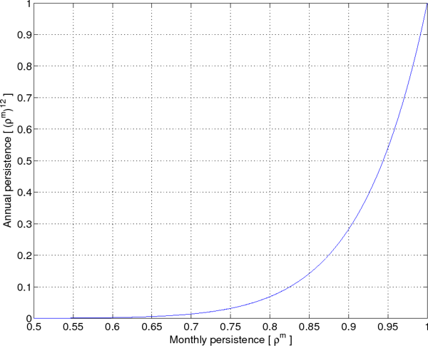
Through repeated substitution of the monthly persistence process in equation (7), annual persistence can be expressed as
![\displaystyle \pi _{t}-\pi ^{\ast }=\left[ \overset{11}{\underset{j=0}{\Pi }}\rho _{t-j}^{m}\right] \left( \pi _{t-12}-\pi ^{\ast }\right).](img86.gif) |
Persistence evolves slowly, so this calculation differs very little from simply computing
Because ![]() is a function of
is a function of ![]() ,
, ![]() ,
, ![]() ,
, ![]() and
and ![]() , assumptions about the first four parameters are needed in order to map
, assumptions about the first four parameters are needed in order to map ![]() to
to ![]() . We employ the standard assumption that the central bank discounts very little and thus choose
. We employ the standard assumption that the central bank discounts very little and thus choose
![]() . Following Clarida et al. (1999), we also set
. Following Clarida et al. (1999), we also set ![]() equal to this value. With respect to the output elasticity in the Phillips curve,
equal to this value. With respect to the output elasticity in the Phillips curve, ![]() , estimates in the literature range from 0.3 (Rudebusch, 2002) to 0.15 (Dennis, 2006) to 0.05 (Galí, Gertler and Lopez-Salido, 2001). In line with these findings, we infer values for
, estimates in the literature range from 0.3 (Rudebusch, 2002) to 0.15 (Dennis, 2006) to 0.05 (Galí, Gertler and Lopez-Salido, 2001). In line with these findings, we infer values for ![]() conditional on two values of
conditional on two values of ![]() ,
,
![]() .
.
The model presented here is sufficiently general to encompass a wide range of views about the degree of forward and backward lookingness in the Phillips curve, regulated by ![]() . Estimated
hybrid models tend to find most weight attached to lagged variables in the New-Keynesian Phillips Curve, such as Rudebusch and Svensson (1999) and Rudebusch (2002a), but the issue remains disputed (see Henry and Pagan (2004), Gali et al (2001), and Rudd and Whelan (2005) for recent, and diverse, opinions on this topic). To accommodate these viewpoints, we map inflation persistence to
. Estimated
hybrid models tend to find most weight attached to lagged variables in the New-Keynesian Phillips Curve, such as Rudebusch and Svensson (1999) and Rudebusch (2002a), but the issue remains disputed (see Henry and Pagan (2004), Gali et al (2001), and Rudd and Whelan (2005) for recent, and diverse, opinions on this topic). To accommodate these viewpoints, we map inflation persistence to ![]() for four different values of
for four different values of ![]() ranging from strongly forward looking to completely
backward looking,
ranging from strongly forward looking to completely
backward looking,
![]() .
.
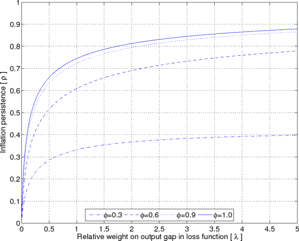
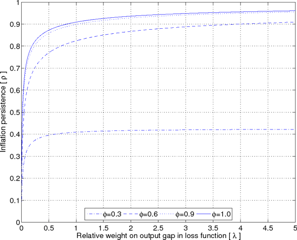
Given our parameter assumptions, Figures 7 and 8 map inflation persistence into values for ![]() . Each line represents a
different value of
. Each line represents a
different value of ![]() and confirms the intuition that inflation persistence is higher for more backward-looking parameterizations. For each line, inflation persistence is a monotonically
increasing function of the relative preference for output stability.
and confirms the intuition that inflation persistence is higher for more backward-looking parameterizations. For each line, inflation persistence is a monotonically
increasing function of the relative preference for output stability.
The MA(12) specification yielded average annual inflation persistence over the Volcker-Greenspan era of 0.12/0.14/0.29 for CPI/PCE/core PCE respectively. These imply unambiguously low values of the preference for output stability. For most parameter combinations, the values of ![]() corresponding to these levels of persistence are clustered between zero and 0.1. Only
with a substantial degree of forward lookingness (
corresponding to these levels of persistence are clustered between zero and 0.1. Only
with a substantial degree of forward lookingness (![]() ), could
), could ![]() be as
high as 0.6. Persistence at the end of Greenspan's tenure implies even lower values for the preference for output stability:
be as
high as 0.6. Persistence at the end of Greenspan's tenure implies even lower values for the preference for output stability: ![]() is judged to be less than 0.02 for all parameterizations.
This is in line with the findings of other researchers - including Favero and Rovelli (2003) and Söderlind et al. (2005) - that in recent samples,
is judged to be less than 0.02 for all parameterizations.
This is in line with the findings of other researchers - including Favero and Rovelli (2003) and Söderlind et al. (2005) - that in recent samples, ![]() is
not significantly different from zero and must be very small in calibrations to match U.S. inflation data.
is
not significantly different from zero and must be very small in calibrations to match U.S. inflation data.
During the 1970s, there was more dispersion in estimated inflation persistence across the three measures of inflation; 0.74/0.83/1.07 for CPI/PCE/core PCE respectively. To facilitate comparison, consider the central estimate, ![]() equal to 0.83. From Figure 8,
equal to 0.83. From Figure 8, ![]() must be 0.3 or greater to generate such persistence. With a higher elasticity of inflation with respect to
the output gap (Figure 7), correspondingly higher values of
must be 0.3 or greater to generate such persistence. With a higher elasticity of inflation with respect to
the output gap (Figure 7), correspondingly higher values of ![]() generate the same inflation persistence; the purely backward-looking case provides a lower bound of 2.5, with much larger
values for more forward-looking Phillips curves. Greater dispersion and higher inflation persistence are consistent with a wider range of
generate the same inflation persistence; the purely backward-looking case provides a lower bound of 2.5, with much larger
values for more forward-looking Phillips curves. Greater dispersion and higher inflation persistence are consistent with a wider range of ![]() but these values nonetheless map to higher
values of
but these values nonetheless map to higher
values of ![]() . According to the model we began with in Section 2, this implies that the preference for inflation stability was weaker during this period than in surrounding years.
. According to the model we began with in Section 2, this implies that the preference for inflation stability was weaker during this period than in surrounding years.
Summing up, implied values of ![]() span a broad range for the 1970s and a narrower, lower range for the Volcker-Greenspan period. For each measure of price inflation, the decline in
average persistence implies substantially stronger preferences for inflation stability and by the end of the sample, the inferred value of
span a broad range for the 1970s and a narrower, lower range for the Volcker-Greenspan period. For each measure of price inflation, the decline in
average persistence implies substantially stronger preferences for inflation stability and by the end of the sample, the inferred value of ![]() is clearly outside the range during the
1970s.10
is clearly outside the range during the
1970s.10
There are several important caveats to this exercise. First, uncertainty around the point estimates and the choice of calibration values makes an exact range for ![]() difficult to pin
down. The inferences should be treated as indicative only. Second, time variation in other parameters - namely
difficult to pin
down. The inferences should be treated as indicative only. Second, time variation in other parameters - namely ![]() ,
, ![]() ,
, ![]() and
and ![]() - would be mistakenly
attributed by our identification to the preference for output stability. For example, an increase in the elasticity of inflation with respect to the output gap (higher
- would be mistakenly
attributed by our identification to the preference for output stability. For example, an increase in the elasticity of inflation with respect to the output gap (higher ![]() ) or increasingly
forward-looking behavior in the Phillips curve (lower
) or increasingly
forward-looking behavior in the Phillips curve (lower ![]() ) would, all else constant, reduce inflation persistence in the economy. Concerning
) would, all else constant, reduce inflation persistence in the economy. Concerning ![]() and
and ![]() , we have little reason to believe that these parameters have changed substantially. In addition, evidence that
the Phillips curve appears to have been stable over time (Dupuis, 2004 and Lindé, 2005) lessens our concern about time variation in
, we have little reason to believe that these parameters have changed substantially. In addition, evidence that
the Phillips curve appears to have been stable over time (Dupuis, 2004 and Lindé, 2005) lessens our concern about time variation in ![]() and/or
and/or ![]() .
.
There are other factors outside the scope of the model that could also generate changes in inflation persistence without reflecting changes in policy preferences. As pointed out by Svensson (1999), model uncertainty - in particular, uncertainty about the natural rate - and interest-rate smoothing could both give rise to more gradual adjustment of conditional inflation forecasts back to the target. It is difficult to assess how the degree of model uncertainty has changed over the course of our sample; if the degree of uncertainty about the natural rate has remained roughly constant, then inference about the direction of change in Federal Reserve's preferences is unaffected. If model uncertainty has in fact declined, this may account for some of the decline in inflation persistence.
Regarding interest rate smoothing, we observe less inflation persistence during the last 15 years of the sample, but many economists believe these years were a time when greater emphasis was placed on the smooth adjustment of interest rates. The observed decline in inflation persistence could
either imply that ![]() there has been minimal movement toward interest-rate smoothing, or that
there has been minimal movement toward interest-rate smoothing, or that ![]() the decline in the relative preference for output stability has been even more pronounced, offsetting the effect of a shift toward interest-rate smoothing on inflation persistence. Lastly, growing credibility of the central bank's nominal anchor may have facilitated faster mean
reversion of the public's inflation expectations following shocks and contributed to the estimated decline in persistence.
the decline in the relative preference for output stability has been even more pronounced, offsetting the effect of a shift toward interest-rate smoothing on inflation persistence. Lastly, growing credibility of the central bank's nominal anchor may have facilitated faster mean
reversion of the public's inflation expectations following shocks and contributed to the estimated decline in persistence.
6 Conclusions
Starting with a standard model of the macroeconomy, we have argued that if the Federal Reserve's preference for output stability has varied over time, this should be observable in inflation persistence. By estimating an ARMA(1,q) model with time-varying persistence parameter, we find that
inflation persistence has indeed exhibited significant swings. Moreover, the estimation results are plausible. Consistent with the general opinion that inflation stability was given more focus during Volcker's chairmanship, inflation persistence fell during the 1980s and continued to do so during
Greenspan's term. Inflation persistence today is both significantly less than one and significantly different from that which prevailed in the 1970s and early 1980s. With attention paid to moving-average disturbances and oil price shocks, estimates also stay within the
![]() range considered plausible in the model.
range considered plausible in the model.
In our baseline specification, the headline CPI inflation target is estimated to have been approximately 2.8 percent since the mid-1950s and slightly lower for PCE and core PCE inflation, 2.4 and 1.8 percent respectively. The combination of a stable inflation target and time-varying inflation persistence suggests that high inflation of the past was due to the unwillingness to stabilize inflation rather than substantially higher inflation goals. By the same logic, inflation goals were reached during the 1990s because of a greater willingness to stabilize inflation at the cost of output stability. Augmenting the model with chairman-specific inflation targets indicates that the inflation target was likely higher during Burns' and Miller's tenures. Regardless of specification, inflation persistence is clearly observed to have risen and fallen.11
A low inflation target paired with time-varying inflation persistence is also consistent with the stylized facts of the falling level and volatility of inflation during the last two decades. Modelling the inflation process with shifts in its target or intercept, as in Kozicki and Tinsley (2005) and Levin and Piger (2002), can explain changes in the level of inflation but not its variance. In contrast, declining inflation persistence in conjunction with a stable target coincides with the lower level and volatility of inflation toward the end of our sample.
Our findings are consistent with the interpretation of Clarida et al. (2000), among others, who argue that larger estimated coefficients on inflation in reaction functions for later samples indicate a greater willingness to stabilize inflation at the cost of output. Our results also echo the findings of Primiceri (2005), that steady state inflation rates and the target have been low and stable since the 1960s. We differ from Primiceri's interpretation, however, that prolonged periods of high inflation were due to central-bank misunderstandings about the natural rate and parameters of the Phillips curve; in our model, prolonged inflation results from a high preference for output stability. Reconciling these two interpretations is an interesting topic for future research and could take the form of modelling the interaction between central-bank preferences and learning about macroeconomic parameters.
From a broader perspective, our results are also relevant to the literature on the empirical time-series properties of inflation. Our findings contrast with the viewpoint that inflation has a unit root, as argued by Mishkin (1992) and Crowder and Hoffman (1996), and with findings that inflation persistence has been stable (see Levin and Piger (2002) employing an AR model with intercept shifts and Pivetta and Reis (2006) using rolling regressions). With few exceptions, our point estimates of the persistence parameter are less than one, implying that inflation is mean reverting (but not covariance-stationary, as the speed of mean reversion changes over time). The approach we employ is sufficiently flexible to permit the properties of inflation to change between integrated and mean-reverting over the sample, unlike the traditional dichotomy in the unit-root literature of classifying inflation as I(0) or I(1), and better able to detect small and gradual changes in inflation persistence than rolling regressions.


![k(\lambda )=\frac{1}{2}\left[ 1-\frac{% \lambda (1-\delta )}{\delta \alpha _{y}^{2}}+\sqrt{\left( 1+\frac{\lambda (1-\delta )}{\delta \alpha _{y}^{2}}\right) ^{2}+\frac{4\lambda }{\alpha _{y}^{2}}}\right] \geq 1](img33.gif)