Skip to: [Printable Version (PDF)] [Bibliography] [Footnotes]

Finance and Economics Discussion Series: 2007-34 Screen Reader version ^♣

News, Noise, and Estimates of the "True" Unobserved State of the Economy

Dennis J. Fixler and Jeremy J. Nalewaik*

Revised September 18, 2007

Keywords: GDP, statistical discrepancy, news and noise, signal-to-noise ratios, optimal combination of estimates, business cycles

Abstract:

Which provides a better estimate of the "true" state of the U.S. economy, gross domestic product (GDP) or gross domestic income (GDI)? Past work has assumed the idiosyncratic variation in each estimate is pure noise, taking greater variability to imply lower reliability. We develop models that relax this assumption, allowing the idiosyncratic variation in the estimates to be partly or pure news; then greater variability may imply higher information content and greater reliability. Based on evidence from revisions, we reject the pure noise assumption for GDI growth, and our results favor placing a higher weight on GDI due to its relatively large idiosyncratic variability. This calls into question the suitability of the pure noise assumption in other contexts, including dynamic factor models.

JEL classification: C1, C82.

1 Introduction

For analysts of economic fluctuations, estimating the true state of the economy from imperfectly measured official statistics is an ever-present problem. As most economists agree that no one statistic is a perfect gauge of the state of the economy, many have proposed using some type of weighted average of multiple imperfectly measured statistics instead. Examples include the composite index of coincident indicators,¹ and averages of different measures of aggregate economic activity such as gross domestic product (GDP) and its income-side counterpart GDI. While the precise meaning of the state of the economy can vary from case to case, in this paper we take it to mean the growth rate of the size of the economy as traditionally defined in the U.S. National Income and Product Accounts (NIPAs).² $^{,}$ ³

The main point of our paper is as follows. To our knowledge, all prior attempts to produce such a weighted average of imperfectly measured statistics have made a strong implicit assumption that drives their weighting: that the idiosyncratic variation in each measured statistic is pure noise, or completely uncorrelated with information about the true state of the economy.⁴ Under this assumption, a statistic with greater idiosyncratic variance is given a smaller weight because it is assumed to contain more noise. We consider the implications of relaxing this assumption, allowing the idiosyncratic variation in each measured statistic to contain news, or information about the true state of the economy. If the idiosyncratic variation is mostly news, the implied weighting is diametrically opposite that of the noise assumption: a statistic with greater idiosyncratic variance should be given a larger weight because it contains more information about the true state of the economy. The implicit noise assumption relied upon in numerous prior papers is arbitrary, and more information must be brought to bear on this issue.

Focusing on GDP and GDI allows us to make this basic point in a simple bivariate context. These two measures of the size of the U.S. economy would equal one another if all the transactions in the economy were observed, but measurement difficulties lead to the statistical discrepancy between the two; their quarterly growth rates often diverge significantly. Weale (1992) and others⁵ have estimated the growth rate of "true" unobserved GDP as a combination of measured GDP growth and GDI growth, generally concluding that GDI growth should be given more weight than measured GDP growth. Is GDI really the more accurate measure? We argue for caution, as the results are driven entirely by the noise assumption: the models implicitly assume that since GDP growth has higher variance than GDI growth over their sample period, it must be noisier, and so should receive a smaller weight. However GDP may have higher variance because it contains more information about "true" unobserved GDP (this is the essence of the news assumption); then measured GDP should receive the higher weight.

In the general version of our model that allows the idiosyncratic component of each measured statistic to be a mixture of news and noise, virtually any set of weights can be rationalized by making untestable assumptions about the mixtures. More information must be brought to bear on the problem; otherwise the choice of weights will be arbitrary. This point is broadly applicable, extending well beyond the simple bivariate case of GDP and GDI. For example, a large and growing literature on dynamic factor models uses principal components or other methods to extract common factors out of large data sets; see Stock and Watson (2002), Forni, Hallin, Lippi, and Reichlin (2000), Bernanke and Boivin (2003), Giannone, Reichlin, and Small (2005), Bernanke, Boivin, and Eliasz (2005), and Boivin and Ng (2006).⁶ While often these common factors are used for pure forecasting, sometimes they are equated with unobserveables of interest, assuming the idiosyncratic components of the variables in the dataset are uninteresting noise. However if these idiosyncratic components do contain useful information about the unobserveables of interest, estimating the unobserveables optimally may require taking weighted averages of the variables in the dataset very different from those implied by the factor models.

While this fundamental indeterminancy - the arbitrary nature of most weighting schemes - is somewhat disturbing, in the case of combining GDP and GDI we bring more information to bear on the problem to help pin down the weights. GDI growth has more idiosyncratic variation than GDP growth in the sample we employ, which starts in the mid 1980s after the marked reduction in the variance of the measured estimates - see McConnell and Perez-Quiros (2000). However the initial GDI growth estimates have negligible idiosyncratic variance; it is only through revisions that the idiosyncratic variance of GDI growth becomes relatively large. If the revisions add news, and not noise - an assumption that is consistent with our knowledge of the revisions process and that follows previous research such as Mankiw, Runkle and Shapiro (1984) and Mankiw and Shapiro (1986) - then there must be a strong presumption that the idiosyncratic variation in GDI growth is largely news, news derived from the revisions.

We decompose the revisions to GDP and GDI growth into news and noise, show how to place bounds on the shares of their idiosyncratic variances that are news, and based on these bounds we test the assumptions of the pure noise model, rejecting them at conventional significance levels. Based on its relatively large idiosyncratic variation, GDI growth should be weighted more heavily, not less, in estimating "true" unobserved GDP growth. This leads to some interesting modifications of economic history: for example both before and after the 1990-1991 recession, economic growth is weaker than indicated by measured GDP growth. Furthermore, our results indicate that measured GDP growth understates the true variability of the economy's growth rate, a fact with clear implications for real business cycle, asset pricing, and other models.

2 Theory: The Competing News and Noise Models

2.1 Review of News and Noise

Let $\Delta y_{t}^{\star}$ be the true growth rate of the economy, let $\Delta y_{t}^{i}$ be one of its measured estimates, and let $\varepsilon_{t}^{i}$ be the difference between the two, so:

$\displaystyle \Delta y_{t}^{i} = \Delta y_{t}^{\star}+ \varepsilon_{t}^{i}.$

The noise model makes the classical measurement error assumption that $\operatorname{cov}\left( \Delta y_{t}^{\star},\varepsilon_{t}^{i}\right) = 0$ ; this is the precise meaning of the statement that $\varepsilon_{t}^{i}$ is noise. One implication of a noisy estimate $\Delta y_{t}^{i}$ is that it's variance is greater than the variance of the true growth rate of the economy, or $\operatorname{var}\left( \Delta y_{t}^{i}\right) > \operatorname{var}\left( \Delta y_{t}^{\star}\right)$ .

In contrast, if an estimate $\Delta y_{t}^{i}$ were constructed efficiently with respect to a set of information about $\Delta y_{t}^{\star}$ (call it $\mathcal{F}_{t}^{i}$ ), then $\Delta y_{t}^{i}$ would be the conditional expectation of $\Delta y_{t}^{\star}$ given that information set:

$\displaystyle \Delta y_{t}^{i}$

$\displaystyle = E\left( \Delta y_{t}^{\star}\vert \mathcal{F}_{t}^{i} \right) .$

Writing:

$\displaystyle \Delta y_{t}^{\star}$

$\displaystyle = \Delta y_{t}^{i} + \zeta_{t}^{i},$

the term $\zeta_{t}^{i}$ represents the information about $\Delta y_{t}% ^{\star}$ that is unavailable in the construction of $\Delta y_{t}^{i}$ . Then $\Delta y_{t}^{i}$ and $\zeta_{t}^{i}$ represent mutually orthogonal pieces of news about $\Delta y_{t}^{\star}$ , employing the terminology in Mankiw and Shapiro (1986), and $\operatorname{cov}\left( \Delta y_{t}% ^{i},\zeta_{t}^{i}\right) = 0$ . This leads us to an implication of the news model that we employ later, namely that $\operatorname{cov}\left( \Delta y_{t}^{i},\Delta y_{t}^{\star}\right) =\operatorname{var}\left( \Delta y_{t}^{i}\right)$ . We also have $\operatorname{var}\left( \Delta y_{t}% ^{\star}\right) > \operatorname{var}\left( \Delta y_{t}^{i}\right)$ , an implication opposite to that of the noise model.

These two models are clearly extremes; the next section considers a general model that allows differing degrees of news and noise in the estimates.

2.2 The Mixed News and Noise Model

We consider a model with two estimates of true unobserved GDP growth, each an efficient estimate plus noise:

	$\displaystyle \Delta y_{t}^{1}$	$\displaystyle = E\left( \Delta y_{t}^{\star}\vert \mathcal{F}_{t}^{1} \right) + \varepsilon_{t}^{1},$ and
	$\displaystyle \Delta y_{t}^{2}$	$\displaystyle = E\left( \Delta y_{t}^{\star}\vert \mathcal{F}_{t}^{2} \right) + \varepsilon_{t}^{2}.$

The noise components $\varepsilon_{t}^{1}$ and $\varepsilon_{t}^{2}$ are mutually uncorrelated and, naturally, uncorrelated with true unobserved GDP. Taking $\Delta y_{t}^{1}$ to be GDP and $\Delta y_{t}^{2}$ to be GDI, the information in $\mathcal{F}_{t}^{1}$ likely would consist of personal consumption expenditures, investment, net exports, and the other components that sum to GDP, while the information in $\mathcal{F}_{t}^{2}$ likely would consist of wage and salary income, corporate profits, proprietors' income, and the other components that sum to GDI.⁷ We assume each information set includes a constant, so both $\Delta y_{t}^{1}$ and $\Delta y_{t}^{2}$ consistently estimate the mean $\mu$ of $\Delta y_{t}^{\star}$ , and there may be a substantial amount of additional overlap between the two information sets. Consumption growth may be highly correlated with the growth rate of wages and salaries, for example. However a key feature of our model is that it recognizes that the two information sets are not necessarily identical.⁸

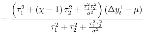
To clearly illustrate the main points of the paper, we focus on the simple case where all variables are jointly normally distributed, and where measured GDP and GDI are serially uncorrelated.⁹ With normality, the conditional expectation of the true growth rate of the economy is a weighted average of GDP and GDI; netting out means yields:

	$\displaystyle E\left( \Delta y_{t}^{\star}- \mu\vert \Delta y_{t}^{1}, \Delta y_{t}^{2}, \mu\right)$	$\displaystyle =$
(1')	$\displaystyle \widehat{\Delta y_{t}^{\star}} - \mu$	$\displaystyle = \omega_{1} \left( \Delta y_{t}^{1} - \mu\right) + \omega_{2} \left( \Delta y_{t}^{2} - \mu\right) ,$

calling the conditional expectation $\widehat{\Delta y_{t}^{\star}}$ . The weights $\omega_{i}$ can be derived using standard formulas for the population version of ordinary least squares:

(2')	$\displaystyle \left( \begin{array}[c]{c}% \omega_{1}\ \omega_{2}% \end{array} \right)$	$\displaystyle = \left( \begin{array}[c]{cc}% \operatorname{var}\left( \Delta y_{t}^{1}\right) & \operatorname{cov}\left( \Delta y_{t}^{1},\Delta y_{t}^{2}\right) \ \operatorname{cov}\left( \Delta y_{t}^{1},\Delta y_{t}^{2}\right) & \operatorname{var}\left( \Delta y_{t}^{2}\right) \end{array} \right) ^{-1} \left( \begin{array}[c]{c}% \operatorname{cov}\left( \Delta y_{t}^{1},\Delta y_{t}^{\star}\right) \ \operatorname{cov}\left( \Delta y_{t}^{2},\Delta y_{t}^{\star}\right) \end{array} \right)$
		$\displaystyle = \left( \begin{array}[c]{cc}% \operatorname{var}\left( \Delta y_{t}^{1}\right) & \operatorname{cov}\left( \Delta y_{t}^{1},\Delta y_{t}^{2}\right) \ \operatorname{cov}\left( \Delta y_{t}^{1},\Delta y_{t}^{2}\right) & \operatorname{var}\left( \Delta y_{t}^{2}\right) \end{array} \right) ^{-1} \left( \begin{array}[c]{c}% \operatorname{var}\left( E\left( \Delta y_{t}^{\star}\vert \mathcal{F}_{t}^{1} \right) \right) \ \operatorname{var}\left( E\left( \Delta y_{t}^{\star}\vert \mathcal{F}_{t}^{2} \right) \right) \end{array} \right) ,$

using $\operatorname{cov}\left( \Delta y_{t}^{\star},\varepsilon_{t}% ^{i}\right) = 0$ and the property of efficient estimates that their covariance with the variable they estimate is simply their variance.

It is useful to introduce some additional notation. Call the covariance between the two estimates $\sigma^{2}$ ; this arises from the overlap between the information sets used to compute the efficient estimates, and correlation between the measurement errors $\varepsilon_{t}^{1}$ and $\varepsilon_{t}^{2}%$ . The model imposes the condition that the variance of each estimate is at least as large as their covariance; let $\sigma^{2} + \tau^{2}_{1}$ and $\sigma^{2} + \tau^{2}_{2}$ be the variances of the $\Delta y_{t}^{1}$ and $\Delta y_{t}^{2}$ , respectively. The idiosyncratic variance in each estimate, the $\tau^{2}_{i}$ for , arises from two potential sources. The first source is the idiosyncratic news in each estimate - the information in each efficient estimate missing from the other, and the second source is noise.

Let the share of the covariance between the two estimates that is news, or common information, be $\chi$ . Similarly, let the news share of the idiosyncratic variance in the th estimate be $\chi_{i}$ , so $\left( 1-\chi_{i}\right)$ is the fraction of the idiosyncratic variance that is noise. Then equation (2) becomes:

$\displaystyle \left( \begin{array}[c]{c}% \omega_{1}\ \omega_{2}% \end{array} \right)$

$\displaystyle = \left( \begin{array}[c]{cc}% \sigma^{2} + \tau^{2}_{1} & \sigma^{2}\ \sigma^{2} & \sigma^{2} + \tau^{2}_{2}% \end{array} \right) ^{-1} \left( \begin{array}[c]{c}% \chi\sigma^{2} + \chi_{1} \tau^{2}_{1}\ \chi\sigma^{2} + \chi_{2} \tau^{2}_{2}% \end{array} \right) .$

Solving and substituting into (2) gives:

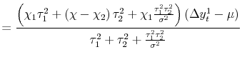	$\displaystyle \widehat{\Delta y_{t}^{\star}} - \mu$	$\displaystyle = \frac{\left( \chi_{1}\tau_{1}^{2} + \left( \chi-\chi_{2}\right) \tau_{2}^{2} + \chi_{1}\frac{\tau_{1}^{2}\tau _{2}^{2}}{\sigma^{2}}\right) \left( \Delta y_{t}^{1} - \mu\right) }{\tau _{1}^{2} + \tau_{2}^{2} + \frac{\tau_{1}^{2}\tau_{2}^{2}}{\sigma^{2}}% }$
(3')		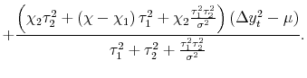$\displaystyle + \frac{\left( \chi_{2}\tau_{2}^{2} + \left( \chi-\chi_{1}\right) \tau _{1}^{2} + \chi_{2}\frac{\tau_{1}^{2}\tau_{2}^{2}}{\sigma^{2}}\right) \left( \Delta y_{t}^{2} - \mu\right) }{\tau_{1}^{2} + \tau_{2}^{2} + \frac{\tau _{1}^{2}\tau_{2}^{2}}{\sigma^{2}}}.$

Before examing (3) in greater depth, note that the weights on the two component variables here do not necessarily sum to one; the weights on the two components variables and mean $\mu$ sum to one. But in some situations the econometrician may have little confidence in the estimated mean $\mu$ , so it may be inadvisable to use it as the third component in the weighted average. One way around this problem is to force the weights on $\Delta y_{t}^{1}$ and $\Delta y_{t}^{2}$ to sum to one, with $\omega_{2} = 1 - \omega_{1}$ ; substituting into (1) and rearranging yields:

(1')

$\displaystyle E\left( \Delta y_{t}^{\star}- \Delta y_{t}^{2} \vert \Delta y_{t}^{1}, \Delta y_{t}^{2} \right)$

$\displaystyle = \omega_{1} \left( \Delta y_{t}^{1} - \Delta y_{t}^{2} \right) .$

Adding back in $\Delta y_{t}^{2}$ to equation (1') yields $\widehat{\Delta y_{t}^{\star}}$ . The solution to the general model then becomes:

(3')

$\displaystyle \widehat{\Delta y_{t}^{\star}}$

$\displaystyle = \frac{\left( \chi_{1}\tau_{1}^{2} + \left( 1-\chi_{2}\right) \tau_{2}^{2}\right) \Delta y_{t}^{1} + \left( \chi_{2}\tau_{2}^{2} + \left( 1-\chi_{1}\right) \tau_{1}^{2} \right) \Delta y_{t}^{2}}{\tau_{1}^{2} + \tau_{2}^{2}}.$

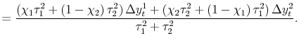With the assumptions of the pure noise model discussed below, this particular estimator is equivalent to the estimator proposed by Weale (1992) and Stone et al (1942). Appendix A clarifies the relation between these earlier estimators and those derived here.

It is clear that not all of the parameters of the unconstrained model are identified: we observe three moments from the variance-covariance matrix of $\left[ \Delta y_{t}^{1} \quad\Delta y_{t}^{2} \right]$ , which is not enough to pin down the six parameters $\sigma^{2}$ , $\tau_{1}^{2}$ , $\tau_{2}^{2}$ , $\chi$ , $\chi_{1}$ , and $\chi_{2}$ . Imposing values for $\chi$ , $\chi_{1}$ , and $\chi_{2}$ allows identification of the remaining parameters. Some illuminating special cases are examined next, which show how assumptions about the idiosyncratic news shares $\chi_{1}$ and $\chi_{2}$ are critical for determining the relative weights on the two component variables.

2.2.1 The Pure Noise Model

Previous attempts to estimate models of this kind have focused on one particular assumption for the idiosyncratic news shares: $\chi_{1} = \chi_{2} = 0$ . The implication is that the two information sets must coincide, at least in the universe of information that is relevant for predicting $\Delta y_{t}^{\star}$ , so $E\left( \Delta y_{t}^{\star}\vert \mathcal{F}_{t}^{1} \right) = E\left( \Delta y_{t}^{\star}\vert \mathcal{F}_{t}^{2} \right)$ . We call this the pure noise model; equation (3) is then:¹⁰

(4)	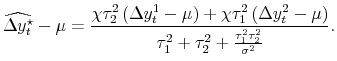$\displaystyle \widehat{\Delta y_{t}^{\star}} - \mu= \frac{\chi\tau_{2}^{2}\left( \Delta y_{t}^{1} - \mu\right) + \chi\tau_{1}^{2}\left( \Delta y_{t}^{2} - \mu\right) }{\tau_{1}^{2} + \tau_{2}^{2} + \frac{\tau_{1}^{2}\tau_{2}^{2}}{\sigma^{2}}}.$

In the pure noise model, the weight for one measure is proportional to the idiosyncratic variance of the other measure - since the idiosyncratic variance in each estimate is assumed to be noise, the "noisier" measure is downweighted. The weights on the (net of mean) estimates sum to less than one; as is typical in the classical measurement error model, coefficients on noisy explanatory variables are downweighted. In fact, as the common variance $\sigma^{2}$ approaches zero, the signal-to-noise ratio in the model approaches zero as well, and the formula instructs us to give up on the estimates of GDP and GDI for any given time period, using the overall sample mean as the best estimate for each and every period.

2.2.2 The Pure News Model

The opposite case is what we call the pure news model, where $\chi_{1} = \chi_{2} = 1$ . Equation (3) then becomes:

	$\displaystyle \widehat{\Delta y_{t}^{\star}} - \mu$	$\displaystyle = \frac{\left( \tau_{1}^{2} + \left( \chi-1\right) \tau_{2}^{2} + \frac{\tau_{1}^{2}\tau_{2}^{2}}{\sigma^{2}% }\right) \left( \Delta y_{t}^{1} - \mu\right) }{\tau_{1}^{2} + \tau_{2}^{2} + \frac{\tau_{1}^{2}\tau_{2}^{2}}{\sigma^{2}}}$
(5)		$\displaystyle + \frac{\left( \tau_{2}^{2} + \left( \chi-1\right) \tau_{1}^{2} + \frac{\tau_{1}^{2}\tau_{2}^{2}}{\sigma^{2}}\right) \left( \Delta y_{t}^{2} - \mu\right) }{\tau_{1}^{2} + \tau_{2}^{2} + \frac{\tau_{1}^{2}\tau_{2}^{2}% }{\sigma^{2}}}.$

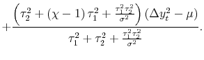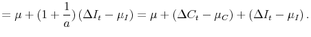
The weight for each measure is now proportional to its own idiosyncratic variance - the estimate with greater variance contains more news and hence receives a larger weight. This result is diametrically opposed to that of the noise model.

Under some circumstances it may be reasonable to assume that the covariance between the estimates is pure news, in which case the $\left( \chi-1\right)$ terms vanish; then the weights (on the net of mean estimates) sum to a number greater than unity, again opposite the pure noise model. As $\sigma^{2} \rightarrow0$ (i.e. as the variance common to the two estimates approaches zero), the weight for each estimate approaches unity. In this case, we are essentially adding together two independent pieces of information about GDP growth. To illustrate, suppose we receive news of a shock that moves $\Delta y_{t}^{\star}$ two percent above its mean, and then receive news of another, independent shock that moves $\Delta y_{t}^{\star}$ one percent below its mean. The logical estimate of $\Delta y_{t}^{\star}$ is then the mean plus one percent - i.e. the sum of the two shocks. In Appendix B we work through another example, of two estimates of GDP growth, each based on the growth rate of a different sector of the economy; if the growth rates of the sectors are uncorrelated, we simply add up the net-of-mean contributions to GDP growth of the two sectors, and then add back in the mean.

2.2.3 Arbitrary Weights

Finally, consider another case of interest: if $\chi_{i} = \chi$ and $\chi_{j} = 0$ , then $\omega_{i} = \chi$ and $\omega_{j} = 0$ , placing all the weight on variable . If placing all the weight on either variable can be justified with such assumptions about the idiosyncratic news shares, perhaps any set of weights is possible. This turns out to be the case. Let the ratio of the weights $\frac{\omega_{1}}{\omega_{2}} = r$ , so:

(6)

$\displaystyle r\left( \chi,\chi_{1},\chi_{2}\right) = \frac{\chi_{1}\tau_{1}^{2} + \left( \chi-\chi_{2}\right) \tau_{2}^{2} + \chi_{1}\frac{\tau_{1}^{2}\tau_{2}^{2}% }{\sigma^{2}}}{\chi_{2}\tau_{2}^{2} + \left( \chi-\chi_{1}\right) \tau_{1}^{2} + \chi_{2}\frac{\tau_{1}^{2}\tau_{2}^{2}}{\sigma^{2}}},$

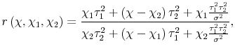
where we've expressed

as a function of $\chi$ , $\chi_{1}$ and $\chi_{2}$ . The following proposition shows that, for any $0 < \chi\le1$ , any set of weights can be rationalized by making untestable assumptions about the degree of news and noise in the idiosyncratic components of the two variables:

Proposition 1 Let be any non-negative real number, and let $r\left( \chi,\chi_{1}% ,\chi_{2} \right)$ be given by (6), where $\tau_{1}^{2}$ , $\tau_{2}^{2}$ , and $\sigma^{2}$ are each constant, positive real numbers, and $0 < \chi\le1$ . Then there exists a pair $\left( \chi_{1}^{\star},\chi_{2}^{\star }\right)$ , with $\chi_{1}^{\star} \in\left[ 0,\quad1\right)$ and $\chi _{2}^{\star} \in\left( 0,\quad1\right]$ , such that $r\left( \chi_{1}^{\star },\chi_{2}^{\star}\right) = r$ .

Proof: Consider an example that meets the conditions of the proposition, where $\chi_{2} = \chi- \chi_{1}$ . Then $r\left( \chi_{1}% ,\chi_{2}\right) = \frac{\chi_{1}}{\chi-\chi_{1}}$ . Since $r\left( \chi _{1},\chi_{2}\right)$ is a continuous function, $r\left( 0,\chi\right) = 0$ , and lim $_{\chi_{1} \rightarrow\chi} r\left( \chi_{1},\chi-\chi _{1}\right) = \infty$ , the result holds by theorem 4.23 of Rudin (1953). We have $\chi_{1} = \frac{\chi r}{1+r}$ , which produces the desired $\chi_{1}^{\star} \in\left[ 0,\quad1\right)$ and $\chi _{2}^{\star} \in\left( 0,\quad1\right]$ for any non-negative real .

One set of weights is as justifiable as any other; without further information about the estimates, the choice of weights will be arbitrary. In the empirical work below on GDP and GDI, we do bring further information to bear on the problem, and examine which news shares are likely closest to reality.

3 Data: The Case of GDP and GDI

3.1 Data Description

The most widely-used statistic produced by the U.S. Bureau of Economic Analysis (BEA) is GDP, its expenditure-based estimate of the size of the economy; this statistic is the sum of personal consumption expenditures, investment, government expenditures, and net exports. However the BEA also produces an income-based estimate of the size of the economy, gross domestic income (GDI), from different information. National income is the sum of employee compensation, proprietors' income, rental income, corporate profits and net interest; adding consumption of fixed capital and a few other balancing items to national income produces GDI.¹¹ Computing the value of GDP and GDI would be straightforward if it were possible to record the value of all the underlying transactions included in the NIPA definition of the size of the economy, in which case the two measures would coincide. However all the underlying transactions are not recorded: the BEA relies on various surveys, censuses and administrative records, each imperfect, to compute the estimates, and differences between the data sources used to produce GDP and GDI, as well as other measurement difficulties, lead to the statistical discrepancy between the two measures.

Likelihood-ratio tests show breaks in the means and variances of our GDP and GDI growth series in 1984Q3; in this version of the paper we restrict our attention to the new regime - i.e. the post-1984Q3 period. Figure 1 plots the annualized quarterly growth rates of the "latest available" versions of nominal GDP (solid) and GDI (dashed) from 1984Q3 to 2004, pulled from the BEA web site in August 2007.¹² This "latest available" vintage is one of numerous vintages of data released by the BEA. The "final current quarterly" vintage, released about three months after the quarter ends, is the first vintage available with a complete time series of both GDP and GDI growth over our sample period. Because the "final current quarterly" nomenclature is somewhat confusing, we call this the "first" vintage, and the "latest" available vintage the "last" vintage. Historically, each "first" vintage estimate has been revised three times at annual revisions, and then periodically every five years at benchmark revisions. We restrict our sample to end in 2004 so that all our "last" vintage observations have passed through the three annual revisions; the time series we employ was last benchmarked in 2003-2004.

At each of the annual revisions and at a benchmark revision, the BEA incorporates more comprehensive and accurate source data. For the current quarterly estimates, most available source data is based on samples, which may contain some noise from sampling errors. Later vintages are based on more comprehensive samples, or sometimes universe counts, so incorporation of these data has the potential to reduce noise.

In addition to potentially noisy data, at the time of the current quarterly estimates the BEA has little hard data at all on some components of GDP and GDI, including much of services consumption.¹³ For these components the BEA often resorts to "trend extrapolations," assuming the growth rate for the current quarter some average of past growth rates, which can be thought of as approximating conditional expectations based on past history. In later vintages when the BEA receives and substitutes actual data for these extrapolated components, news is added to the estimates. For some missing components the BEA substitutes related data instead of "trend extrapolations"; for example the BEA borrows data from the income-side, using employment, hours and earnings as an extrapolator from some components of services consumption. These estimates may be thought of as approximating conditional expectations based on related labor market information, although if the labor market data contain noise, it is possible that these procedures may introduce common noise to the current quarterly estimates.

3.2 Information about News and Noise from Revisions

Our model for "first" and "last" vintage GDP and GDI growth () is:

	$\displaystyle \Delta y_{t}^{i,f}$	$\displaystyle = E\left( \Delta y_{t}^{\star}\vert \mathcal{F}_{t}^{i,f} \right) + \varepsilon_{t}^{i,f}$
	$\displaystyle \Delta y_{t}^{i,l}$	$\displaystyle = E\left( \Delta y_{t}^{\star}\vert \mathcal{F}_{t}^{i,l} \right) + \varepsilon_{t}^{i,l}.$

Our working assumption is that the revision from "first" to "last" brings the estimates closer to the truth $\Delta y_{t}^{\star}$ , through some combination of increased news and decreased noise.¹⁴ On the news side, we assume $\mathcal{F}_{t}^{i,f}$ is strictly smaller than $\mathcal{F}_{t}^{i,l}$ , so $\mathcal{F}_{t}^{i,f} \subset\mathcal{F}_{t}^{i,l}$ . Writing:

$\displaystyle E\left( \Delta y_{t}^{\star}\vert \mathcal{F}_{t}^{i,l} \right)$

$\displaystyle = E\left( \Delta y_{t}^{\star}\vert \mathcal{F}_{t}^{i,f} \right) + \zeta_{t}^{i,fl},$

the term $\zeta_{t}^{i,fl}$ is the increase in news embedded in the revision, and is independent of $E\left( \Delta y_{t}^{\star}\vert \mathcal{F}_{t}^{i,f} \right)$ . This increase in news increases the variance of the estimates, since $\operatorname{var}\left( E\left( \Delta y_{t}^{\star}\vert \mathcal{F}% _{t}^{i,l} \right) \right) > \operatorname{var}\left( E\left( \Delta y_{t}^{\star}\vert \mathcal{F}_{t}^{i,f} \right) \right)$ . On the noise side, $\operatorname{var}\left( \varepsilon_{t}^{i,l}\right) < \operatorname{var}% \left( \varepsilon_{t}^{1,f}\right)$ , we write this as:

$\displaystyle \varepsilon_{t}^{i,f}$

$\displaystyle = \varepsilon_{t}^{i,l} + \varepsilon_{t}^{i,fl},$

with $\varepsilon_{t}^{i,fl}$ independent of $\varepsilon_{t}^{i,l}$ . This reduction in noise decreases the variance of "last" relative to "first". These noise terms are assumed independent of all relevant conditional expectations.

If the revision from "first" to "last" reflects largely increased news, the variance of "last" should exceed the variance of "first," and if the revision reflects decreased noise, the opposite should hold, as discussed in Mankiw and Shapiro (1986). Here we show how to identify the fraction of revision variance that stems from increased news, and the fraction that stems from decreased noise. The variance of the revision is:

	$\displaystyle \operatorname{var}(\Delta y_{t}^{i,l} - \Delta y_{t}^{i,f})$	$\displaystyle = \operatorname{var}(\zeta_{t}^{i,fl} - \varepsilon_{t}^{i,fl})$
(7)		$\displaystyle = \operatorname{var}(\zeta_{t}^{i,fl}) + \operatorname{var}(\varepsilon _{t}^{i,fl}),$

since $\zeta_{t}^{i,fl}$ and $\varepsilon_{t}^{i,fl}$ are independent. Contrast this with the change in the variance of the estimate:

	$\displaystyle \operatorname{var}(\Delta y_{t}^{i,l}) - \operatorname{var}(\Delta y_{t}% ^{i,f})$	$\displaystyle = \operatorname{var}\left( E\left( \Delta y_{t}^{\star}\vert \mathcal{F}_{t}^{i,l} \right) + \varepsilon_{t}^{i,l}\right) - \operatorname{var}\left( E\left( \Delta y_{t}^{\star}\vert \mathcal{F}_{t}^{i,f} \right) + \varepsilon_{t}^{i,f}\right)$
		$\displaystyle = \operatorname{var}\left( E\left( \Delta y_{t}^{\star}\vert \mathcal{F}% _{t}^{i,f} \right) + \zeta_{t}^{i,fl} + \varepsilon_{t}^{i,l}\right)$
		$\displaystyle - \operatorname{var}\left( E\left( \Delta y_{t}^{\star}\vert \mathcal{F}% _{t}^{i,f} \right) + \varepsilon_{t}^{i,fl} + \varepsilon_{t}^{i,l}\right)$
		$\displaystyle = \operatorname{var}\left( E\left( \Delta y_{t}^{\star}\vert \mathcal{F}% _{t}^{i,f} \right) \right) + \operatorname{var}(\zeta_{t}^{i,fl}) + \operatorname{var}(\varepsilon_{t}^{i,l})$
		$\displaystyle - \operatorname{var}\left( E\left( \Delta y_{t}^{\star}\vert \mathcal{F}% _{t}^{i,f} \right) \right) - \operatorname{var}(\varepsilon_{t}^{i,fl}) - \operatorname{var}(\varepsilon_{t}^{i,l})$
(8)		$\displaystyle = \operatorname{var}(\zeta_{t}^{i,fl}) - \operatorname{var}(\varepsilon _{t}^{i,fl}),$

again relying on the independence of various terms. Equations (7) and (8) pin down the news increase $\operatorname{var}(\zeta_{t}^{i,fl})$ and noise decrease $\operatorname{var}(\varepsilon_{t}^{i,fl})$ .

The first two rows of Table 1 show, for GDP growth and GDI growth, the variances of their "first" and "last" vintages, the change in variance (equation 8), the revision variance (equation 7), and the increase in news and decrease in noise implied by these statistics. For GDP growth, the variances of "last" and "first" are about equal, implying the increase in variance from greater news is about equal to and offsets the decrease in variance from less noise. For GDI growth, the variance of "last" is substantially larger, implying more than 80% of the revision variance stems from increased news.

The third row of the table shows covariances between GDP growth and GDI growth. Note that "first" GDI growth has virtually no idiosyncratic variance - its variance is about equal to its covariance with GDP growth - but after passing through revisions its idiosyncratic variance is substantial. Since the idiosyncratic variance of this "last" estimate stems from revisions, which add news but not noise, it is tempting to conclude that this idiosyncratic variance must be news. However as the equations in Appendix C illustrate, the increase in common news and decrease in common noise are not identified, as would be necessary to pin down precisely the increase in idiosyncratic news. Some of our intuition developed earlier for variances does apply to covariances: increased news can only increase the covariance, while decreased common noise can only decrease the covariance. The fact that the covariance falls implies that the "first" estimates must contain some common noise that is eliminated through revision. One possibility is that this common noise is eliminated from GDP growth but not GDI growth, in which case it then becomes idiosyncratic noise in GDI growth, accounting for some of its higher variance in the "last" estimates.

Appendix C works through the relevant equations describing the change in common and idiosyncratic news and noise. These equations provide bounds on the admissable values of the news shares for the idiosyncratic variances of the "last" vintage estimates, $\chi_{1,l}$ and $\chi_{2,l}$ , as well as bounds on the news shares of the idiosyncratic and common variances of the "first" vintage estimates, $\chi_{1,f}$ , $\chi_{2,f}$ and $\chi_{f}$ . Table 2 shows various possibilities sketching out the edges of these boundaries. In these scenarios, we assume all common variance is news unless it is explicitly identified as noise; formally, we assume equation (C.10) holds with equality.

The first column on table 2 shows news shares resulting from minimization of the total idiosyncratic news in the "last" estimates, subject to the revision equations described in Appendix C. For the "last" estimates, the pure noise model cannot be squared with the revisions information: the idiosyncratic news share for GDI growth of 0.46 is its lowest possible value.¹⁵ Under this scenario, all of the 0.96 reduction in the noise variance of "first" GDP is assumed to come from a reduction in common noise, with none of that noise removed from GDI growth so all of it becomes idiosyncratic noise in the "last" GDI estimate. This accounts for about half of the idiosyncratic variance in "last" GDI growth; the remainder of this idiosyncratic variance must be news. Two assumptions in this scenario are unlikely: (i) that all of the decrease in GDP noise occurs in the common component, and (ii) that none of the common noise removed from GDP growth is removed from GDI growth. Regarding (i), some of the idiosyncratic variance of "first" GDP growth of around 0.7 is likely noise, and revisions likely eliminate some of that; regarding (ii), the revisions to GDI growth incorporate virtual census counts from administrative and tax records, which should cut down on noise from sampling errors.

The second column on table 2 shows news shares resulting from maximizing the total idiosyncratic news in the "last" estimates. While the pure news model cannot be squared with the revisions evidence either, something close to the pure news model with ( $\chi_{1,l}$ , $\chi_{2,l}$ ) equal to (1, 0.86) is admissable. Under this scenario, of the 0.96 reduction in "first" GDP noise variance, about one third stems from a reduction idiosyncratic GDP noise, about one third stems from a reduction in common noise also removed from GDI growth, and about one third stems from a reduction in common noise not also removed from GDI growth. This appears quite reasonable to us, and we take it as our preferred specification. The assumption that the idiosyncratic variance in "first" GDI growth is pure news is unlikely, but given the small size of that idiosyncratic component, this assumption makes little difference in the optimal combination formulas.

The last two columns show news shares resulting from minimization of the ratio of optimal weights on the two components. Each of these scenarios makes some unlikely assumptions; for example the scenario in the last column assumes the idiosyncratic variance in "first" GDP growth is entirely news, so all of the 0.96 reduction in its noise variance comes from a reduction in common noise. These last two scenarios show that revisions give us little concrete information about the idiosyncratic news shares for the "first" estimates: (0, 1) and (1, 0) are possibilities for ( $\chi_{1,f}$ , $\chi_{2,f}$ ); further experiments showed (0, 0) is a possibility but (1, 1) is not.

4 Estimates of "True" Unobserved GDP

Table 3 reports maximum likelihood estimates of the means, covariances, and idiosyncratic variances of GDP and GDI growth, with standard errors beneath the the estimates. These are slightly different from the statistics reported in table 1, because the estimation here imposes equality of mean GDP growth and mean GDI growth for each vintage. The statistics for the two vintages are estimated jointly, along with covariances between vintages. This allows us to decompose the revision variances into news and noise as in the previous section, and recompute the bounds on the news shares implied by the equations in Appendix C; these bounds were very similar to those reported in in table 2. The news shares corresponding to each of these bounds imply optimal weights for GDP and GDI growth via equation (3); these are reported in table 3 with standard errors. As in the previous section, these weights assume equation (C.10) holds with equality; the weights for the "last" estimates assume $\chi_{l}=1$ , making the assumption typical of dynamic factor models that covariance is signal.

Consider first the weights for the "first" vintage estimates. In all the scenarios, the weights on GDP and GDI growth sum to less than one: it is optimal to down-weight to some degree the "first" estimates, shrinking them back towards their mean. This is a consequence of the common noise in the "first" estimates implied by the revisions evidence - i.e. the fact that revisions cause the covariance between the estimates to fall; the down-weighting filters some of this noise out of the data. From the standpoint of tracking the economy in real time, for monetary policy or other purposes, these current-quaterly estimates are all that is available, and this result is certainly interesting from that perspective.

Regarding the relative weight to be placed on the GDP vs GDI for the "first" estimates, the last two scenarios show the expected result that we cannot rule out anything definitively based on the revisions evidence. However the first two scenarios show that if a decent share of the idiosyncratic variance of GDP is news (see the assumptions in table 2), GDP will tend to receive the higher weight, since its idiosyncratic variance is so much larger than that of GDI. Since the first two scenarios both favor GDP, the evidence does lean slightly in that direction.

We can make more definitive statements about relative weights for the "last" estimates, and the evidence favors placing a greater weight on GDI. Consider the last two scenarios, which place bounds on the ratio of the weights $\frac{w_{1,l}}{w_{2,l}}$ and $\frac{w_{2,l}}{w_{1,l}}$ . It is possible to skew the weights much more heavily in favor of GDI than GDP. One sensible way to proceed may be to choose the midpoint of this range of feasible relative weights, which would then place a greater weight on GDI.¹⁶ The first two scenarios favor GDI as well.

In the first scenario, the lower bound of $\chi_{2,l}$ based on the revisions evidence is binding. This lower bound shows that the pure noise model is inconsistent with the assumption that revisions either add news or decrease noise, but the bound is a function of estimated parameters, so there is some uncertainty about whether this lower bound is really above zero. A statistical test of whether $\chi_{2,l} > 0$ is equivalent to a test of whether the difference between $\tau_{2,l}$ and the estimated reduction in noise in $\Delta y_{t}^{1,f}$ is greater than zero, where the noise reduction is computed as $\sigma_{f}^{2}+\tau_{1,f}^{2} -\operatorname{cov}(\Delta y_{t}^{1,l},\Delta y_{t}^{1,f})$ . This difference is 1.02, with a standard error of 0.52; hence we may reject the pure noise model at conventional significance levels based on evidence from revisions, even taking on board the unlikely assumption that all of the reduction in noise in "final" GDP growth stems from the common component.

As discussed in the previous section, the second scenario is the set of assumptions about the "last" news shares that we consider most likely. Under this scenario, the informativeness of GDI relative to GDP increases in the revision from "first" to "last", as a greater amount of useful information is incorporated into GDI, causing its idiosyncratic variance to surge past that of GDP. This interpretation is consistent with the findings in Nalewaik (2007a, 2007b), who shows that although GDI appears to be more informative than GDP in recognizing recessions (or, more precisely, more informative in recognizing the state of the world in a two-state Markov switching model for the economy's growth rate), most of that greater information content comes from the information in annual and benchmark revisions.

Placing a greater weight on GDI growth in analyzing the historical behavior of the economy leads to some interesting modifications to economic history, as illustrated in Figures 2 and 3. These figures show "last" GDP growth, GDI growth, and their weighted average using the weights from our preferred set of news shares in table 3, around the 1990-1991 and 2001 recessions. The three series shown are deflated by the GDP deflator, with the composite estimate deflated after combining. Compared with GDP, the composite estimate shows weaker recoveries from both these recessions: mean growth in 1991 was 0.6% compared with 1.1% for GDP, and 1.5 $\%$ versus 1.9% for GDP in 2002. The economy leading up to the 1990-1991 recession was weaker as well, with average 1989 growth of the composite estimate at 2.0% versus 2.7% for GDP. And the 2001 recession was more severe than indicated by GDP growth, with average growth for that year -0.5% versus 0.2% for GDP. In fitting structural economic relationships, these results should be of some interest.

It is interesting to note that in the fourth quarter of 1999, the growth rate of the combined estimate exceeds the growth rate of both GDP and GDI, while in the third quarter of 2001, the combined growth is less than each estimate. These examples reflect weights on the component series that sum to more than one, a consequence of the assumption that the idiosyncratic variances of the component series are largely news. $\chi_{1,l}\tau_{1,l}$ and $\chi_{2,l}% \tau_{2,l}$ are independent pieces of information about "true" nominal GDP growth, independent of each other and the common information $\sigma^{2}_{l}$ . Adding these three terms together gives an estimate of the variance of "true" GDP growth $\Delta y_{t}^{\star}$ , based on the information in GDP and GDI growth, but this represents a lower bound on the actual variance of $\Delta y_{t}^{\star}$ since there is likely additional information about $\Delta y_{t}^{\star}$ contained in neither available estimate. This lower bound of 5.86 is greater than the variance of either GDP or GDI growth, a fact with potentially important implications for a wide class of economic models that depend importantly on the variance of the growth rate of the economy, for example many real business cycle and asset pricing models.

5 Conclusions

This paper makes a general point about heretofore implicit assumptions employed in taking weighted averages of imperfectly measured statisics, and uses insights from that general point to develop new estimates of aggregate economic activity - "true" unobserved GDP growth - as a weighted average of measured GDP and GDI growth. These two measures should coincide in principle since the underlying concept they attemp to measure is the same, but they do not due to differences in source data. Combining them in some way may produce an estimate that is superior to either one in isolation, but previous attempts to do so have made the strong implicit assumption that the idiosyncratic variation in each measured statistic is pure noise, or completely uncorrelated with "true" GDP. Our model relaxes this assumption, allowing the idiosyncratic variation in each measured statistic to be partly or pure news - i.e. correlated with "true" GDP. This generalized model may weight more heavily the statistic with higher variance, since it may contain a greater amount of information about "true" GDP, in contrast to previous models which always weight less heavily the statistic with higher variance, assuming it contains more measurement error.

We develop new techniques for decomposing revisions into news and noise, and use the revisions evidence to place lower bounds on the shares of idiosyncratic variation in GDP and GDI that are news. Our identification scheme assumes that revisions can only add news or decrease noise, as in Mankiw, Runkle and Shapiro (1984) and Mankiw and Shapiro (1986), and numerous papers following in that tradition. The initial GDI estimates have little idiosyncratic variance, less than GDP, but after passing through revisions the idiosyncratic variance of GDI increases substantially. The fact that this idiosyncratic variation stems from revisions, which add news but not noise, leads to the strong presumption that this variation is news. The techniques we develop for bounding the idiosyncratic news shares show how to test the pure noise model assumptions, which we reject at conventional significance levels: some of the idiosyncratic variation in GDI growth must be news. When combining the revised vintages of the estimates, these results indicate that placing a greater weight on GDI is optimal, precisely because of its greater idiosyncratic variation. Doing so alters economic history in interesting ways: for example both before and after the 1990-1991 recession, economic growth is substantially weaker than indicated by GDP growth. In addition, our results indicate that the true variance of the growth rate of the economy is not equal to the variance of measured GDP growth, as is often assumed in real business cycle, asset pricing, and other models; the true variance is actually higher.

The news vs. noise considerations highlighted here are ubiquitous when attempting to estimate unobserveables. Take the well known index of coincident indicators as constructed by Stock and Watson (1989), used by Diebold and Rudebusch (1996) and many other economists. Stock and Watson decompose each of four time series into a common factor plus an idiosyncratic component; a time series that covaries relatively less with the other three will receive less weight in the common factor and have higher idiosyncratic variance. Stock and Watson define the state of the economy as this common factor, so a series with greater (relative) idiosyncratic variance receives less weight in this construct. Is this best weighting? There may be good reasons to define the state of the economy as this common factor, following the venerable tradition of Burns and Mitchell (1946). However if we define the state of the economy as something other than this common factor, the answer to this question is unclear: if the idiosyncratic components of the time series are noise, the Stock and Watson approach is appropriate, but if the idiosyncratic components are news, then time series that contain much idiosyncratic variation are uniquely informative about the state of the economy, and should be weighted more heavily.

This same point is applicable to the burgeoning literature on dynamic factor models using large datasets. For example, Bernanke et al (2005) equate linear combinations of common factors with four unobserved variables: (1) the output gap, (2) a cost-push shock, (3) output, and (4) inflation. They take these last two as unobserveable due to measurement difficulties, in the same spirit as our work here. However it is unlikely that the idiosyncratic components of all 120 time series they use to extract the common factors are uncorrelated with these four unobserveables. For example, our results indicate that information from the income side of the national accounts probably contains useful information about the growth rate of output, above and beyond the information contained in expenditure-side variables. So it may be possible to improve the results in Bernanke et al (2005), for example by allowing correlation between unobserveables (1) or (3) and the idiosyncratic components of their employment and income variables.

These examples illustrate that the noise assumption, treating idiosyncratic variance as a bad, is often implicit in models of imperfect measurement. We have examined some circumstances for which this assumption may be inappropriate, where it is possible that idiosyncratic variance should be treated as a good instead. While realizing this leads to some fundamental indeterminancies, our work here has taken some initial steps towards deriving estimators appropriate for handling these situations.

Bibliography

Andrews, Donald W.K.

"Tests for Parameter Instability and Structural Change with Unknown Change Point" Econometrica, 1993 (61), pp. 821-856.

Bernanke, Ben S., and Boivin, Jean.

"Monetary Policy in a Data-Rich Environment." The Journal of Monetary Economics, 2003 (50), pp. 525-546.

Bernanke, Ben S.; Boivin, Jean; and Eliasz, Piotr.

"Measuring the Effects of Monetary Policy: A Factor-Augmented Vector Autoregressive (FAVAR) Approach." The Quarterly Journal of Economics, 2005 (120), pp. 387-422.

Burns, A. F., and W. C. Mitchell.

Measuring Business Cycles. New York, NBER, (1946).

Byron, Ray.

"The Estimation of Large Social Accounts Matrices." Journal of the Royal Statistical Society, series A (1978), vol. 141, part 3, pp. 359-367.

Diebold, Francis X. and Rudebusch, Glenn D.

"Measuring Business Cycles: A Modern Perspective." Review of Economics and Statistics, 1996 (101), pp. 67-77.

Dynan, Karen E. and Elmendorf, Douglas W.

"Do Provisional Estimates of Output Miss Economic Turning Points?" Federal Reserve Board of Governors, working paper, 2001.

Fixler, Dennis J. and Grimm, Bruce T.

"Reliability of GDP and Related NIPA Estimates" Survey of Current Business, January, 2002, pp. 9-27.

Fixler, Dennis J. and Grimm, Bruce T.

"GDP Estimates: Rationality tests and turning point performance." Journal of Productivity Analysis, 2006 (25), pp. 213-229.

Forni, Mario; Hallin, Marc; Lippi, Marco; and Reichlin, Lucrezia.

"The Generalizd Dynamic-Factor Model: Identification and Estimation" Review of Economics and Statistics, 2000 (82), pp. 540-554.

Geweke, John.

"The Dynamic Factor Analysis of Economic Time Series," in Dennis J. Aigner and Arthur S. Goldberger (Eds.), Latent Variables in Socio-Economic Models (Amsterdam: North-Holland, 1977.

Giannone, Domenico; Reichlin, Lucrezia; and Small, David.

"Nowcasting GDP and Inflation: The Real-Time Informational Content of Macroeconomic Data Releases." FEDS working paper , 2005-42.

Grimm, Bruce T. and Teresa Weadock.

"Gross Domestic Product: Revisions and Source Data" Survey of Current Business, February 2006, pp. 11-15.

Hamilton, James D.

"A New Approach to the Economic Analysis of Nonstationary Time Series and the Business Cycle" Econometrica, 1989 (57), pp. 357-84.

Hamilton, James D.

Time Series Analysis (Princeton: Princeton University Press, 1994).

Harvey, Andrew C.

Forecasting, Structural Time Series Models and the Kalman Filter (Cambridge: Cambridge University Press, 1989).

Howrey, E. Philip.

"The Accuracy of the Government's Estimates of GDP." University of Michigan, working paper, December , 2003.

Lehmann, E. L., and Casella, George.

Theory of Point Estimation (New York: Springer, 1998).

Mankiw, N. Gregory, Runkle, David E., and Shapiro, Matthew D.

"Are Preliminary Announcements of the Money Stock Rational Forecasts?" Journal of Monetary Economics, 1984 (14), pp. 15-27.

Mankiw, N. Gregory and Shapiro, Matthew D.

"News or Noise: An Analysis of GNP Revisions" Survey of Current Business, May, 1986, pp. 20-25.

McConnell, Margaret M., and Perez-Quiros, Gabriel.

"Output Fluctuations in the United States: What Has Changed Since the Early, 1980?" American Economic Review, 2000 (90), pp. 1464-1476.

Nalewaik, Jeremy J.

"Estimating Probabilities of Recession in Real Time Using GDP and GDI." FEDS working paper , 2007-07.

Nalewaik, Jeremy J.

"Incorporating Vintage Differences and Forecasts into Markov Switching Models." FEDS working paper, 2007-24.

Rudin, Walter.

Principles of Mathematical Analysis (New York: McGraw-Hill, 1953).

Sargent, Thomas J., and Christopher A. Sims,

"Business Cycle Modelling without Pretending to have Too Much a Priori Economic Theory," in Christopher A. Sims (Ed.), New Methods in Business Cycle Research (Minneapolis: Federal Reserve Bank of Minneapolis, 1977).

Smith, Richard J.; Weale, Martin R.; and Satchell, Steven E.

"Measurement Error with Accounting Constraints: Point and Interval Estimation for Latent Data with an Application to U.K. Gross Domestic Product" Review of Economic Studies, 1998 (65), pp. 109-134.

Stock, James H. and Watson, Mark W.

"New Indexes of Coincident anf Leading Economic Indicators." In O. Blanchard and S. Fischer (eds.), NBER Macroeconomics Annual (Cambridge, MA: MIT Press, 1989), pp. 351-394.

Stock, James H. and Watson, Mark W.

"Macroeconomic Forecasting Using Diffusion Indexex." Journal of Business and Economic Statistics, 2002 (20), pp. 147-162.

Stone, Richard.

"Nobel Memorial Lecture, 1984: The Accounts of Society." Journal of Applied Econometrics, 1986 (1), pp. 5-28.

Stone, Richard; Champernowne, D. G.; and Meade, J. E.

"The Precision of National Income Estimates" Review of Economic Studies, 1942 (9), pp. 111-125.

Watson, Mark W.

"Uncertainty in Model-Based Seasonal Adjustment Procedures and Construction of Minimax Filters." Journal of the American Statistical Association, (1987), vol. 82, Applications, pp. 395-408.

Weale, Martin.

"Testing Linear Hypotheses on National Accounts Data." Review of Economics and Statistics, 1985 (90), pp. 685-689.

Weale, Martin.

"Estimation of Data Measured With Error and Subject to Linear Restrictions." Journal of Applied Econometrics, 1992 (7), pp. 167-174.

Appendix A: Relation to Earlier Work Based on

Stone, Champernowne, and Meade (1942)

Equation (3') with the pure noise assumptions yields $\widehat{\Delta y_{t}^{\star}} = \frac{\tau_{2}^{2}\Delta y_{t}^{1} + \tau_{1}^{2}\Delta y_{t}^{2}}{\tau_{1}^{2} + \tau_{2}^{2}}$ , essentially the estimator presented in Weale (1992).¹⁷ This paper applied to the case of U.S. GDP and GDI the techniques developed in Stone, Champernowne, and Meade (1942) and Byron (1978); see also Weale (1985), and Smith, Satchell, and Weale (1998). In the general case, Stone et al (1942) considered a row vector of estimates that should but do not satisfy the set of accounting constraints . They produce a new set of estimates $\widetilde{x^{\star}}$ that satisfy the constraints by solving the constrained quadratic minimization problem:

(A.1)	$\displaystyle \overset{\mbox{MIN}}{\widetilde{x^{\star}}}$	$\displaystyle \left( \widetilde{x^{\star}% }-x\right) ^{\prime} V^{-1} \left( \widetilde{x^{\star}}-x\right)$
	S.T.	$\displaystyle A\widetilde{x^{\star}} = 0.$

The matrix

represents a variance-covariance matrix of $x^{\star}-x$ , where $x^{\star}$ is the vector of "true" values estimated by

, so $V^{-1}$ is an estimate of "precision". The case at hand maps to this framework with the minimization problem looking like:

	$\displaystyle \overset{\mbox{MIN}}{\widetilde{\Delta y_{t}^{1^{\star}}}, \widetilde{\Delta y_{t}^{2^{\star}}}}$	$\displaystyle \left( \begin{array}[c]{cc}% \widetilde{\Delta y_{t}^{1^{\star}}}-\Delta y_{t}^{1} & \widetilde{\Delta y_{t}^{2^{\star}}}-\Delta y_{t}^{2}% \end{array} \right) V^{-1} \left( \begin{array}[c]{c}% \widetilde{\Delta y_{t}^{1^{\star}}}-\Delta y_{t}^{1}\ \widetilde{\Delta y_{t}^{2^{\star}}}-\Delta y_{t}^{2}% \end{array} \right)$
	S.T.	$\displaystyle \widetilde{\Delta y_{t}^{1^{\star}}}-\widetilde{\Delta y_{t}^{2^{\star}}}=0.$

Substituting the constraint into the objective function, we have:

(A.2)

$\displaystyle \overset{\mbox{MIN}}{\widetilde{\Delta y_{t}^{\star}}}$

$\displaystyle \left( \begin{array}[c]{cc}% \widetilde{\Delta y_{t}^{\star}}-\Delta y_{t}^{1} & \widetilde{\Delta y_{t}^{\star}}-\Delta y_{t}^{2}% \end{array} \right) V^{-1} \left( \begin{array}[c]{c}% \widetilde{\Delta y_{t}^{\star}}-\Delta y_{t}^{1}\ \widetilde{\Delta y_{t}^{\star}}-\Delta y_{t}^{2}% \end{array} \right) ,$

with $\widetilde{\Delta y_{t}^{\star}}=\widetilde{\Delta y_{t}^{1^{\star}}% }=\widetilde{\Delta y_{t}^{2^{\star}}}$ . The judgement in this approach involves the choice of

. Stone et al (1942) are not so specific in their recommendations, but it seems logical to use estimates of the variance of measurement errors, as defined in the noise model, to compute

, and this is the tack taken by much of the literature following Stone et al (1942). The main point of this paper is that it is also important to consider the relative information content of the different estimates: if one estimate contains much more news than the other estimate, we may want to adjust that estimate less than the other, even if it contains more noise as well. Weale (1992) assumes the idiosyncratic variances of GDP and GDI, the $\tau^{2}_{i}$ , are measurement errors, as in the noise model above. Under these assumptions, we have:

$\displaystyle V$

$\displaystyle = \left( \begin{array}[c]{cc}% \tau^{2}_{1} & 0\ 0 & \tau^{2}_{2}% \end{array} \right) .$

Solving the quadratic minimization problem with this

, we have $\widetilde{\Delta y_{t}^{\star}} = \frac{\tau_{2}^{2}\Delta y^{1}_{t} + \tau_{1}^{2}\Delta y^{2}_{t}}{\tau_{1}^{2} + \tau_{2}^{2}}$ , the same result as the restricted pure noise model.

Problem (A.2) is a different minimization problem than the least squares minimization problems that we solve in this paper, where we solve for the weights in (1) or (1') and then compute the predicted values $\widehat{\Delta y_{t}^{\star}}$ ; problem (A.2) solves for $\widetilde{\Delta y_{t}^{\star}}$ directly, leaving the weights implicit. In solving for the weights in (1) or (1'), assumptions must be made about the covariances between $\Delta y_{t}^{\star}$ and the estimates $\Delta y_{t}^{i}$ , whereas in (A.2) assumptions must be made about ; as we have seen, when these assumptions are equivalent and when some constraints are applied to (1), the two approaches can give the same result. Comparing the Stone, Champernowne, and Meade (1942) approach with the approach taken here, in a more general setting such as in (A.1), is beyond the scope of this paper, but is another interesting avenue for future research.

Appendix B: A Simple Example of the Bivariate News Model

We will consider two efficient estimates of true GDP growth, one based on consumption growth, and the other based on the growth rate of investment. After constructing each efficient estimate, we will discuss how to produce the improved estimate of true GDP growth by combining them with equation (5).

Let $\Delta C_{t}$ , $\Delta I_{t}$ , $\Delta G_{t}$ , and $\Delta NX_{t}$ be the contributions to true GDP growth $\Delta y_{t}^{\star}$ of consumption, investment, government, and net exports, so:

$\displaystyle \Delta y_{t}^{\star} = \Delta C_{t} + \Delta I_{t} + \Delta G_{t} + \Delta NX_{t}.$

Our first efficient estimate of $y_{t}^{\star}$ , $\Delta y_{t}^{1}$ , is based on $\mathcal{F}_{t}^{1} = \left[ 1, \quad\Delta C_{t} \right]$ , a constant and consumption growth, and the second is based on $\mathcal{F}_{t}^{2} = \left[ 1, \quad\Delta I_{t} \right]$ , a constant and investment growth; the constant in either information set reveals $\mu$ , the mean of $y_{t}^{\star}$ , as well as the means of the component growth rates. Then our efficient estimates will take the form:

	$\displaystyle \Delta y_{t}^{1}$	$\displaystyle = \mu+ \left( \Delta C_{t} - \mu_{C} \right) + E\left( \Delta I_{t} - \mu_{I} \vert \mathcal{F}_{t}^{1} \right) + E\left( \Delta G_{t}+\Delta NX_{t}-\mu_{G}-\mu_{NX} \vert \mathcal{F}_{t}^{1} \right) ;$
	$\displaystyle \Delta y_{t}^{2}$	$\displaystyle = \mu+ \left( \Delta I_{t} - \mu_{I}\right) + E\left( \Delta C_{t} - \mu_{C} \vert \mathcal{F}_{t}^{2} \right) + E\left( \Delta G_{t}+\Delta NX_{t}-\mu_{G}-\mu_{NX} \vert \mathcal{F}_{t}^{2} \right) .$

For simplicity, we will examine the case where neither $\mathcal{F}_{t}^{1}$ nor $\mathcal{F}_{t}^{2}$ contains any useful information about $\Delta G_{t}+\Delta NX_{t}-\mu_{G}-\mu_{NX}$ , so the last term in each of the above expressions is zero, and $\Delta G_{t}+\Delta NX_{t}-\mu_{G}-\mu_{NX}$ represents the information about $y_{t}^{\star}$ contained in neither of our two estimates.

The relation between $\Delta C_{t}$ and $\Delta I_{t}$ determines the nature of the efficient estimates and weights on $\Delta y_{t}^{1}$ and $\Delta y_{t}^{2}$ in equation (5). Consider first the case where these variables are independent. Then:

	$\displaystyle \Delta y_{t}^{1}$	$\displaystyle = \mu+ \left( \Delta C_{t} - \mu_{C} \right)$ and:
	$\displaystyle \Delta y_{t}^{2}$	$\displaystyle = \mu+ \left( \Delta I_{t} - \mu_{I}\right) .$

There is no information common to $\mathcal{F}_{t}^{1}$ and $\mathcal{F}% _{t}^{2}$ , no covariance between the estimates, so $\sigma^{2} = 0$ . Equation (5) instructs us to remove the mean from each estimate, and then simply add them. Adding back in the mean, we have the natural result:

$\displaystyle \widehat{\Delta y_{t}^{\star}} = \mu+ \left( \Delta C_{t} - \mu_{C} \right) + \left( \Delta I_{t} - \mu_{I}\right) .$

The weight on each estimate (net of mean) is just one; as mentioned in the previous subsection, this is the case where we are essentially adding independent contributions to GDP growth.

Next consider the case where $\Delta C_{t}$ and $\Delta I_{t}$ are perfectly correlated, so:

$\displaystyle \left( \Delta I_{t} - \mu_{I} \right) = a\left( \Delta C_{t} - \mu_{C} \right) ,$

where

is some constant. Then:

	$\displaystyle \Delta y_{t}^{1}$	$\displaystyle = \mu+ (1+a)\left( \Delta C_{t} - \mu_{C} \right) = \mu+ \left( \Delta C_{t} - \mu_{C} \right) + \left( \Delta I_{t} - \mu _{I}\right)$ and:
	$\displaystyle \Delta y_{t}^{2}$	$\displaystyle = \mu+ (1+\frac{1}{a})\left( \Delta I_{t} - \mu _{I}\right) = \mu+ \left( \Delta C_{t} - \mu_{C} \right) + \left( \Delta I_{t} - \mu_{I}\right) .$

Given that $\Delta y_{t}^{1} = \Delta y_{t}^{2}$ , taking a weighted average of the two produces the same estimate as long as the weights in the average sum to one. There is no idiosyncratic variance to either estimate, so $\tau _{1}^{2} = \tau_{2}^{2} = 0$ , and equation (5) instructs us to use a weight of 0.5 for each estimate.¹⁸

Finally consider the general linear case. In this case:

	$\displaystyle E\left( \Delta I_{t} - \mu_{I} \vert \mathcal{F}_{t}^{1} \right)$	$\displaystyle = a\left( \Delta C_{t} - \mu_{C} \right)$ and:
	$\displaystyle E\left( \Delta C_{t} - \mu_{C} \vert \mathcal{F}_{t}^{2} \right)$	$\displaystyle = b\left( \Delta I_{t} - \mu_{I}\right)$

Least squares projections tell us that $a = \frac{\sigma_{ci}}{\sigma_{c}^{2}% }$ , where $\sigma_{ci}$ is the covariance between $\Delta I_{t}$ and $\Delta C_{t}$ , and $\sigma_{c}^{2}$ is the variance of $\Delta C_{t}$ . Similarly, $b = \frac{\sigma_{ci}}{\sigma_{i}^{2}}$ , where $\sigma_{i}^{2}$ is the variance of $\Delta I_{t}$ , and the fraction of the variance of each variable explained by the other, $R^{2}$ , is $\frac{\sigma_{ci}^{2}}{\sigma_{i}^{2}\sigma_{c}% ^{2}}$ . The efficient estimates of $\Delta y_{t}^{\star}$ are:

	$\displaystyle \Delta y_{t}^{1}$	$\displaystyle = \mu+ (1+a)\left( \Delta C_{t} - \mu_{C} \right)$ and:
	$\displaystyle \Delta y_{t}^{2}$	$\displaystyle = \mu+ (1+b)\left( \Delta I_{t} - \mu_{I}\right) .$

The variance parameters of the news model are identified from the following relations:

	$\displaystyle \sigma^{2}$	$\displaystyle = \operatorname{cov}\left( \Delta y_{t}^{1},\Delta y_{t}% ^{2}\right) = (1+a)(1+b)\sigma_{ci},$
	$\displaystyle \tau_{1}^{2}$	$\displaystyle = \operatorname{var}\left( \Delta y_{t}^{1}\right) - \operatorname{cov}\left( \Delta y_{t}^{1},\Delta y_{t}^{2}\right) = (1+a)^{2}\sigma_{c}^{2} - (1+a)(1+b)\sigma_{ci}$ and:
	$\displaystyle \tau_{2}^{2}$	$\displaystyle = \operatorname{var}\left( \Delta y_{t}^{2}\right) - \operatorname{cov}\left( \Delta y_{t}^{1},\Delta y_{t}^{2}\right) = (1+b)^{2}\sigma_{i}^{2} - (1+a)(1+b)\sigma_{ci}.$

Substituting $a= \frac{\sigma_{ci}}{\sigma_{c}^{2}}$ and $b=\frac{\sigma_{ci}% }{\sigma_{i}^{2}}$ , we see that both $\tau_{1}^{2} > 0$ and $\tau_{2}^{2} > 0$ if $\sigma_{ci}^{2} < \sigma_{i}^{2}\sigma_{c}^{2}$ , or if $R^{2} < 1$ . If $R^{2} = 1$ , we are back to the perfect correlation case with $\tau_{1}^{2} = 0$ and $\tau_{2}^{2} = 0$ ; if $R^{2} = 0$ , we are back to independence with $\sigma^{2} = 0$ . In all intermediate cases, the sum of the two weights (net of mean) will range between 1 and 2.

It should be pointed out that, when combining $\Delta y_{t}^{1}$ and $\Delta y_{t}^{2}$ in this particular example, using equation (5) is not the most natural way to proceed. An easier and more intuitive procedure would be to set $a\left( \Delta C_{t} - \mu_{C}\right)$ to zero in $\Delta y_{t}^{1}$ , set $b\left( \Delta I_{t} - \mu_{I}\right)$ to zero in $\Delta y_{t}^{2}$ , and then combine, producing:

$\displaystyle \widehat{\Delta y_{t}^{\star}} = \mu+ \left( \Delta C_{t} - \mu_{C} \right) + \left( \Delta I_{t} - \mu_{I}\right) .$

This is the best possible estimate of $\widehat{\Delta y_{t}^{\star}}$ given the information in $\mathcal{F}_{t}^{1}$ and $\mathcal{F}_{t}^{2}$ , so any estimate based on (5) can only be worse. This result highlights one of the key assumptions of the model: it assumes that the econometrician does not have enough information to set to zero or re-weight individual components of either estimate $\Delta y_{t}^{i}$ ; the econometrician must take each $\Delta y_{t}^{i}$ in its totality. Considering different weights for different components of GDP and GDI is an interesting avenue for future research.

Appendix C: Revision Equations Determining Bounds on $\chi$ Parameters

Consider first the covariance between the revision to GDP growth and the revision to GDI growth:

	$\displaystyle \operatorname{cov}(\Delta y_{t}^{1,l} - \Delta y_{t}^{1,f},\Delta y_{t}^{2,l} - \Delta y_{t}^{2,f})$	$\displaystyle = \operatorname{cov}(\zeta_{t}^{1,fl} - \varepsilon_{t}^{1,fl},\zeta_{t}^{2,fl} - \varepsilon_{t}^{2,fl})$
(C.1)		$\displaystyle = \operatorname{cov}(\zeta_{t}^{1,fl},\zeta_{t}^{2,fl}) + \operatorname{cov}(\varepsilon_{t}^{1,fl},\varepsilon_{t}^{2,fl}).$

The change in the covariance between GDP growth and GDI growth (pre- and post-revision) is a more complicated expression:

	$\displaystyle \operatorname{cov}(\Delta y_{t}^{1,l},\Delta y_{t}^{2,l}) - \operatorname{cov}% (\Delta y_{t}^{1,f},\Delta y_{t}^{2,f})$	$\displaystyle = \operatorname{cov}\left( E\left( \Delta y_{t}^{\star}\vert \mathcal{F}_{t}^{1,l} \right) + \varepsilon _{t}^{1,l}, E\left( \Delta y_{t}^{\star}\vert \mathcal{F}_{t}^{2,l} \right) + \varepsilon_{t}^{2,l}\right)$
		$\displaystyle - \operatorname{cov}\left( E\left( \Delta y_{t}^{\star}\vert \mathcal{F}% _{t}^{1,f} \right) + \varepsilon^{1,f},E\left( \Delta y_{t}^{\star}\vert \mathcal{F}_{t}^{2,f} \right) + \varepsilon^{2,f}\right) .$
(C.2)		$\displaystyle = \operatorname{cov}\left( E\left( \Delta y_{t}^{\star}\vert \mathcal{F}% _{t}^{1,l} \right) ,E\left( \Delta y_{t}^{\star}\vert \mathcal{F}_{t}^{2,l} \right) \right) + \operatorname{cov}(\varepsilon_{t}^{1,l},\varepsilon _{t}^{2,l})$
		$\displaystyle - \operatorname{cov}\left( E\left( \Delta y_{t}^{\star}\vert \mathcal{F}% _{t}^{1,f} \right) ,E\left( \Delta y_{t}^{\star}\vert \mathcal{F}_{t}^{2,f} \right) \right) - \operatorname{cov}(\varepsilon_{t}^{1,f},\varepsilon _{t}^{2,f}),$

using the independence of the noise terms from the conditional expectations.

Drilling down further, for the covariance between the conditional expectations in (C.2), we have $\operatorname{cov}\left( E\left( \Delta y_{t}^{\star}\vert \mathcal{F}_{t}^{1,f} \right) ,E\left( \Delta y_{t}^{\star}\vert \mathcal{F}% _{t}^{2,f} \right) \right) = \chi_{f} \sigma^{2}_{f}$ , and:

	$\displaystyle \operatorname{cov}\left( E\left( \Delta y_{t}^{\star}\vert \mathcal{F}_{t}^{1,l} \right) ,E\left( \Delta y_{t}^{\star}\vert \mathcal{F}_{t}^{2,l} \right) \right)$	$\displaystyle = \operatorname{cov}\left( E\left( \Delta y_{t}^{\star}\vert \mathcal{F}% _{t}^{1,f} \right) + \zeta_{t}^{1,fl},E\left( \Delta y_{t}^{\star}\vert \mathcal{F}_{t}^{2,f} \right) + \zeta_{t}^{2,fl}\right)$
		$\displaystyle = \chi_{f} \sigma^{2}_{f} + \operatorname{cov}\left( E\left( \Delta y_{t}^{\star}\vert \mathcal{F}_{t}^{1,f}\right) ,\zeta_{t}^{2,fl}\right)$
(C.3)		$\displaystyle + \operatorname{cov}\left( \zeta_{t}^{1,fl},E\left( \Delta y_{t}^{\star}\vert \mathcal{F}_{t}^{2,f} \right) \right) + \operatorname{cov}(\zeta_{t}% ^{1,fl},\zeta_{t}^{2,fl})$
		$\displaystyle = \chi_{l} \sigma^{2}_{l}.$

The common news in the "last" estimates is equal to the common news in the "first" estimates plus terms stemming from the revisions. The last term $\operatorname{cov}(\zeta_{t}^{1,fl},\zeta_{t}^{2,fl})$ is information revealed to both estimates that was reflected in neither "first" estimate. The two $\operatorname{cov}\left( E\left( \Delta y_{t}^{\star}\vert \mathcal{F}_{t}^{j,f}\right) ,\zeta_{t}^{i,fl}\right)$ terms are information reflected in one "first" estimate but not the other, that is then revealed to the other estimate through revisions, thus making the information common to the "last" estimates. Put differently, this is information in $\mathcal{F}% _{t}^{j,f}$ (and thus $\mathcal{F}_{t}^{j,l}$ since these information sets can only increase), not in $\mathcal{F}_{t}^{i,f}$ , but in $\mathcal{F}_{t}^{i,l}%$ . Each of these terms is positive, so common news can only increase through revisions.

Similarly, for the noise terms in (C.2), $\operatorname{cov}(\varepsilon _{t}^{1,l},\varepsilon_{t}^{2,l}) = (1-\chi_{l}) \sigma^{2}_{l}$ , and:

	$\displaystyle \operatorname{cov}\left( \varepsilon_{t}^{1,f},\varepsilon_{t}^{2,f}\right)$	$\displaystyle = \operatorname{cov}\left( \varepsilon_{t}^{1,l} + \varepsilon_{t}% ^{1,fl},\varepsilon_{t}^{2,l} + \varepsilon_{t}^{2,fl}\right)$
		$\displaystyle = (1-\chi_{l}) \sigma^{2}_{l} + \operatorname{cov}\left( \varepsilon _{t}^{1,fl},\varepsilon_{t}^{2,l}\right) + \operatorname{cov}\left( \varepsilon_{t}^{1,l},\varepsilon_{t}^{2,fl}\right) + \operatorname{cov}% (\varepsilon_{t}^{1,fl},\varepsilon_{t}^{2,fl})$
		$\displaystyle = (1-\chi_{f}) \sigma^{2}_{f},$ so:
(C.4)	$\displaystyle (1-\chi_{l}) \sigma^{2}_{l}$	$\displaystyle = (1-\chi_{f}) \sigma^{2}_{f} - \operatorname{cov}\left( \varepsilon_{t}^{1,fl},\varepsilon_{t}^{2,l}\right) - \operatorname{cov}\left( \varepsilon_{t}^{1,l},\varepsilon_{t}% ^{2,fl}\right) - \operatorname{cov}(\varepsilon_{t}^{1,fl},\varepsilon _{t}^{2,fl}).$

The common noise in the "last" estimates equals the common noise in the "first" estimates minus three revision terms. The last term $\operatorname{cov}(\varepsilon_{t}^{1,fl},\varepsilon_{t}^{2,fl})$ is the common noise in the "final" estimates removed from both estimates by revision. The two $\operatorname{cov}\left( \varepsilon_{t}^{i,l}% ,\varepsilon_{t}^{j,fl}\right)$ terms are common noise in the "first" estimates removed from one estimate by revision, but not the other. These three terms all reduce the common noise in the "last" estimates, so common noise can only fall through revision.

Substituting (C.3) and (C.4) into (C.2) yields:

	$\displaystyle \operatorname{cov}(\Delta y_{t}^{1,l},\Delta y_{t}^{2,l}) - \operatorname{cov}% (\Delta y_{t}^{1,f},\Delta y_{t}^{2,f})$	$\displaystyle = \operatorname{cov}\left( E\left( \Delta y_{t}^{\star}\vert \mathcal{F}_{t}^{1,f}\right) ,\zeta_{t}% ^{2,fl}\right)$
		$\displaystyle + \operatorname{cov}\left( \zeta_{t}^{1,fl},E\left( \Delta y_{t}^{\star}\vert \mathcal{F}_{t}^{2,f} \right) \right) + \operatorname{cov}(\zeta_{t}% ^{1,fl},\zeta_{t}^{2,fl})$
		$\displaystyle - \operatorname{cov}\left( \varepsilon_{t}^{1,fl},\varepsilon_{t}% ^{2,l}\right) - \operatorname{cov}\left( \varepsilon_{t}^{1,l},\varepsilon _{t}^{2,fl}\right)$
(C.5)		$\displaystyle - \operatorname{cov}(\varepsilon_{t}^{1,fl},\varepsilon_{t}^{2,fl}).$

The relation between (C.1) and (C.5) is evidently a bit more complicated than the relation between (7) and (8); there is no unique solution for the six terms appearing in these two equations.

Next consider the idiosyncratic news in the "last" estimate of . This is equal to the idiosyncratic news in the "first" estimate of , minus the part of this idiosyncratic news revealed to by revision (and hence transforming it to common news), plus the idiosyncratic news added to by revision, $\gamma_{i,fl} \tau^{2}_{i,l}$ :

(C.6)

$\displaystyle \chi_{i,l}\tau^{2}_{i,l}$

$\displaystyle = \chi_{i,f} \tau^{2}_{i,f} - \operatorname{cov}% \left( E\left( \Delta y_{t}^{\star}\vert \mathcal{F}_{t}^{i,f}\right) ,\zeta _{t}^{j,fl}\right) + \gamma_{i,fl} \tau^{2}_{i,l},$

The overall increase in news from revisions, computed from (7) and (8), is the sum of this change in idiosyncratic news (C.6) and the change in common news as computed from (C.3):

	$\displaystyle \operatorname{var}(\zeta_{t}^{i,fl})$	$\displaystyle = \operatorname{var}(\zeta_{t}% ^{i,l}) - \operatorname{var}(\zeta_{t}^{i,f})$
		$\displaystyle = \left( \chi_{l} \sigma^{2}_{l} - \chi_{f} \sigma^{2}_{f}\right)$
		$\displaystyle + \left( \chi_{i,l}\tau^{2}_{i,l} - \chi_{i,f} \tau^{2}_{i,f}\right)$
		$\displaystyle = \operatorname{cov}\left( E\left( \Delta y_{t}^{\star}\vert \mathcal{F}% _{t}^{i,f}\right) ,\zeta_{t}^{j,fl}\right) + \operatorname{cov}\left( \zeta_{t}^{i,fl},E\left( \Delta y_{t}^{\star}\vert \mathcal{F}_{t}^{j,f} \right) \right) + \operatorname{cov}(\zeta_{t}^{i,fl},\zeta_{t}^{j,fl})$
		$\displaystyle - \operatorname{cov}\left( E\left( \Delta y_{t}^{\star}\vert \mathcal{F}% _{t}^{i,f}\right) ,\zeta_{t}^{j,fl}\right) + \gamma_{i,fl} \tau^{2}% _{i,l}$
(C.7)		$\displaystyle = \operatorname{cov}\left( \zeta_{t}^{i,fl},E\left( \Delta y_{t}^{\star}\vert \mathcal{F}_{t}^{j,f} \right) \right) + \operatorname{cov}(\zeta_{t}% ^{i,fl},\zeta_{t}^{j,fl}) + \gamma_{i,fl} \tau^{2}_{i,l}.$

Finally consider the idiosyncratic noise in each "last" estimate. Let $(1-\psi_{i,fl}) \tau^{2}_{i,f}$ be the idiosyncratic noise in $\Delta y_{t}^{i,f}$ eliminated by revision. Noise common to the two "first" estimates that is eliminated from but not now appears as idiosyncratic noise in the "last" estimate, so:

(C.8)

$\displaystyle (1-\chi_{i,l}) \tau^{2}_{i,l}$

$\displaystyle = (1-\chi_{i,f}) \tau^{2}_{i,f} + \operatorname{cov}\left( \varepsilon_{t}^{j,fl},\varepsilon_{t}^{i,l}\right) - (1-\psi_{i,fl}) \tau^{2}_{i,f}.$

The overall noise reduction from revisions, computed from (7) and (8), is the sum of this change in idiosyncratic noise (C.8) and the change in common noise as computed from (C.4):

	$\displaystyle \operatorname{var}(\varepsilon_{t}^{i,fl})$	$\displaystyle = \operatorname{var}% (\varepsilon_{t}^{i,f}) - \operatorname{var}(\varepsilon_{t}^{i,l})$
		$\displaystyle = \left( (1-\chi_{f}) \sigma^{2}_{f} - (1-\chi_{l}) \sigma^{2}_{l}\right)$
		$\displaystyle + \left( (1-\chi_{i,f}) \tau^{2}_{i,f} -(1-\chi_{i,l}) \tau^{2}% _{i,l}\right)$
		$\displaystyle = \operatorname{cov}\left( \varepsilon_{t}^{j,fl},\varepsilon_{t}% ^{i,l}\right) + \operatorname{cov}\left( \varepsilon_{t}^{j,l},\varepsilon _{t}^{i,fl}\right) + \operatorname{cov}(\varepsilon_{t}^{j,fl},\varepsilon _{t}^{i,fl})$
		$\displaystyle - \operatorname{cov}\left( \varepsilon_{t}^{j,fl},\varepsilon_{t}% ^{i,l}\right) + (1-\psi_{i,fl}) \tau^{2}_{i,f}$
(C.9)		$\displaystyle = \operatorname{cov}\left( \varepsilon_{t}^{j,l},\varepsilon_{t}% ^{i,fl}\right) + \operatorname{cov}(\varepsilon_{t}^{j,fl},\varepsilon _{t}^{i,fl}) + (1-\psi_{i,fl}) \tau^{2}_{i,f}.$

Equations (C.7) and (C.9) for , (C.1) and (C.5) are six equations in ten unknowns ( $\psi_{i,fl}$ and $\gamma_{i,fl}$ for and the six terms on the right-hand side of (C.5)). These six equations limit the admissable values for the ten unknowns, which in turn limit the range of admissable values for $\chi_{i,l}$ and $(1-\chi_{i,l})$ as can be seen from (C.6) and (C.8). For the "first" estimates, the admissable values for $(1-\chi_{i,f})$ are constrained by $(1-\psi_{i,fl}) \tau^{2}_{i,f} \leq(1-\chi_{i,f}) \tau ^{2}_{i,f}$ , while $\chi_{i,f}$ is constrained by $\operatorname{cov}\left( E\left( \Delta y_{t}^{\star}\vert \mathcal{F}_{t}^{j,f}\right) , \zeta_{t}% ^{i,fl}\right) \leq\chi_{i,f} \tau^{2}_{i,f}$ . We also have:

(C.10)

$\displaystyle \left( 1-\chi_{f}\right) \sigma^{2}_{f} \geq\operatorname{cov}\left( \varepsilon_{t}^{1,fl},\varepsilon_{t}^{2,l}\right) + \operatorname{cov}% \left( \varepsilon_{t}^{1,l},\varepsilon_{t}^{2,fl}\right) + \operatorname{cov}(\varepsilon_{t}^{1,fl},\varepsilon_{t}^{2,fl}).$

Table 1: Summary Statistics: Variances and Covariances, Growth Rates of GDP and GDI, 1984Q3-2004
Measure	(1) $\Delta y^{i,f}$	(2) $\Delta y^{i,l}$	(3) (2)-(1)	(4) Revision: $\Delta y^{i,l} - \Delta y^{i,f}$ Total	(5) Revision: $\Delta y^{i,l} - \Delta y^{i,f}$ $\uparrow$ News	(6) Revision: $\Delta y^{i,l} - \Delta y^{i,f}$ $\downarrow$ Noise
$\operatorname{var}$ , GDP $\left(i=1\right)$	4.18	4.18	0.00	1.91	0.96	0.96
$\operatorname{var}$ , GDI $\left(i=2\right)$	3.61	5.15	1.64	2.31	1.93	0.39
$\operatorname{cov}$ , GDP and GDI	3.48	3.15	-0.33	0.71	?	?

Table 2: Lower and Upper Bounds on News Shares
	$\min\left(\chi_{1,l}\tau_{1,l}+ \atop \chi_{2,l}\tau_{2,l}\right)$	$\max\left(\chi_{1,l}\tau_{1,l}+ \atop \chi_{2,l}\tau_{2,l}\right)$	$\min\left(\frac{w_{1,l}}{w_{2,l}}\right)$	$\min\left(\frac{w_{2,l}}{w_{1,l}}\right)$
$\chi_{1,l}$	0.22	1.00	0.11	1.00
$\chi_{2,l}$	0.46	0.86	0.61	0.65
$\chi_{1,f}$	0.41	0.58	0.00	1.00
$\chi_{2,f}$	0.08	1.00	1.00	0.00
$\chi_{f}$	0.61	0.81	0.66	0.73

Table 3: Estimates of True Unobserved GDP Growth
Vintage	$\mu$	$\sigma$	$\tau_1^2$	$\tau_2^2$	$\min\left(\chi_{1,l}\tau_{1,l}+ \atop \chi_{2,l}\tau_{2,l}\right)$ $w_{GDP}$	$\min\left(\chi_{1,l}\tau_{1,l}+ \atop \chi_{2,l}\tau_{2,l}\right)$ $w_{GDI}$	$\max\left(\chi_{1,l}\tau_{1,l}+ \atop \chi_{2,l}\tau_{2,l}\right)$ $w_{GDP}$	$\max\left(\chi_{1,l}\tau_{1,l}+ \atop \chi_{2,l}\tau_{2,l}\right)$ $w_{GDI}$
First	5.56 (0.21)	3.44 (0.57)	0.72 (0.23)	0.13 (0.20)	0.44 (0.02)	0.16 (0.03)	0.45 (0.16)	0.39 (0.19)
Last	5.71 (0.21)	3.11 (0.61)	1.03 (0.41)	1.98 (0.48)	0.40 (0.04)	0.55 (0.03)	0.53 (0.11)	0.63 (0.08)

Footnotes

* Fixler: Chief Statistician, U.S. Bureau of Economic Analysis, 1441 L Street NW, Washington, DC 20230 (e-mail: [email protected]); Nalewaik: Economist, Federal Reserve Board, 20th Street and Constitution Avenue, Washington, DC 20551 (e-mail: [email protected]). We thank Erick Sager for research assistance, and Boragan Aruoba, Ben Bridgman, Ufuk Demiroglu, Bob Dennis, Bruce Grimm, Steve Landefeld, Keith Phillips, Matt Pritsker, Marshall Reinsdorf, Chris Sims, Mark Watson, and seminar participants at the Bureau of Economic Analysis, the Washington Statistical Society, the Federal Reserve Board, and the 2005 NBER SI Macroeconomics and Productivity workshop for comments. The views expressed in this paper are soley those of the authors and are not necessarily those of the Federal Reserve Board, the U.S. Bureau of Economic Analysis, or the U.S. Department of Commerce. Return to Text

1. See Stock and Watson (1989) and the subsequent literature on dynamic factor models referenced below. Return to Text

2. National Income accountants face two fundamental problems. First, they must define an interesting and useful measure of aggregate economic activity, and second, they must design methods for estimating the value of that measure, taking the definition as fixed. Our concern in this paper is with the second issue, using the definition of economic activity traditionally employed by National Income accountants. It is a value-added measure with the private sector component restricted to marketed economic activity for the most part - i.e. non-market activities such home production and changes in natural resources are excluded. For more discussion and references, see Sir Richard Stone's Nobel Memorial lecture, Stone (1984). Return to Text

3. A large literature, building on the work of Hamilton (1989, 1994), defines the "state of the economy" to be an unobserved discrete variable, usually binary - i.e. the economy is either in recession or expansion. We use the term in a different sense here. Return to Text

4. Our terminology follows Mankiw and Shapiro (1986); see also Mankiw, Runkle and Shapiro (1984). Return to Text

5. See Howrey (2003) and the related work of Weale (1985) and Smith, Weale, and Satchell (1998). Return to Text

6. This research builds on the work of Geweke (1977) and Sargent and Sims (1977). Return to Text

7. We should note that our efficiency assumption is weaker than some others that have been tested in the literature, such as those in Dynan and Elmendorf (2001) and Fixler and Grimm (2003). We only assume that the estimates are efficient with respect to the internal information used to compute them, not with respect to the entire universe of available information - we do not consider efficiency with respect to the slope of the yield curve, stock prices, and so on. Return to Text

8. It is natural to ask whether it is possible to compute an efficient estimate of $\Delta y_{t}^{\star}$ given that it is unobserved. A couple of things should be kept in mind. First, though $\Delta y_{t}^{\star}$ itself is unobserved, it is defined quite precisely - see footnote 2. Second, the BEA and statisticians in general draw on a large stock of knowledge about the data they employ, and it's reliability. More reliable data sources are generally given greater weight, and less reliable data sources less weight; through such procedures it may be possible to produce estimates that are close to efficient even though $\Delta y_{t}^{\star}$ is never observed. To illustrate, suppose that the source data used to compute a component of GDP is contaminated with sampling error, and the variance of the sampling error is known (as is often the case); then procedures may be employed to downweight the estimate in proportion to the variance of the sampling error, producing an efficient estimate for that component even though it's true value is never observed. Return to Text

9. In a set of additional results available from the authors, the model is extended to allow for serial correlation of arbitrary linear form in GDP and GDI. The main points of the paper carry through in this setting, and the empirical estimates with dynamics are similar to the empirical estimates of the static models presented here. Return to Text

10. Previous work typically has imposed the additional assumption that $E\left( \Delta y_{t}^{\star}\vert \mathcal{F}_{t}^{i} \right) = \Delta y_{t}^{\star}$ , for

, leading to the first case in subsection 2.1. Equation (4) holds with or without this additional assumption; the only difference lies in the interpretation of the parameters. With this assumption, $\sigma^{2}$ identifies the variance of "true" GDP growth; without it, $\sigma^{2}$ merely identifies $\operatorname{var}\left( E\left( \Delta y_{t}^{\star}\vert \mathcal{F}_{t}^{1} \right) \right) = \operatorname{var}\left( E\left( \Delta y_{t}^{\star}\vert \mathcal{F}_{t}^{2} \right) \right)$ , which must be less than the variance of "true" GDP growth. Return to Text

11. The definition of national income changed in the BEA's 2003-4 benchmark revision, but this only served to reshuffle some items within GDI; continuity with earlier GDI vintages was maintained. For more information on how GDP, GDI and their components are constructed over our sample, see the October 2002 Survey of Current Business and references there-in, or visit www.bea.gov. Return to Text

12. We choose to focus on nominal data because the BEA does not produce a deflator for GDI. Our results using GDP and GDI deflated by the GDP deflator were broadly similar to those reported. Return to Text

13. For a detailed description of the missing GDP data, see Grimm and Weadock (2006). Return to Text

14. This assumption need not hold for all component revisions that comprise the grand revision we consider: we assume only that any noise added by revision is revised away over subsequent annual and benchmark revisions. Return to Text

15. The lowest possible idiosyncratic news share for "latest" GDP growth is about 0.11; this value appears in the third scenario of the table. Return to Text

16. Minimax estimation over the unidentified parameters of the model may lead one to choose such a midpoint of the feasible set of relative weights. We thank Mark Watson for introducing us to the Minimax approach; see Watson (1987) and Lehmann and Casella (1998) for an example and description of the Minimax approach. Return to Text

17. Weale (1992) allowed for covariance between the measurement errors $\varepsilon_{t}^{1}$ and $\varepsilon_{t}^{2}$ . This has no impact on the weights when they are constrained to sum to one. Return to Text

18. These weights can be derived through application of L'Hopital's rule. Return to Text

^♣ This version is optimized for use by screen readers. Descriptions for all mathematical expressions are provided in LaTex format. A printable pdf version is available. Return to Text