The Federal Reserve Board eagle logo links to home page

Skip to: [Printable Version (PDF)] [Bibliography] [Footnotes]
International Research Forum on Monetary Policy: Screen Reader version

Trusting the Bankers:
A New Look at the Credit Channel of Monetary Policy*

Matteo Ciccarelli
European Central Bank
Angela Maddaloni
European Central Bank
José-Luis Peydró
European Central Bank


First Draft: May 2009
This draft: February 2010

Keywords: Credit channel of monetary policy, Bank lending standards, Loan supply and demand, Bank lending channel, Balance-sheet channel, Credit crunch, Crisis.

Abstract:

To identify the credit channel we disentangle loan supply and demand shocks by using the answers from the confidential Euro area Bank Lending Survey and the U.S. Senior Loan Officer Survey. Embedding this information within a VAR model, we find that: (1) The credit channel of monetary policy is operational through the balance-sheets of both banks and non-financial borrowers, and for business, mortgage, and consumer loans. (2) The impact of a monetary policy shock on GDP growth is higher through loan supply than through loan demand, whereas the latter affects more inflation. (3) The bank lending channel is stronger than the balance-sheet channel for firms, whereas the latter is stronger for households. (4) During the recent financial crisis, bank capital and liquidity problems had a strong negative impact on GDP growth by reducing loan supply to businesses. At the same time, the current expansionary monetary policy stance has reduced output decline in the Euro area.

"The financial intermediary sector, far from being passive, is instead the engine that drives the boom-bust cycle... Fluctuations in the supply of credit arise from how much slack there is in financial intermediary balance sheet capacity... Variations in the policy target determine short term interest rates, and have a direct impact on the profitability of intermediaries." Adrian and Shin (2009), Handbook of Monetary Economics
"The global financial crisis that began in mid-2007 has illustrated that the intersection of banking, finance, and macroeconomics is as important as ever." Boivin, Kiley and Mishkin (2009), Handbook of Monetary Economics
"Much of the earlier macroeconomics literature with financial frictions emphasized credit market constraints on non-financial borrowers and treated intermediaries largely as a veil (see, e.g. BGG)." Gertler and Kiyotaki (2009), Handbook of Monetary Economics

1 Introduction

The dramatic events unfolding in the global economy over the last few years suggests that the financial sector - in particular the banking sector - is an important determinant of business cycle fluctuations. Europe, the U.S., and much of the industrialized world have experienced the worst financial crisis of the post-war. The global recession that has followed also appears to be the most severe of this era. There are multiple channels through which a financial crisis may affect the economy at large, but the main mechanism relates to the ability of the private sector to access the credit needed to fund investment and consumption. The restrictions in access to bank credit reflect banks' solvency and liquidity problems that impaired their ability and incentive to provide credit. At the same time, the worsened financial position of the non-financial borrowers (firms and households) constrains their ability to borrow, while loan demand may be weak due to the grim economic outlook.

The expansionary monetary policy stance of central banks in most developed countries has not only aimed at supporting investment and consumption demand, but also at countervailing the reduction of loan supply from banks. Therefore, in this environment, shedding light on the mechanisms linking monetary policy, credit and the macroeconomy becomes particularly relevant, not only for policy makers but also, as several articles in the forthcoming Handbook of Monetary Economics point out, for academia.

We empirically address the following set of questions: Does the stance of monetary policy affect GDP growth and inflation through bank loan supply? How important is this mechanism - the credit channel - compared with the (loan) demand channel? If the credit channel is active, how effective is the (non-financial borrower) balance-sheet channel compared with the bank lending channel? How do these channels differ between households and firms? Finally, focusing on the current crisis, do problems in the banking sector linked to lack of solvency and liquidity of banks significantly reduce aggregate output?

Bank loan supply is shaped by the frictions stemming from the agency cost of borrowing not only between banks and their non-financial borrowers (firms and households), but also between banks (i.e. financial intermediaries) and their providers of funds (retail and wholesale depositors, other debt-holders and equity-holders) - see e.g. Holmstrom & Tirole, 1997; Stein, 1998; Diamond and Rajan, 2001; and Freixas and Rochet, 2008. Business cycle fluctuations influence bank loan supply by altering the severity of these frictions, via changes in the net worth and external finance premia of non-financial (Bernanke and Gertler, 1989; Kiyotaki and Moore, 1997; Bernanke, Gertler, Gilchrist, 1999; Matsuyama, 2007) and financial borrowers (Bernanke and Gertler, 1987; Bernanke, 2007; Gertler and Kiyotaki, 2009). At the same time, monetary policy may also affect aggregate output and prices by influencing loan supply - the credit channel of monetary policy (Bernanke & Gertler, 1995; Bernanke and Blinder, 1988 and 1992; Diamond and Rajan, 2006 and 2009; Bernanke 2007; Gertler and Karadi, 2009; Adrian and Shin, 2009).

The identification of the credit channel of monetary policy at the macro level faces at least two main challenges. The first identification challenge arises since a restrictive monetary policy shock reduces both demand and supply of loans by increasing directly the cost of lending and indirectly the external finance premium of non-financial borrowers and banks, reducing in turn aggregate output and prices. Observable credit aggregates do not necessarily convey precise information to disentangle the impact of changes in loan demand and in loan supply. In fact, following a monetary tightening, both the classical interest rate channel (through loan demand) and the credit channel (through loan supply) predict a decline in (new) loans, reducing in turn real output and prices (see also Bernanke, Gertler, and Gilchrist, 1996; and King and Plosser, 1984). In addition, the volume of loans are also affected by previously committed loans (no new lending), and bank loan demand may even increase after a monetary tightening to finance working capital or because of restricted access to market financing (see e.g. Bernanke and Gertler, 1995; Friedman and Kuttner, 1993), further complicating identification challenges. Finally, average loan spreads may not significantly increase after a monetary tightening because of a flight to quality from banks (Bernanke, Gertler and Gilchrist, 1996). Hence the composition of loans' portfolio changes as well, which implies that average spreads and loan volumes are not enough to disentangle loan supply and demand effects.

A second identification problem arises since financially constrained borrowers - typically more affected by monetary policy shocks - tend to obtain external funds from banks, whose lending decisions are also affected by monetary policy (Gertler and Gilchrist, 1994). This dependence makes it difficult to separate the (firm and household) balance-sheet channel from the bank lending channel.1

In this paper, we disentangle loan supply and demand shocks using the answers from the confidential Bank Lending Survey (BLS) for the Euro area and the Senior Loan Officer (SLO) Survey for the U.S., where national central banks and regional Feds request from banks quarterly information on the lending standards that banks apply to customers and on the loan demand that they receive (from firms and households). The information refers to the actual lending standards that banks apply to the pool of all borrowers (not only to accepted loans), and therefore is essential in providing a means of separating loan supply from demand. Moreover the surveys contain information on the factors affecting banks' decisions on lending standards - factors related to bank balance sheet constraints, bank competition pressures, borrowers' outlook and risk of collateral.2 This information can be used to identify loan supply shocks and also to disentangle the effect of the bank lending channel from the (non-financial borrower) balance-sheet channel.

Since lending standards and loan demand may react to - but also influence - business cycle fluctuations (Bernanke and Gertler, 1995), we embed this rich information on lending standards into an otherwise standard VAR methodology to account for the linkages between the credit and the business cycle (see Christiano, Eichenbaum and Evans, 1999).

In the Euro area there is a common monetary policy and some cross-country heterogeneity of the business and credit cycles. Therefore, we use a panel VAR including lending standards and loan demand from the BLS for each of the 12 countries which comprised the Euro area in 2002, the year when the BLS was launched. For the US we estimate a one-country VAR. Data availability dictate the time span estimation in both economies: 2002:Q4-2009:Q2 for the Euro area and 1992:Q3-2009:Q1 for the US.

For the identification of monetary policy shocks, we follow Bernanke and Gertler (1995), Christiano, Eichenbaum and Evans (1999), Angeloni et al. (2003), and Lown and Morgan (2006) and use the overnight rate as the monetary policy instrument. In response to the financial crisis in October 2008 the ECB relaxed its policy stance by reducing the policy rate but also by introducing a measure of credit enhancement (its main and almost unique measure of quantitative easing). In this framework the Eurosystem lends to banks through fixed-rate full-allotment liquidity auctions. The implementation of this policy brought the overnight rate (EONIA) significantly below the policy rate (Trichet, 2009, and ECB, 2009). Based on this observation we use the EONIA rate as the measure of monetary policy in the Euro area for the whole period.3

We contribute to the current literature in several dimensions. First, as remarked above, we disentangle loan supply from demand in a novel and direct way by using confidential information from banks on the lending standards applied to customers (both businesses and households) and on the loan demand received.4 This strategy allows the identification of the monetary policy impact on aggregate output and prices through bank loan supply and, therefore, contributes to the literature on the monetary policy transmission (Bernanke and Gertler, 1995; Boivin, Kiley and Mishkin, 2009; Adrian and Shin, 2009). Second, the survey includes answers relative to the reasons behind banks' decisions to change their lending standards. We exploit this information and we use it to disentangle the effect of the bank lending channel and of the (non-financial borrower, firm or household) balance-sheet channel (Bernanke and Gertler, 1995; Diamond and Rajan, 2006; Gertler and Kiyotaki, 2009). Third, following up on the recent work by Den Haan et al. (2007), we show the differential effects on different loans (business, mortgage and consumer loans) and assess the importance of bank loan portfolio composition effects. Finally, we contribute to the emerging literature on the current crisis. By building up on the methodology used to analyze the transmission channels, we study how the different shocks have impacted aggregate output during the crisis by analyzing potential credit crunches, their real implications, and the effect of monetary policy measures (Diamond and Rajan, 2009; Gertler and Kiyotaki, 2009).

Three sets of results emerge from the analysis. First, the credit channel is operational. A monetary policy shock affects loan supply and a loan supply shock affects GDP growth and inflation. Results are significant for business, mortgage, and consumer loans, but there are differences in the size and timing of the impact. For example, a shock to the supply of business loans affects mainly aggregate output, whereas a shock to the supply of consumer loans affects more inflation. Once we separate the effect of tighter lending standards due to weak liquidity and capital position of banks from restrictions due to worsened borrower outlook and collateral risk, we find that both the bank lending channel and (the non-financial borrower, firm or household) balance-sheet channel are operational. However, changes in loan supply related to bank funding and solvency react faster to a monetary policy shock than changes in loan supply due to borrower outlook and collateral risk.

Second, we quantify the relative importance of the channels for different types of loans by analyzing the economic significance of the different impacts through variance decomposition analyses and appropriately designed counterfactuals. We find that the impact of a monetary policy shock on GDP growth is stronger if the credit channel is activated in the model. When considering business loans, a monetary policy shock affects GDP growth more through loan supply than through loan demand. Moreover, when we consider the credit sub-channels, our results suggest that the bank lending channel amplifies the effect on GDP growth more than the firm balance-sheet channel. The latter (and the loan demand channel), at least in the Euro area, have a higher impact on inflation. When considering loans for house purchase, our results suggest that the household balance-sheet channel is more important for monetary policy transmission for GDP growth and inflation than the bank lending and loan demand channels.

Third, a shock decomposition of the GDP growth over the current crisis suggests that a contraction of loan supply to businesses due to bank liquidity and solvency problems contributed to the decline of GDP growth in the Euro area. In the U.S., restrictions to the supply of mortgage loans are among the most important shocks to explain changes in GDP growth during the crisis period. The current expansionary monetary policy, at least in the Euro area, seems to be supporting GDP growth.

The rest of the paper is structured as follows. Section 2 describes the data used in the analysis focusing on the details of the Euro area BLS and the US SLO Survey, and reviews the empirical identification and the methodology. Section 3 presents and discusses the results. Section 4 summarizes the paper, discusses the policy implications, and concludes.

2 Data, identification and methodology

The key testable hypotheses from the theory of the credit channel of monetary policy transmission are the following:

  1. A contractive monetary policy shock reduces bank loan supply, reducing in turn aggregate output and prices.
  2. The reduction works through both non-financial borrower (firm and household) balance-sheet strength and through the bank balance-sheet strength (bank lending channel).

The main identification challenges, as explained above, are:

  1. Disentangle loan demand and supply shocks.
  2. Disentangle the non-financial borrower (firm and household) balance-sheet channel versus the bank balance-sheet channel (bank lending channel).

In this section we explain how we deal with the two main testable predictions from theory, focusing in particular on the data which helps us meet the two main identification challenges.

Our identification strategy relies on the answers reported in the Euro area Bank Lending Survey (BLS) and in the U.S. Senior Loan Officer Opinion Survey (SLO). National central banks and regional Feds (similarly) request from banks quarterly information on the lending standards banks apply (including the reasons for changing them), and on the loan demand they receive. The economic interpretation of the answers reported in the surveys in terms of supply of and demand for credit follows naturally from the questions formulated. Bank supervisors request information on lending standards and loan demand directly to the banks and then cross-check the answers using additional sources. Therefore, we trust the bankers in their assessment of conditions of the lending standards that banks applied to firms and households, on the reasons (banks argue) for changing the standards (due to firm/household versus bank balance-sheet strength changes), and on the loan demand that banks received.5 Our empirical strategy consists in embedding, within an otherwise standard VAR model, the rich information on loans, i.e. the panel of confidential answers aggregated by country for 12 Euro area countries and the publicly available aggregate answers for the US.

The following sub-sections describe in detail the data used in the analysis and the empirical methodology. In particular, Section 3.1 summarizes in detail the setup of the Euro area BLS. Section 3.2 summarizes more briefly the main characteristics of the U.S. survey since it has already been used in the literature (Lown and Morgan, 2006). Section 3.3 describes the aggregate variables we use from the BLS and SLO. Section 3.4 describes the other macroeconomic series used for the analysis. Finally, in Section 3.5 we illustrate our empirical methodology. The identification strategy is common for all the countries of the Euro area. However, some differences are present between Euro area and U.S. due to the availability of data (see also the Appendix).


2.1 The Euro area BLS

The national central banks of the Eurosystem request a representative sample of banks in each country to provide quarterly information on the lending standards that banks apply to customers and on the loan demand that banks receive.6 The survey contains 18 specific questions on past and expected (bank) credit market developments.7 Past developments refer to lending standards applied and on the loan demand received over the past three months, while expected developments focus on what it is expected in the following quarter. Two borrower sectors are the focus of the survey: firms and households. Loans to households are further disentangled in loans for house purchase and for consumer credit, consistently with the classification of loans in the official statistics of the Euro area.8

The questions imply only qualitative answers and no figures are required. The answers are collected by the national central banks of the Euro area countries. Typically the questionnaire is sent to senior loan officers, like for example the chairperson of the bank's credit committee. The sample of banks is representative of the banking sector in each country. Therefore it comprises banks of different size, although some preference was given to the inclusion of large banks.9The analysis reported in this paper is based on the aggregate answers received from a sample of around 90 banks.10 The response rate has been 100% almost all the time.

The scope and the coverage of the Survey have changed little since its inception. Concerning the questionnaire, the regular questions have been kept fixed throughout the sample. A number of ad-hoc questions were added at times to shed light on specific issues. Since the answers to these questions are available only for few quarters, we do not use them.

The questionnaire covers both bank supply of and demand for loans. Concerning supply of loans, which are addressed in ten different questions, attention is given to changes in lending standards, to the factors responsible for these changes and to credit conditions and terms applied to customers - i.e., how much, why and how lending standards are changed by banks. Concerning demand of loans, there are mainly two questions, one related to the actual volume of loans from each type of borrower, and the other related to the factors affecting loan demand (e.g. investment, access to other sources of finance, etc.).11

The first set of questions ask about changes in lending standards for each type of borrower (firms and households, for house purchase and for consumption). Lending standards are the internal guidelines or criteria for a bank's loan policy (see Loan and Morgan, 2006, and Freixas and Rochet, 2008). Two different questions, referring to firms and households, are asking if banks changed lending standards over the previous quarter (or they expect to change them in the following quarter).12 The successive set of questions give banks the opportunity to assess how specific factors affected their credit standards. In particular, whether the changes in standards were due to changes in bank balance-sheet strength, to changes in competitive pressures, or to changes in borrowers' creditworthiness. Finally, the last set of questions concerns which type of several terms and conditions of loans banks change - i.e. the different contractual obligations agreed upon by banks and borrowers, such as the interest rate, the loan collateral, size, maturity and covenants.

The Euro area results of the survey (which are a weighted average of the results obtained for each Euro area country) are published every quarter on the website of the ECB (www.ecb.europa.eu). In very few countries the aggregate answers of the domestic samples are published by the respective national central banks. However, the overall sample including all the answers at the country and bank level is confidential.

For the purpose of this paper we concentrate only on few questions from the BLS that we describe in detail in Appendix. Since we aim at identifying credit supply and demand shocks and the bank versus the firm/household balance-sheet channels of transmission, we concentrate on the questions related to how much lending standards change, which factors modify supply conditions, and on the loan demand received by banks. Moreover, since we are interested in actual lending decisions by banks and we are also comparing the results obtained for the Euro area and the US (see section 2.2), we analyze the answers related to actual changes in lending standards over the previous three months and we do not use answers related to expected changes.13

To use a balanced panel, we restrict the analysis to the 12 countries which comprised the Euro area in 2002:Q3. The answers cover the period from 2002:Q4 to 2009:Q2. Over this period we consistently have quarterly data for 12 Euro area countries (Austria, Belgium, France, Finland, Germany, Greece, Ireland, Italy, Luxembourg, Netherlands, Portugal, and Spain).


2.2 The Senior Loan Officer Survey

The Federal Reserve publishes every quarter the results of a survey on bank lending standards, the Senior Loan Officer Opinion Survey on Bank Lending Practices (SLO). The Survey covers both business and household loans.

The questionnaire focuses on supply of and demand for bank loans, but the focus is on past developments and there are no regular questions on expectations. Since 1990 the officers are reporting separately on lending standards for small and large firms (as well as demand). We generally use in our benchmark analysis the answers related to large enterprises.14

The current sample is composed of around 60 banks, usually the largest in each of the 12 Federal Reserve Districts. The Survey is conducted by the district Federal Reserve Banks involved. The response rate is virtually 100%. More information on the setup of the survey is in Lown and Morgan (2006). The results of the survey are available at http://www.federalreserve.gov/boarddocs/SnLoanSurvey.

Similar to the questions asked in the BLS, for business (C&I) loans, the SLO not only asks about how much lending standards change, but also on the factors that have determined the decisions of changing lending standards by banks. These factors are broadly related to bank balance-sheet positions, banking competition factors, and borrower risk/outlook. Notably, the SLO contains a specific question on how bank tolerance for risk has affected lending standards decision, an information that is not reported in the BLS.15 Unfortunately, and differently from the Euro area BLS, the SLO information on factors affecting changes in lending standards is not available for mortgage and consumer loans.16

The survey was introduced for the first time in 1967. Since then, however, the basic structure of the Survey has changed several times. Therefore the time series that can be used for a comprehensive econometric analysis using consistent information of the survey is considerably shorter. The questions related to the demand for business and households loans, moreover, were included in the survey in 1992:Q3. Therefore, this is the starting point of the series we use.17 For the purpose of this paper we concentrate only on few questions from the SLO that we describe in detail in the Appendix.


2.3 Aggregate statistics for the BLS and the SLO

The questions asked in the Euro area BLS and in the U.S. SLO imply five possible replies ranging from "eased considerably" to "tightened considerably" for the questions related to changes in lending standards and from "decreased considerably" to "increased considerably" for the questions related to the demand for loans.

Following for instance Lown and Morgan (2006), we quantify the different answers by using net percentages. For changes in (total) lending standards and also for the changes in standards due to firm versus bank balance-sheet strength changes, the net percentage is the difference between the percentage of banks reporting a tightening of lending standards and the percentage of banks reporting a softening of standards in each country (total change, change in bank balance-sheet strength, or change in firm/household balance-sheet strength). A positive value, therefore, implies that there has been a net tightening of standards. For changes in the demand for loans, the net percentage is the difference between the percentage of banks reporting an increase in the demand for loans and the percentage of banks reporting a decrease. In this case a positive figure indicates a net increase in the demand for loans.18

The respondents of the survey assess at the same time supply and demand conditions in the banking market and, therefore, their answers are likely to be highly (negatively) correlated. However, a simple correlation analysis of the answers related to supply and demand of credit at the bank level show that they are not perfectly correlated and the correlation is particularly low when we chose the appropriate answers for identification. The charts in Chart 1 clarify this issue. The three graphs report the correlation between total loan demand and (i) total supply (changes in overall lending standards for firms), (ii) supply factors related to borrowers' risk (economic conditions and risk/outlook of firms) and (iii) "pure supply factors" (factors related to banks' balance-sheet strength and to competitive pressures).. Both for the U.S. and for the Euro area the correlation between loan demand and supply of credit identified through the survey answers decreases dramatically when supply is identified via "pure supply" factors - i.e., stemming from the bank lending channel. In these cases the correlations are never higher than 40 percent.19


2.4 Macroeconomic data

In addition to the loan information from central banks, we include in the analysis three additional variables: aggregate output, prices and monetary policy rates. The output variable is the four-quarter growth rate of real GDP for each country of the Euro area and for the US. Developments in prices are proxied by the four-quarter growth rate of the GDP deflator. Finally, the monetary policy interest rate is the overnight money market rate (EONIA) for the Euro area and the federal funds rate for the US. In the US the fed funds rate has been extensively used as an indicator of the stance of monetary policy (see for example Bernanke and Blinder (1992), Bernanke and Mihov (1997), Christiano, Eichenbaum and Evans (1999) and den Haan (2007)). In the Euro area the Governing Council of the ECB determines the corridor within which the EONIA rate can fluctuate. Therefore, this rate is a measure of the stance of Euro area monetary policy.

It is important to notice that after September 2008 the ECB has not only reduced the policy rate but also introduced its main, and almost unique, credit enhancement measure which has been lending to banks through fixed-rate full-allotment liquidity auctions, which in turn has made the overnight rate (EONIA) to be significantly lower than the policy rate (ECB, 2009). We, therefore, continue considering EONIA as the measure of monetary policy in the Euro area for the whole period, even for the post September 2008 period. For the sake of symmetry we consider the federal funds rate as the measure of monetary policy for the U.S., even though the actions taken by the Fed in the current juncture have been very wide (Bernanke, 2009, and ECB, 2009), thus making the U.S. overnight rate a potentially incomplete measure of the monetary policy stance. Our main results remain robust to a sample ending in September 2008.

As a robustness check, in non-reported analysis we have also used the 3-month Euribor rate and the overnight interest swap rate on EONIA and on OIS. The 3-month Euribor is an interbank rate and therefore reflects also a component of credit risk. On the other hand, the OIS rate is a proxy of expectations of monetary policy, but it may also be affected by liquidity in the swap market. These measures carry also additional information compared with the overnight rates and, therefore, the results obtained may be more difficult to interpret.

At first instance, we have also included in the VAR the volume of loans as in Lown and Morgan (2006) or Den Haan et al. (2007). However, the use of both loan demand and supply proxys from the lending surveys with their detailed classification and richness of the information make the volume of loans redundant in the specification. In these (non-reported) estimations, shocks to what we identify as loan demand and supply for all categories have always the correct impact on the respective actual loan variables without substantially modifying the results related to other variables.


2.5 Empirical methodology

We embed the rich information on lending standards and demand within an otherwise standard vector autoregressive (VAR) model:

\begin{displaymath} Y_{t}=A\left( L\right) Y_{t-1}+\varepsilon _{t} \end{displaymath} (1)

where t=1,..,T denotes time, Y_{t} is an m-dimensional vector of endogenous variables, A\left( L\right) is a matrix polynomial of order p in the lag operator L, and \varepsilon _{t} is a vector of white noise residuals. Y_{t}=[Y_{1t}^{\prime },r_{t},Y_{2t}^{\prime }]^{\prime } where Y_{1t} is a \left( k_{1}\times 1\right) vector with elements whose contemporaneous values are in the information set of central bank, r_{t} is the monetary policy rate, i.e. the federal funds rate for the US and the EONIA rate for the Euro area, and Y_{2t} is a \left( k_{2}\times 1\right) vector with elements whose contemporaneous values are not in the information set of the central bank.

While for the U.S. the available time series cover almost twenty years of quarterly observations (1992:3-2009:2), for the Euro area the sample is rather short (2002:4-2009:2), and any model estimated at the aggregate level may produce highly imprecise estimates. Therefore, for the Euro area we estimate a VAR on a panel data set from the 12 countries comprising the Euro area in 2002, with a fixed-effects approach. This allows to pool diverse information from all countries, while controlling for heterogeneity in the constant term.20

In all specifications, the vector Y_{t} is composed of three sets of variables: the macroeconomic variables (GDP growth and inflation), the credit variables and the monetary policy rate. Given that the literature on the credit channel started mainly only looking at business loans and given the differences in availability of data between the US SLO and the Euro area BLS, we consider four models, which differ on the credit variables they use. In particular:

The benchmark specification is used for the sake of comparability with the previous literature (see, in particular, Lown and Morgan, 2006). The remaining models help qualify the various components of the credit channel.21 All VAR specifications include one lag for each variable.

For the identification of the monetary policy shock, we follow a standard approach (see for example Christiano, Eichenbaum and Evans, 1999). Unlike the previous literature, however, which typically orders the credit variables after the policy rates in the VAR and includes the credit variables in the Y_{2t} vector, we assume that the monetary authority responds to all contemporaneous (i.e. quarterly) information. This identification of the monetary policy shock takes into account the forward looking character of the survey. It assumes that when deciding on the policy rate central banks not only observes current output and prices, but also the current responses of loan officers. Therefore, all these variables do not change at time t in response to a time t policy shock, and the policy rate is ordered after both the macro and the credit variables.22 Nevertheless, we conduct several robustness checks using different ordering of variables in Y_{t} and the results we obtain are robust to the different specifications.

For the identification of the credit shocks, as already remarked at the beginning of this section, we trust the bankers and interpret their assessment as truthfully reflecting conditions in the bank credit market. Consequently, we interpret an innovation to credit standards as a (negative) shock to loan supply, and an innovation to the answers related to the demand factors as a (positive) shock to loan demand. Supply is ordered after demand following the assumption that restrictions to the supply of loans do not affect contemporaneous demand for loans. We interpret an innovation to change of credit standards due to banks' changes in balance-sheet strength and competition as the bank lending channel measure, and an innovation to change of credit standards due to firms' (households') changes in balance-sheet strength the firm (household) balance-sheet channel measure. All the results are quite robust and generally invariant to different ordering of these credit variables.

3 Results

We present the results in three main subsections. First, we analyze the full dynamics of the credit channel. We discuss the responses of the system to three shocks - monetary policy, loan demand and loan supply. Moreover, we perform some counterfactual experiments to validate the existence and strength of the credit channel of monetary policy transmission, and quantify the relative importance of loan demand and supply. Second, we focus on the existence and relevance of sub-channels of the credit channel: the bank-lending and the (non-financial borrower) firm and household balance-sheet channels. Also in this case we run counterfactual experiments to quantify the relative contribution of the different sub-channels. Finally, building on the methodology developed, we perform a shock decomposition during the crisis period (2007Q3-2009Q3). Based on this analysis we can assess the implications of the credit channel during the current crisis.

To address the issues outlined above, the analysis is performed using different specifications of the VAR model including different credit variables (see Section 3). The results are presented by means of impulse response functions. All the responses shown are normalized by dividing for their innovation variances. Therefore they can be compared on a single scale. We show the median response along with 68 (dark blue) and 90 (light blue) percent Bayesian credible intervals, computed by estimating the VAR with a flat prior on the parameters and assuming normality of the error terms (see e.g. Kadiyala and Karlsson, 1997). The panel VAR for the Euro area is estimated assuming fixed effects, slope homogeneity and the country identification strategy as explained in section 3.

3.1 The dynamics of the credit channel

In this section we discuss the existence of a credit channel of monetary policy and its importance in the transmission of shocks. First we look at the impact of a monetary policy shock on loan supply and demand. Next, we assess the effect of a loan supply shock on the real economy and prices. Finally, we assess the impact of a monetary policy shock via the credit supply on aggregate output and prices through counterfactual analysis.

3.1.1 Loans to non-financial corporations (Model 1)

We start by considering only information from the banking surveys related to loans to non-financial corporations (NFC) and we use only total loan demand and total lending standards (supply). This is Model 1, as described in Section 3. With this specification our results can be compared with the results obtained by Lown and Morgan (2006), who have used the answers from the SLO, and most of the results of the literature on the credit channel, which has mainly focused on business loans only (see Bernanke and Gertler, 1995; and Bernanke, Gertler and Gilchrist, 1996, and the references cited therein).

Figure 1A shows the response of the demand for and of the supply of NFC loans - as proxied by the correspondent responses from the BLS and the SLO - to a one-standard deviation monetary policy shock. Demand for loans declines in response to an increase of the short-term interest rate in both economies. Loan supply is restricted when monetary policy is tightened (a higher value for loan supply means tighter credit standards).23 In the Euro area the restriction to loan supply due to a monetary policy shock is significantly higher than the decline in loan demand, suggesting that monetary policy affects loan supply more than demand for loans. In the US, the opposite happens and loan demand is affected more than loan supply. Another important finding is that loan supply restrictions in response to a monetary policy shock are significantly stronger in the Euro area than in US, even despite that the increase in basis points of overnight rates in US is significantly higher than in the Euro area.24

Figure 1B shows the responses of GDP growth and inflation to a shock to the bank credit variables (demand for and supply of business loans). A positive shock to credit supply (net tightening) implies lower GDP growth and lower inflation in Euro area. A negative shock to demand has similar effects. In the US the direction of the impacts is similar, but only a tightening of loan supply to NFC has a significant effect on GDP growth, whereas the other effects (on prices and from a loan demand shock) are not statistically significant at 90%. However, the reduction of GDP growth due to a restrictive loan supply shock is significantly stronger in the US than in the Euro area.

All in all these results suggest that a credit channel of monetary policy transmission is active in both economies. Tighter monetary policy restricts bank loan supply to NFC. In turn, lower credit supply reduces both output growth and inflation. We take a next step and quantify the relevance of the credit channel for the transmission mechanism. In particular we would like to address the following questions: (i) Do credit variables amplify the effect of a (tight) monetary policy shock on GDP growth and inflation? (ii) If yes, what is the mechanism through which the amplification works? In other words, is this amplification due to the induced changes in loan demand, in loan supply or in both?

We answer these questions with simple counterfactual experiments. In Figure 1C we compare the response of GDP growth and inflation to a monetary policy shock in a situation when both the loan demand and supply channels are activated (blue line) with the responses obtained when the channels are closed down (black line).25

Loan supply is important in amplifying the transmission of a monetary policy shock on output and prices in both economic areas. The impacts on the variables of interest (GDP growth and inflation) in a system where the loan supply has been closed down (the counterfactuals) are significantly different in magnitude and timing from the full responses. The impact of a shock of monetary policy on GDP growth through credit supply is high in the Euro area. These results underline the importance of bank loans for the financing of the private sector in the Euro area, as opposed to the US, where other financial intermediaries and financial markets play a more important role in this matter (see Allen et al., 2004).

The results when the loan supply channel is shut down are quantitatively in line with the previous literature analyzing the impact of monetary policy shocks on macroeconomic variables. The GDP response is significantly negative and remains negative for almost four years (the x-axes measures quarters). It displays the usual hump-shaped dynamics with a peak occurring between one and two years in both economic areas. The response of inflation shows a short-lived but not significant price puzzle, a result common to most related literature (see Christiano et al., 1999; or den Haan et al., 2007; Altavilla and Ciccarelli, 2009). Hence, the results suggest that monetary policy shocks have a significantly higher impact on aggregate output and prices, when the loan supply channel is considered. Note finally that the results are robust to the exclusion of the crisis period from the estimation sample. We have performed the same analysis over a shorter sample up until the second quarter of 2008, such to exclude the bankruptcy of Lehman Brothers and results do not point to a weaker credit channel.

3.1.2 NFC, mortgage and consumer loans (Model 2)

Business loans are only a fraction of bank loans and, as already pointed out by Bernanke et al. (1996), there are reasons to believe that the credit channel may be more relevant through mortgage and consumer loans than through business loans. In addition, Den Haan et al. (2007) point out the importance of the whole portfolio allocation of bank loans when analyzing a monetary tightening, as the volume of loans to different borrowers (business, consumer and real estate) may react differently to a short-term interest rate shock because banks strategically decide to reallocate their loan portfolio when monetary conditions change.

To take these issues into consideration, we include in the VAR specification the demand and the supply for the different types of loans (business, mortgage and consumer loans) as in the specification of Model 2 (see Section 3). In the US SLO the information on consumer loans is available only from 1996, which greatly reduces the time series available for the analysis. As a result, the estimation results obtained for the US tend to be less robust. Therefore we show the impulse responses obtained when including only business and real estate loans in the VAR specification for the US.

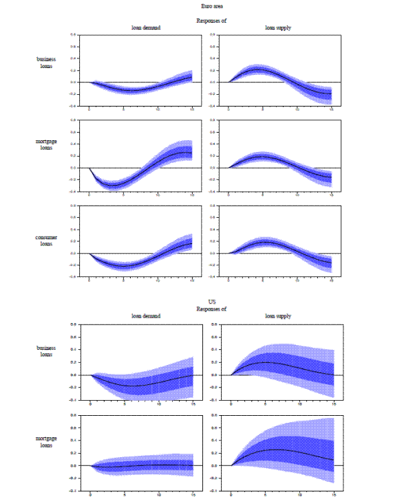
Figure 2A shows the responses of loan demand and supply to a monetary policy shock for all types of loans in the Euro area and in the US. The level and timing of loan supply reduction is significant and similar across different type of loans, whereas there are differences in the responses of loan demand. In the Euro area the reaction of loan demand for mortgages is stronger than for other loans, whereas in the US the response is not statistically significant. This may, at least in part, reflect different institutional characteristics of the mortgage credit markets. For instance, other (non-bank) financial intermediaries are important providers of mortgage loans in the US while this is not the case in (most) Euro area countries; the ratio of fixed to variable loan rates is different in the two economies; conditions for refinancing mortgage loans tend to be more favorable in the US compared to (most) Euro area countries.

These results suggest that the responses to a monetary policy shock of volumes of different kind of loans as reported in den Haan et al (2007) with US data may reflect changes in loan demand more than in loan supply. In the results of den Haan et al (2007), a monetary tightening has a dampening impact only on real estate and consumer loans. Our results, instead, suggest that while the responses to a monetary policy shock across different type of borrowers differ somewhat in size and in timing, the direction of the shock is the same for all type of loans. These differences are likely to reflect the different identification strategy for loan demand and supply that we use in our study.

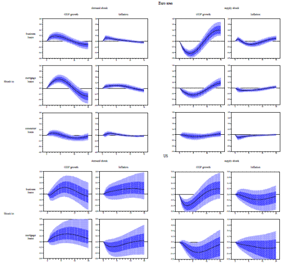
The next step is to analyze the impact of shocks on GDP growth and inflation to the supply of loans. Figure 2B plots the responses of these variables to a tightening of the supply of credit in the Euro area and in the US. A restriction to the supply of loans dampens GDP growth in both economies, with responses to NFC and mortgage loans being more significant than those to consumers' credit, possibly as a consequence of the relatively low importance of this segment of the credit market in most Euro area countries. It is interesting to note that the response of GDP growth is stronger to shocks to NFC loan supply (both in the US and in the Euro area), and mortgage loan demand (Euro area). On the other hand, the impact on inflation is more subdued. In the US this may be related to the high uncertainty surrounding the estimates in this specification. In the euro area a loan supply shock for mortgage and consumer loans dampens inflation almost immediately, whereas a restriction to supply of loans to NFC has a stronger but more delayed impact.

Counterfactual analysis

All in all the results presented so far show that tighter monetary policy restricts bank loan supply to all type of borrowers both in the US and in the Euro area, albeit with some differences in the intensity and in the timing of the impacts. In turn, restrictions to loan supply significantly reduce output growth and inflation. This first evidence, therefore, suggests that a credit channel of monetary policy transmission is active and works through all the lending channels (loans to different borrowers).

As we have done for Model 1, we now quantify the relevance of the credit channel in a framework where all the different classes of borrowers are taken into account. In addition to the questions we have addressed using Model 1, the specification of Model 2 raises two additional issues. First, we can check which borrower category is more relevant for the transmission of monetary policy shocks. Second, as restrictions to loan supply may affect GDP growth and inflation by dampening loan demand (which in turn amplifies the impact on the economy), we can also check the relevance of this indirect channel.

The analysis is carried out using counterfactual experiments. We address the first question by looking at the impact on GDP growth and inflation of a monetary policy shock when the demand and the supply channels for each type of loans as closed down. The results are shown in Figure 2C, where we compare the dynamics of the responses of output growth and inflation to a monetary policy shock (blue line) with counterfactual of responses of the same variables obtained when closing down either the loan supply or the loan demand for each type of loans (black line).26

The figures show that in the Euro area a monetary policy shock has a high impact on GDP growth through mortgage loan demand and supply, and through NFC loan supply, whereas in the US supply (of both business and mortgage loans) seems to matter more than demand. For inflation, both channels (demand and supply) seem to be important across all loan categories. Consumer loans, which do not matter for the transmission of a monetary policy shock to GDP growth, are somewhat relevant for the transmission of the shock to inflation.

Finally, in Figure 2D we check the indirect channel of monetary transmission. The figures show the results of counterfactual experiments where the full-system impact of a credit tightening (shock to supply) on output growth and inflation is compared with the responses of the same variables when closing down the demand channel. The evidence indicates that the tightening of bank loan supply has a significant direct impact on GDP growth, while the indirect effect working through the decline of loan demand is small, especially in the Euro area. At the same time, the effect of the credit channel on inflation depends strongly on the effect that loan supply restrictions have on loan demand especially in the US.

3.2 Firm and household balance-sheet versus bank-lending channel

In this subsection we disentangle the two main sub-channels of the credit channel of the transmission of monetary policy. In particular, we assess the relative importance of the mechanisms of transmission of monetary policy shocks through the balance sheets of banks and borrowers (the bank lending channel and the non-financial borrower balance sheet channel).

To identify these channels we use the rich information provided by the surveys, in particular the answers related to the factors (reasons) inducing banks to change their credit standards to firms and households. We categorize these factors in two broad sets. The pure supply factors are related to the capital and liquidity positions of the banks, their ability to access market financing and to the competitive pressures in the banking sector. These factors affect the ability and incentives of banks to grant loans for a certain quality of the borrowers. Therefore, these factors provide a measure of the importance of the bank lending channel. The current financial crises has emphasized the need to understand deeply these mechanisms in light also of the policies put in place to support the banking sector (see e.g. the forthcoming chapters in the Handbook of Monetary Policy, in particular Adrian and Shin, 2009; Boivin et al., 2009; and Gertler and Kiyotaki, 2009).

The factors related to the borrowers' quality are instead linked to the outlook for firms and households and to the quality of their collateral. Therefore, they are more related to the willingness of banks to lend to borrowers with different risk profiles, hence reflecting different agency problems (see Bernanke, Gertler and Gilchrist 1996 and 1999). We use these factors as indicators of the relevance of the (non-financial borrower) balance sheet channels.

Note that in this context there is an important difference between the two bank lending surveys. In the Euro area BLS there is information on the reasons why banks have changed lending standards both for business and household loans, whereas in the US SLO this information is available only for business loans. As a consequence, we can analyze the household balance-sheet channel only for the Euro area. In the next subsections, we first analyze the firm balance-sheet channel and the bank lending channel for both the US and the Euro area (Model 3). Next, we analyze the household and firm balance-sheet channels for the Euro area and we compare their strength with the bank lending channel (Model 4).

3.2.1 Firm balance-sheet channel and bank lending channel (Model 3)

Figure 3A shows the responses to a monetary policy shock of demand and supply of corporate loans in the Euro area and in the US. The response of loan supply is further disentangled between the effect working through the bank lending channel and the firm balance-sheet channel. In the Euro area a monetary tightening reduces loan supply through the bank lending channel (pure supply, i.e. banks tighten the standards because of bank balance sheet constraints and competitive pressures) and the firm balance-sheet channel (borrower's quality, i.e., banks tighten their standards because of worse firm risk, outlook and collateral). The responses are significantly estimated and show a comparable positive impact (tightened credit standards) peaking at around four to five quarters. In the US, responses are subject to a higher degree of uncertainty. Nevertheless the estimates show that the impact of a monetary tightening affects significantly the bank lending channel at 68%, while the response of factors related to firms' quality is generally not significant. There are also some differences in the timing of responses between the two economies. The impacts in the Euro area peak at slightly longer horizons than in the US, though qualitatively the dynamic of the responses is similar, with pure supply peaking slightly earlier than firm's quality in both economies.

Figure 3B plots the responses of GDP growth and inflation to a shock to bank pure supply and firms' quality factors for the Euro area and for the US. In the Euro area the two loan supply channels are significantly affecting GDP growth and - to a lesser extent - inflation, with a comparable lag: the responses of output growth peak between three and four quarters, whereas the responses of inflation reach a maximum approximately after five to six quarters. In terms of magnitude, the impact on GDP growth and inflation of shocks to the pure supply (bank lending) channel is on average twice as big as the effect of shocks to firm's quality.

In the US only shocks to the firm's quality (firm channel) have a significant impact on GDP, while the responses to the bank pure supply factors are not significant. This difference between the responses in the Euro area and in the US may reflect differences in the banking structure of the two economies. In particular, the corporate sector in the US is less reliant on bank loans, and thus restrictions of firms' access to bank credit may have a lower impact on GDP growth (see Allen et al., 2004).

Overall, these results confirm that both a firm balance-sheet and a bank-lending channel play a significant role in the transmission mechanism in the Euro area and in the US at least concerning the impact on GDP growth. To further investigate and better quantify the relative importance of the two channels, we use counterfactual experiments, similar to the ones performed in the previous sections. We analyze which factors amplify more the responses of output growth and inflation to a monetary policy shock. Figure 3C shows the results of this analysis. Note that in the Euro area the effect on GDP growth of a monetary policy shock is amplified more by the mechanisms of the bank lending channel (pure supply factors) compared to the effect working through firm's quality (balance-sheet channel) or through loan demand; the effect on inflation is instead higher through the borrower's quality and the loan demand channel. On the other hand, in the US the firm balance-sheet and loan demand channels are more important both for GDP and inflation.

The results on the bank lending channel give support to the somewhat different policies that were put in place during the current crisis. In the US the central bank has implemented policies directed to support both banks and firms (e.g. in commercial paper), whereas in the Euro area interventions have mainly targeted banks (e.g. the credit enhancement of the ECB).

3.2.2 All subchannels including the household balance-sheet channel (Model 4)

In the last VAR specification considered, we include loan demand, pure supply and borrower's quality factors for loans to all borrowers: firms, mortgages and consumer loans. This specification (Model 4 in section 3) is used to analyze the importance of the transmission channels working through the balance sheet of banks and non-financial borrowers (banks, firms and households, respectively). As observed earlier, we can do this analysis only for the Euro area since we have information from the BLS on whether changes in lending standards for households (either for house purchase or for consumption) are due to changes in bank pure supply factors (bank capital, liquidity and competition) or in households' quality (outlook and risk of collateral).

Figure 4A shows the responses of loan demand and loan supply to firms and households to a monetary tightening through the bank lending and the non-financial borrower balance-sheet channels. A monetary tightening reduces loan supply through the bank lending channel (pure supply) and also through the firm and household balance-sheet channels. The responses are significant and show a comparable positive impact (tightened credit standards) with peaks around four to five quarters and similar magnitudes. The responses are broadly similar across type of loans.

Figure 4B shows the responses of GDP growth and inflation to shocks to loan supply for firms and households (through the bank lending and the firm/household balance-sheet channels). Concerning the impact on GDP growth, the results relative to the firm bank lending channel (i.e. pure bank supply restrictions to firms) are similar to what shown in Figures 3A to 3C. The supply for consumer loans is not very relevant. For loans for house purchase the household balance-sheet channel is more important than the (household) bank lending channel. This implies that shocks to the supply of mortgages are relevant for GDP growth because of mechanisms working through households' quality channels, consistently with Bernanke et al. (1996), who point out that households may be more financially constrained due to human capital inalienability (see also Hart and Moore 1994), implying that monetary policy has stronger effects through household loans.

The results for inflation suggest also a difference across lending markets. The impact on inflation is more significant for business loans through the bank lending channel. On the other hand, credit to households affects inflation by channels working through borrower's quality and demand. These results may have interesting policy implications. Policies aimed at sustaining aggregate demand and improving balance sheet of non-financial borrowers may be more effective in supporting the credit markets for mortgages. However, they may also have more impact on inflation.

To assess the relevance of the different channels of transmission of credit supply we run a counterfactual analysis as done in the previous sections (Figure 4C). All in all the results confirm that in terms of impact on GDP growth, the bank lending channel is more important for firms and the household balance-sheet channel is more important for mortgage loans. On the other hand, demand for business and consumer loans and household balance sheet channel for house purchase generates more significant effects on inflation.

3.3 The financial crisis

In this section, the VAR methodology is used to analyze the relative importance of different shocks during the financial and economic crises and to shed some light on the relationship between the financial sector and the macroeconomy (in crises periods). Specifically, we assess the role played by the impairment of the financial sector and the consequent credit crunch on the economy and also the effectiveness of monetary policy interventions - namely overnight interest rates cuts.

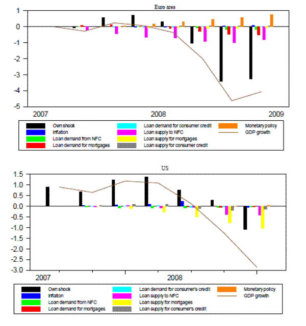
We report in Figure 5A a shock decomposition for both economies using the specification of Model 2. The bars in the charts represent the effects at time t of innovations to other variables which explain movements in the variables of interest.27

In the Euro area, apart from the own shocks, changes in GDP growth were mostly affected by restrictions of bank loan supply to business loans. Therefore, the impairment of the financial sector due to the crisis seems to have affected primarily business loans (which on average have shorter maturity) and this, in turn, had a negative impact on GDP growth. In the last quarters also the decline in demand for loans for house purchase reduced significantly output growth. This is consistent with a deteriorating outlook for the real economy which dampens demand for loans from the household sector. At the same time, monetary policy shocks (primarily policy rate cuts but also indirectly the full allotment policy) have supported GDP growth, which presumably would have been lower if an accommodative monetary policy stance had not been put in place.28 The policies aimed at sustaining bank's liquidity may have partly relaxed the liquidity position of banks and been conducive to less tight lending standards than otherwise.

The same analysis for the US yields qualitatively different results. Apart from "own shocks", restrictions to the supply of mortgage loans are among the most important shocks to explain changes in GDP growth over the period 2007Q3-2009Q2. Restrictions to the supply of business loans are also important. At the same time, monetary policy shocks play an almost neutral role. These results may be due to differences in the structure of the financial system between the US and the Euro area, but also to our identification strategy. Concerning the latter, the Fed has engaged in a diversified and multifaceted strategy of non-conventional monetary policy measures, aimed at supporting not only the financial sector (by increasing the number of financial institutions, and the quality of collateral, which could draw on central bank liquidity) but also the corporate sector, for example by buying commercial papers. This may partly explain why restrictions to business loans play a minor role than in the Euro area, and why shocks to the Fed funds rate may not be able to capture fully the importance of a monetary policy shock.

Finally, we investigate the relative importance of all the channels of loan supply. Figure 5B shows the shock decomposition using Model 4 for the Euro area (no comparable data are available for the US). Apart from the own shock, the most important shock affecting negatively GDP growth are loan supply restrictions to firms due to banks' balance-sheet weaknesses, i.e. the bank lending channel. This suggests that problems in bank capital and liquidity significantly reduced GDP growth before and during the crisis, and hence that the financial crisis has contributed to generate the economic recession.

4 Concluding remarks

Most developed countries around the world have experienced the worst banking crisis of the post-war period. The global economic recession that has followed also appears to be the most severe of this era. The role played by the banking sector in affecting the macroeconomy, in particular through the supply of credit to the private sector, has become a central issue of concerns for academics and policy makers alike. The issues of interest revolve around three main questions: (i) whether problems to liquidity and capital position of banks affect their lending decisions; (ii) whether this, in turn, has an impact on aggregate output and inflation; and (iii) whether and how monetary policy impulses are transmitted to the rest of the economy, in particular through the banking sector. Our objective in this paper is to test the credit channel of monetary transmission and to explore the dynamics of credit during the current crisis.

There are two key identification problems that the empirical literature on the credit channel has to face: (i) disentangling of loan demand and loan supply; (ii) the separation of the mechanisms related to the bank lending and the (non-financial borrower) balance-sheet channels. Our identification strategy is based on the use of the answers from the confidential Euro area Bank Lending Survey and the U.S. Senior Loan Officer Survey. National central banks of the Eurosystem and regional Feds carry out these surveys to gather quarterly information on the loan demand that banks receive and on the lending standards that banks apply to firms and households, including the factors affecting banks' decisions to change their lending standards.

Our results suggest that the credit channel is broadly operational for all type of channels and loans. Moreover, the impact of a monetary policy shock on GDP growth is higher through loan supply than through loan demand, whereas the latter affects more inflation. In addition, the bank lending channel amplifies the effect on GDP growth more than the firm balance-sheet channel both in the Euro area and in the US. At the same time, the firm balance-sheet channel and the loan demand channel have a larger impact on inflation (at least in the Euro area). Finally, the household balance-sheet channel is more important than the bank lending channel for mortgage loans.

In the last part of the paper we also address the important question whether the strong evidence we find for the credit channel is due to our identification of loan demand and supply or to the current crisis. A shock decomposition of GDP growth during the crisis period suggests that a key factor is the restriction of loan supply to businesses due to bank liquidity and solvency problems in the Euro area. In the U.S., restrictions to the supply of mortgage loans are among the most important shocks to explain changes in GDP growth during the crisis period. Finally, our analysis suggests that the policies of central banks based on very low interest rates and measures aimed at relaxing banks' balance-sheets constraints have been providing a significant support to the real economy.

Bibliography

Allen F, Chui, M. and Maddaloni, A.,
"Financial Systems in Europe, the USA and Asia," Oxford Review of Economic Policy, 2004, 20(4), 490-508.
Adrian T. and H. S. Shin,
"Financial Intermediaries and Monetary Economics," Handbook of Monetary Economics, 2009, forthcoming.
Altavilla C., and M. Ciccarelli,
"The effects of monetary policy on unemployment dynamics under model uncertainty: Evidence from the US and the Euro area," Journal of Money, Credit and Banking, 2009, 41, 1265-1300.
Angeloni I., Kashyap, A. and B. Mojon,
Monetary Policy Transmission in the Euro area, 2003.
Angeloni I. and E. Faia, 2009,
"A Tale of Two Policies: Prudential Regulation and Monetary Policy with Fragile Banks," mimeo.
Berg, J.; van Rixtel, A.; Ferrando, A.; de Bondt, G.; Scopel, S.
"The bank lending survey for the Euro area" Occasional Paper, European Central Bank, Frankfurt, 2005
Bernanke B. S.
"The Financial Accelerator and the Credit Channel." Remarks - Credit Channel of Monetary Policy in the Twenty-first Century, Board of Governors of the US Federal Reserve System, Washington DC, 2007.
Bernanke B. S. and Blinder, A. S.
"The Federal Funds Rate and the Channels of Monetary Transmission." American Economic Review, 1992, 82(4), pp. 901-21.

"Money Credit and Aggregate Demand." American Economic Review, 1988, 82, pp. 901-21.
Bernanke B. S., and Gertler, M.
"Banking in General Equilibrium," in W. Barnett and K. Singleton (eds.), New Approaches to Monetary Economics (Cambridge: Cambridge University Press, 1987).

"Agency Costs Net Worth, and Business Fluctuations," American Economic Review, 1989, 79(1), pp. 14-31.

"Inside the Black Box: The Credit Channel of Monetary Policy Transmission." Journal of Economic Perspectives, 1995, 9(4), pp. 27-48.
Bernanke B. S.; Gertler, M. and Gilchrist, S.
"The Financial Accelerator and the Flight to Quality." Review of Economics and Statistics, 1996, 78(1), pp. 1-15.

"The Financial Accelerator in a Quantitative Business Cycle Framework" in J. Taylor and M. Woodford, eds., Handbook of Macroeconomics. Amsterdam: Elsevier, 1999, 1341-93.
Bernanke B. S. and Kuttner, K. N.
"What Explains the Stock Market's Reaction to Federal Reserve Policy?" Journal of Finance, 2005, 60(3), pp. 1221-58.
Bernanke B. S., and I. Mihov, (1998).
"Measuring Monetary Policy." Quarterly Journal of Monetary Policy CXIII, 869-902.
Bernanke B. S., 2009a,
"The Crisis and the Economic Policy Response," Mimeo.
Black L. K. and Rosen, R. J.
"The Effect of Monetary Policy on the Availability of Credit: How the Credit Channel Works." Mimeo, Board of Governors of the Federal Reserve System, Washington DC, 2008.
Boivin J., M. Kiley and F. Mishkin, 2009,
"How Has the Monetary Transmission Mechanism Evolved Over Time?" forthcoming in the Handbook of Monetary Economics.
Camacho M., Perez-Quiros, G. and Saiz, L,
"Are European business cycles close enough to be just one?," Journal of Economic Dynamics and Control, 2006, Elsevier, vol. 30(9-10), pages 1687-1706.
Christiano L. J.; Eichenbaum, M. and Evans, C.
"The Effects of Monetary Policy Shocks: Evidence from the Flow of Funds." Review of Economics and Statistics, 1996, 78(1), pp. 16-34.
Christiano L.J., Eichenbaum, M., Evans, C.L., 1999.
Monetary policy shocks: what have we learned and to what end? In: Taylor, J.B., Woodford, M. (Eds.), Handbook of Macroeconomics. North-Holland, Amsterdam.
Den Haan W. J.; Sumner, S. and Yamashiro, G.
"Bank Loan Portfolios and the Monetary Transmission Mechanism." Journal of Monetary Economics, 2007, pp. Forthcoming.
Diamond D. W., and R. G. Rajan, 2000,
A Theory of Bank Capital, Journal of Finance 55, 2431-2465.
Diamond D. W., and G. R. Rajan, 2001,
Liquidity Risk, Liquidity Creation, and Financial Fragility: A Theory of Banking, Journal of Political Economy 109, 287-327.
Diamond D. W. and Rajan, R. G.
"Money in a Theory of Banking." American Economic Review, 2006, 96(1), pp. 30-53.
Diamond D. W. and R. Rajan, 2009,
"Illiquidity and Interest Rate Policy," mimeo.
Doan T.,
"Understanding the Historical Decomposition", mimeo ESTIMA, June, 2009.
European Central Bank
"Recent Developments in the Balance Sheets of the Eurosystem, the Federal Reserve System and the Bank of Japan." ECB Monthly Bulletin, 2008, October, pp. 81-94.
Freixas X., and J. C. Rochet, 2008.
Microeconomics of Banking (MIT Press, Cambridge MA).
Friedman B., and Kuttner, K.
"Economic Activity and the Short term Credit Markets: An Analysis of Prices and Quantities," Brookings Papers on Economic Activity (1993:2), 193-284.
Gertler Mark,
"Financial Structure and Aggregate
Fostel A. and Geanakoplos J., 2009,
"Leverage Cycles and the Anxious Economy," American Economic Review.
Gerdesmeier D., Mongelli F. and Roffia B.,
"The Eurosystem, the U.S. Federal Reserve and the Bank of Japan: Similarities and Differences," Journal of Money, Credit and Banking, 2007, Vol. 39, No. 7, pp. 1785-1819.
Gertler M. and Gilchrist, S.
"Monetary Policy, Business Cycles, and the Behavior of Small Manufacturing Firms." Quarterly Journal of Economics, 1994, 109, pp. 309-40.

"The Role of Credit Market Imperfections in the Monetary Transmission Mechanism: Arguments and Evidence." Scandinavian Journal of Economics, 1993, 95, pp. 43-64.
Gertler M. and P. Karadi, 2009,
"A Model of Unconventional Monetary Policy," mimeo.
Gertler M. and Kiyotaki, N., 2009,
"Financial Intermediation and Credit Policy in Business Cycle Analysis," forthcoming in the Handbook of Monetary Economics.
Giannone D., M. Lenza, and L. Reichlin, 2008,
Monetary analysis with disaggregated variables, ECB Mimeo.
Hart Oliver and John Moore, 1994,
"A Theory of Debt Based on the Inalienability of Human Capital", Quarterly Journal of Economics, 109(4), 841-79.
Hartmann P., Maddaloni, A. and Manganelli, S.
"The Euro-Area Financial System: Structure, Integration, and Policy Initiatives," Oxford Review of Economic Policy, 2003, Vol. 19, No. 1, pp. 180- 213.
Hempell, H.S., Köhler-Ulbrich P. and S. Sauer,
"Information from the Euro area bank lending survey," ECB Occasional Paper, 2009, forthcoming.
Ioannidou V. P., S. Ongena, and J.-L. Peydró, 2009,
Monetary Policy, Risk-Taking and Pricing: Evidence from a Quasi-Natural Experiment, (CentER - Tilburg University / European Central Bank, Tilburg), Mimeo.
Jiménez G., S. Ongena, J.-L. Peydró, and J. Saurina, 2008,
Hazardous Times for Monetary Policy: What Do Twenty-Three Million Bank Loans Say about the Effects of Monetary Policy on Credit Risk?, (Banco de España, Madrid), Documentos de Trabajo 833.
Jiménez G., S. Ongena, J.-L. Peydró, and J. Saurina,
"Credit Availability: Identifying Balance-Sheet Channels with Loan Applications and Granted Loans," ECB Mimeo, 2009.
Kadiyala K. R. and S. Karlsson,
Numerical Methods for Estimation and Inference in Bayesian VAR models, Journal of Applied Econometrics, 12(2), 99-132, 1997.
Kashyap A. K. and Stein, J. C.
"What Do a Million Observations on Banks Say About the Transmission of Monetary Policy?" American Economic Review, 2000, 90(3), pp. 407-28.
King R., and Plosser, C.
"Money, Credit, and Prices in a Real Business Cycle," American Economic Review 74 (June, 1984), 363-380.
Kiyotaki Nobuhiro,
"Multiple Expectational Equilibria Under Monopolistic
Kiyotaki Nobuhiro and John Moore, 1997,
"Credit Cycles," Journal of Political Economy.
Kiyotaki Nobuhiro and John Moore, 2008,
"Liquidity, Business Cycles and Monetary Policy," mimeo.
Khwaja A., and A. Mian, 2008,
Tracing the Impact of Bank Liquidity Shocks: Evidence from an Emerging Market, American Economic Review Forthcoming.
Lang William W., and Leonard I. Nakamura, 1995,
'Flight to Quality' in Banking and Economic Activity, Journal of Monetary Economics 36, 145-164.
Lown C.; and Morgan, D. P.,
"The Credit Cycle and the Business Cycle: New Findings Using the "Lost" Series on Commercial Credit Standards," Proceedings, Federal Reserve Bank of Chicago, issue May, 2002, pp. 282-307.
Lown C.; and Morgan, D. P.,
"The Credit Cycle and the Business Cycle: New Findings Using the Loan Officer Opinion Survey," Journal of Money, Credit and Banking, 2006, Vol. 38, No.6, September, pp. 1575-1597.
Lown C.; Morgan, D. P., and Rohatgi, S.
"Listening to Loan Officers: the Impact of Commercial Credit Standards on Lending and Output," Economic Policy Review, Federal Reserve Bank of New York, issue July, 2000, pp. 1-16.
Maddaloni, A. and J.-L. Peydró,
"Bank Risk-Taking, Securitization, Supervision, and Low Interest Rates: Evidence from Lending Standards, paper presented at the RFS-Yale Conference The Financial Crisis, 2009.
Matsuyama K.
"Credit Traps and Credit Cycles." American Economic Review, 2007, 97(1), pp. 503-16.
Mishkin F. S.,
"What Depressed the Consumer? The Household Balance Sheet and the, 1973-75 Recession," Brookings Papers on Economic Activity (1977:1),123-164.

"The Household Balance Sheet and the Great Depression," Journal of Economic History 38 (Dec., 1978),918-937.
Peek J., and E. Rosengren, (1995)
The Capital Crunch: Neither a Borrower nor a Lender Be Source: Journal of Money, Credit and Banking, Vol. 27, No. 3 (Aug., 1995), pp. 625-638.
Peek J. and E. S. Rosengren, (1995).
"Is bank lending important for the transmission of monetary policy? An overview," New England Economic Review, Federal Reserve Bank of Boston, issue Nov, pages 3-11.
Peek J., and E. S. Rosengren, (1997)
The International Transmission of Financial Shocks: The Case of Japan. The American Economic Review, Vol. 87, No. 4 (Sep., 1997), pp. 495-505.
Peek J. and E. S. Rosengren (forthcoming)
"The Role of Banks in the Transmission of Monetary Policy", in The Oxford Handbook of Banking, A. Berger, P. Molyneux, and J. Wilson, eds. (Oxford: Oxford University Press).
Ramey V. A., 1993.
How Important is the Credit Channel in the Transmission of Monetary Policy?," NBER Working Papers 4285.
Romer C.and D. Romer
"New Evidence on the Monetary Transmission Mechanism" Brookings Papers on Economic Activity, 1990, No. 1, 149-198.
Rigobon R. and Sack, B.
"The Impact of Monetary Policy on Asset Prices." Journal of Monetary Economics, 2004, 51(8), pp. 1553-75.
Sauer, S., 2009,
"The Euro area Bank Lending Survey - A Review of Six Years of Experience", Revue bancaire et financière, forthcoming.
Stein Jeremy C., 1998,
An Adverse-Selection Model of Bank Asset and Liability Management with Implications for the Transmission of Monetary Policy, RAND Journal of Economics 29, 466-486.
Stiglitz J. E.
"Information and the Change in the Paradigm in Economics." Prize Lecture, Nobel Foundation, Stockholm, 2001.
Stiglitz J. E. and Greenwald, B.
Towards a New Paradigm in Monetary Economics. Cambridge University Press, 2003.
Stiglitz J. E. and Weiss, A.
"Credit Rationing in Markets with Imperfect Information." American Economic Review, 1981, 71, pp. 393-410.


5 Appendix

5.1 Bank Lending Survey (BLS)

Table 5.1.1. Questions on changes to credit standards and to loan demand

Table 5.1.1a. Supply of loans

Question Variable Definition
Over the past three months, how have your bank's credit standards as applied to the approval of loans or credit lines to enterprises changed? (Q1) Net percentage of banks reporting a tightening of credit standards Difference between the sum of banks answering "tightened considerably" and "tightened somewhat" and the sum of banks answering "eased somewhat"and "eased considerably" in percentage of the total number of banks.
Over the past three months, how have your bank's credit standards as applied to the approval of loans to households changed? (Q8) Net percentage of banks reporting a tightening of credit standards Difference between the sum of banks answering "tightened considerably" and "tightened somewhat" and the sum of banks answering "eased somewhat"and "eased considerably" in percentage of the total number of banks.


Table 5.1.1b. Demand of loans

Question Variable Definition
Over the past three months, how has the demand for loans or credit lines to enterprises changed at your bank; apart from normal seasonal fluctuation? (Q4) Net percentage of banks reporting an increase of the demand for loans Difference between the sum of banks answering "increased considerably" and "increased somewhat" and the sum of banks answering "decreased somewhat" and "decreased considerably" in percentage of the total number of banks.
Over the past three months, how has the demand for loans or credit lines to households changed at your bank; apart from normal seasonal fluctuation? (Q13) Net percentage of banks reporting an increase of the demand for loans Difference between the sum of banks answering "increased considerably" and "increased somewhat" and the sum of banks answering "decreased somewhat" and "decreased considerably" in percentage of the total number of banks.


Table 5.1.2. Questions on factors affecting changes in credit standards

Question Factors Variable Definition
Q2 Over the past three months, how have the dollowing factors affected your bank's credit standards as applied to the approval of loans or credit lines to enterprises? A. Costs of funds and balance sheet constraints

Costs related to your bank's capital position

Your bank's ability to access market financing

Your bank's liquidity position

B. Pressure from competition

Competition from other banks

Competition from non-banks

Competition from market financing

C. Perception of risk

Expectations regarding general economic activity

Industry or firm-specific outlook

Risk on the collarteral demanded

Net percentage of banks reporting that each of these factors has contributed to the tightening of standards to enterprises.

Pure supply = average of the responses to A and B;

Borrower quality = average of the responses to C

Difference between the sum of the banks answering "contributed considerably to tightening" and "contributed somewhat to tightening" and the sum of the banks answering "contributed somewhat to easing" and "contributed considerably to easing" in percentage of the total number of banks.
Q9 Over the past three months, how have the following factors affected your bank's credit standards as applied to the approval of loans to households for house purchase? A. Costs of funds and balance sheet constaints

B. Pressure from competition

Competition from other banks

Competition from non-banks

C. Perception of risk

Expectations regarding general economic activity

Housing market prospects

Net percentage of banks reporting that each of these factors has contributed to the tightening of standards to enterprises

Pure supply = average of the responses to A and B;

Borrower quality = average of the responses to C

Difference between the sum of the banks answering "contributed considerably to tightening" and "contributed somewhat to tightening" and the sum of the banks answering "contributed somewhat to easing" and "contributed considerably to easing" in percentage of the total number of banks.
Q11 Over the past three months, how have the following factors affected your bank's credit standards as applied to the approval of consumer credit and other lending to households? A. Costs of funds and balance sheet constraints

B. Pressure from competition

Competition from other banks

Competition from non-banks

C. Perception of risk

Expectations regarding general economic activity

Creditworthiness of consumers

Risk on the collateral demanded

Net percentage of banks reporting that each of these factors has contributed to the tightening of standards to enterprises.

Pure supply = average of the responses to A and B;

Borrower quality = average of the responses to C

Difference between the sum of the banks answering "contributed considerably to tightening" and "contributed somewhat to tightening" and the sum of the banks answering "contributed somewhat to easing" and "contributed considerably to easing" in percentage of the total number of banks.
Note: Q* indicates the number of the question in the survey
Source: ECB, http://www.ecb.europa.eu/stats/money/surveys/lend/html/index.en.html

5.2. Senior Loan Officer Survey (SLO)

5.2.1. Questions on changes to credit standards and to loan demand

Table 5.2.1a. Supply of loans

Question Variable Definition
Over the past three months, how have your bank's credit standards for approving applications for C&I loans or credit lines - other than those to be used to finance mergers and acquisitions - to large and middle-market firms changed? Q1 Net percentage of banks reporting a tightened of credit standards Difference between the sum of banks answering "tightened considerably" and "tightened somewhat" and the sum of banks answering "eased somewhat" and "eased considerably" in percentage of the total number of banks
Over the past three months, how have your bank's credit standards for approving applications from individuals for mortage loans to purchase homes changed? (Q9) Net percentage of banks reporting a tightened of credit standards Difference between the sum of banks answering "tightened considerably" and "tightened somewhat" and the sum of banks answering "eased somewhat" and "eased considerably" in percentage of the total number of banks
Over the past three months, how have your bank's credit standards for approving applications for consumer loans other than credit card loans changed? (Q15) Net percentage of banks reporting a tightened of credit standards Difference between the sum of banks answering "tightened considerably" and "tightened somewhat" and the sum of banks answering "eased somewhat" and "eased considerably" in percentage of the total number of banks


Table 5.2.1b. Demand for loans

Question Variable Definition
Apart from normal seasonal variation, how has demand for C&I loans changed over the past three months? (Q4) Net percentage of banks reporting an increased of the demand for loans. Difference between the sum of banks answering "increased considerably" and "increased somewhat" and the sum of banks answering "decreased somewhat" and "decreased considerably" in percentage of the total number of banks.
Apart from normal seasonal variation, how has demand for mortage to purchase homes changed over the past three months? (Q10) Net percentage of banks reporting an increased of the demand for loans. Difference between the sum of banks answering "increased considerably" and "increased somewhat" and the sum of banks answering "decreased somewhat" and "decreased considerably" in percentage of the total number of banks.
Apart from normal seasonal variation, how has demand for consumer loans of all types changed over the past three months? (Q18) Net percentage of banks reporting an increased of the demand for loans. Difference between the sum of banks answering "increased considerably" and "increased somewhat" and the sum of banks answering "decreased somewhat" and "decreased considerably" in percentage of the total number of banks.

Note: Q* indicates the number of the question in the survey
Source: Federal Reserve Board, http://www.federalreserve.gov/boarddocs/snloansurvey/

5.2.2. Questions on factors affecting changes in credit standards

Question Factors Variable
Q3 if your bank has tightened or eased its credit standards or its terms for C&I loans or credit lines over the past three months, how important have been the following possible reasons for the change? A. Current or expected capital position

B. Economic outlook and its uncertainty

C. Industry specific problems

Pure supply = responses to A

Borrower quality = average of the responses to B and C

Note: Q* indicates the number of the question in the survey
Source: Federal Reserve Board, http://www.federalreserve.gov/boarddocs/snloansurvey/

Figure 1A: Responses of demand and supply of
business loans to a monetary policy shock

Figure 1: Responses of demand and supply of business loans to a monetary policy shock. This figure contains four line plots showing the response of demand for loans and supply of loans to a one standard deviation shock to the overnight rate for the Euro area and the US. The 68% Bayesian credible interval is dark blue, and the 90% Bayesian credible interval is light blue.  The y-axes have limits of -0.4 to 0.4, and the x-axes have limits of 0 to 15.  
In the first panel which is Euro area's demand for loans, the line starts at (0,0) and gently dips down reaching the trough of about -0.1% at about 5, then gradually rises above the y-value of 0 at around 12, so it is a gentle U-shape.
In the second panel which is Euro area's supply of loans, the line starts at (0,0) and quickly goes up to reach 0.2 at around 4, before decreasing in value again, crossing the 0 y-value and ending at about -1.5 at 15.
In the third panel, which is the US's demand for loans, the lines starts at (0,0) and gently slopes downward before reaching the lowest point a value of almost -0.2 at around 5, before sloping back upwards again and crossing the y-value of 0 at around 11 or 12, and ends with a value of about 0.1 at 15.
In the fourth panel, which is the US's supply of loans, the line starts at (0,0) and gently slopes upward, reaching a maximum of about 0.1 at around 4  before decreasing again, crossing the y-value of 0 at around 9 and then flattening out as it ends with a value of -0.1 at 15.
Note: These graphs plot the responses of loan demand and loan supply to a one-standard deviation shock to the overnight rate. Only business loans (loans to non-financial corporations) are considered. Responses of the series are normalised and divided by their innovation variances so that all responses to a shock are comparable on a single scale. The median response is shown along with 68 (dark blue) and 90 (light blue) percent Bayesian credible intervals, computed by estimating the VAR with a flat prior on the parameters and assuming normality of the error terms. The graphs on the first row refer to the Euro area, while the second row shows the responses for the United States (US). The panel VAR for the Euro Area is estimated assuming fixed effects, slope homogeneity and the country identification strategy as explained in Section 3. The specification of the VAR includes 5 variables: GDP growth, inflation, total demand of loans from NFC and total supply of loans to NFC (see specification of MODEL 1 in Section 3.5.) See Section 3 and Appendix for a detailed definition of the variables.

Figure 1B: Responses of GDP growth and inflation to shocks to demand and supply of business loans

Figure 2: Responses of GDP growth and inflation to shocks to demand and supply of business loans. This figure contains eight line plots showing the response of GDP growth and inflation to a one standard deviation shock to demand and supply of business loans for the Euro Area and the US. The 68% Bayesian credible interval is dark blue, and the 90% Bayesian credible interval is light blue.  The y-axes have limits of -1 to 1, and the x-axes have limits of 0 to 15.  
In the first panel which is Euro area's response of GDP growth to a shock to demand for loans, the line starts at (0,0) before increasing and peaking at a y-value of about 0.25 at around 3, and then gradually sloping down, crossing the y-value of 0 at around 11 and ending just slightly below 0 at 15.
In the second panel which is Euro area's response of GDP growth to a shock to supply of loans, the line starts at (0,0) before decreasing and reaching at trough at a y-value of -0.50 at about 3.5. It then increases, crossing the y-value of 0 at around 9 and ending at about 0.25 at 15.
In the third panel which is Euro area's response of inflation to a shock to demand for loans, the line starts at (0,0) before increasing and peaking at a y-value of about 0.12 at around 2, and then very gradually sloping down, crossing the y-value of 0 at around 13 and ending just very slightly below 0 at 15.
In the fourth panel which is Euro area's response of inflation to a shock to supply of loans, the line starts at (0,0) before increasing very slightly to reach a y-value of just above 0 at about 1 before gradually sloping down to reach a trough of about -0.12 at about 6. It then gradually slopes upward again, crossing the y-value of 0 at around 11 and ending at about 0.10 at 15.
In the fifth panel which is the US's response of GDP growth to a shock to demand for loans, the line starts at (0,0) before dipping down briefly to -0.12 at about 1 and then increasing again, crossing the y-value of 0 at about 3 and peaking at a y-value of about 0.18 at around 8, and then sloping down and ending at 0 at 15.
In the sixth panel which is the US's response of GDP growth to a shock to supply of loans, the line starts at (0,0) before rapidly decreasing and reaching at trough at a y-value of -0.70 at about 4. It then increases, crossing the y-value of 0 at around 10 and ending at about 0.25 at 15.
In the seventh panel which is the US's response of inflation to a shock to demand for loans, the line starts at (0,0) before very gradually increasing to end at about 0.12 at 15.
In the eighth panel which the US's response of inflation to a shock to supply of loans, the line starts at (0,0) before staying flat to 1 and then decreasing to a trough of -0.30 at about 9, and then increasing again to end at -0.20 at 15.
Note: These graphs plot the responses of GDP grwoth and inflation to a one-standard deviation shock to demand for and supply of loans. Only business loans (loans to non-financial corporations) are considered. Responses of the series are normalised and divided by their innovation variances so that all responses to a shock are comparable on a single scale. The median response is shown along with 68 (dark blue) and 90 (light blue) percent Bayesian credible intervals, computed by estimating the VAR with a flat prior on the parameters and assuming normality of the error terms. The graphs on the first two rows refer to the Euro area, while the others show the responses for the United States (US). The panel VAR for the Euro Area is estimated assuming fixed effects, slope homogeneity and the country identification strategy as explained in Section 3. The specification of the VAR includes 5 variables: GDP growth, inflation, total demand of loans from NFC and total supply of loans to NFC (see specification of MODEL 1 in Section 3.5.) See Section 3 and Appendix for a detailed definition of the variables.

Figure 1C: Counterfactual analysis. Responses of GDP growth and inflation to a monetary policy shock with and without credit channels (for business loans)
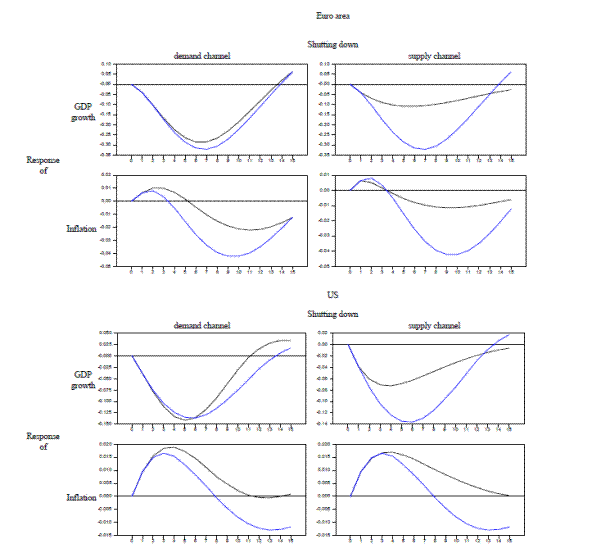
Figure 1C: Counterfactual analysis. Responses of GDP growth and inflation to a monetary policy shock with and without credit channels (for business loans). This figure contains eight line plots (each with two lines) showing the response of GDP growth and inflation to a one standard deviation monetary policy shock for the Euro Area and the US. The x-axes have limits of 0 to 15, and the y-axes limits vary for each panel. The black lines are computed from a system where the supply or demand channel has been closed down, and the blue lines are the responses for the system where all the channels are active.
In the first panel, which is the Euro area's response of GDP growth to a shutting down in the demand channel, the y-axes go from -0.35 to 0.10 and the two lines start at (0,0) before decreasing, with the blue line decreasing at a slightly faster rate than the black line. They both reach their low points of -0.33 (for blue line) and -0.27 (for the black line) at around 6.5 before increasing. The blue line increases slightly faster than the black line, and the two cross the y-value of 0 between 13 and 14, and eventually converge at a y-value of 0.05 at 15.
In the second panel, which is the Euro area's response of GDP growth to a shutting down in the supply channel, the y-axes go from -0.35 to 0.10 and the two lines start at (0,0). First they decrease, with the blue line staying with the black line until -0.05 at 1 and then rapidly separating and becoming more negative. The blue lines reaches a trough of -0.30 at 7 and the black line reaches a shallow trough of about -0.10 at 5.  The blue line increases rapidly from its low-point and crosses the black line at a y-value of -0.05 at about 13. The blue line crosses the y-value of 0 at about 14 and ends at 0.05, whereas the black line ends at -0.025 at 15.
In the third panel, which is the Euro area's response of inflation to a shutting down in the demand channel, the y-axes go from -0.05 to 0.02 and the two lines start at (0,0). First they increase, with the black line increasing at fast rate than the blue line. The black lines reach a peak of 0.01 at 2.5 and the blue lines reaches a peak of slightly below 0.01 at 2. Both lines then slope downward, with the blue line having a steeper slope. The black line crosses the y-value of 0 at about 5.5 and the blue line crosses at 3. The blue line reaches a low point of -0.04 about 9.5 before sloping back up, and the black line reaches a low-point of -0.02 at about 11. The two lines meet on the upslope at a value of -0.015 at 15.
In the fourth panel, which is the Euro area's response of inflation to a shutting down in the supply channel, the y-axes go from -0.05 to 0.01 and the two lines start at (0,0). First the two lines increase together until 0.05 at 1, but then the black line decreases while the blue line increases until 0.008 at 2 before coming down again. However, both lines cross the y-value of 0 at 4. The blue line decreases much more rapidly, reaching a low point of -0.04 at 9.5, while the black line reaches a shallow low point at -0.01 at about 9.5.  The black line ends on the upslope at -0.07 at 15 and the blue line ends at -0.012 at 15.
In the fifth panel, which is the US's response of GDP growth to a shutting down in the demand channel, the y-axes go from -0.15 to 0.05 and the two lines start at (0,0) before decreasing, with the black line decreasing at a slightly faster rate than the blue line. They both reach their low points of -0.13 at 6 (for the blue line) and -0.14 at 5 (for the black line) before increasing. The black line increases slightly faster than the blue line and crosses the y-value of 0 at 11, ending at 0.030. The blue line crosses the y-value of 0 at 14 and ends at 0.020.
In the sixth panel, which is the US's response of GDP growth to a shutting down in the supply channel, the y-axes go from -0.14 to 0.02 and the two lines start at (0,0). First they decrease, with the blue line staying with the black line until -0.04 at 1 and then rapidly separating and becoming more negative. The blue lines reaches a trough of almost -0.14 at 6 and the black line reaches trough of about -0.07 at 4.  The blue line increases rapidly from its low-point and crosses the black line at a y-value of -0.015 at about 13. The blue line crosses the y-value of 0 at about 13.5 and ends at almost 0.02, whereas the black line ends at -0.01.
In the seventh panel, which is the US's response of inflation to a shutting down in the demand channel, the y-axes go from -0.015 to 0.02 and the two lines start at (0,0). First they increase, staying together until reaching a value of 0.015 at 2, but then the black line increases until it reaches a peak of 0.018 at 4 while the blue line only increases until just over 0.015 at 3. Both lines then slope downward, with the blue line having a steeper slope. The blue line crosses at the y-value of 0 at 8, and the black line crosses the y-value of 0 at about 11. The blue line reaches a low point of -0.012 about 913 before sloping back up briefly before ending at 0.10, and the black line reaches a low-point of just under 0 at 13 before sloping back up, crossing the y-value of 0 again at 14 and ending just over 0. 
In the eighth panel, which is the US's response of inflation to a shutting down in the supply channel, the y-axes go from -0.015 to 0.02 and the two lines start at (0,0). First the two lines increase together until 0.017 at 3, but then the blue line decreases while the black line increases to 0.018 at 4 before decreasing. The blue line decreases much more rapidly, crossing the y-value of 0 at 8 and continuing to reach a low point of -0.014 at 13 before just barely increasing again.  The black line steadily declines from its high point and just barely reaches the y-value of 0 at 15.
Note: These graphs report the results of counterfactual experiments. The responses of output growth and inflation to a one-standard deviation moetary policy shock are compared with the responses obtained when closing down the supply (supply channel) or the demand (demand channel) of business loans in the system. The black lines are computed from a system where the supply or demand channel has been closed down. The blue lines are the responses for the system where all the channels are active. Tesponses of the series are normalised and divided by their innovation variances so that all responses to a shock are comparable on a single scale. The graphs on the first two rows refer to the Euro area, while the others show the responses for the United States (US). The panel VAR for the Euro Area is estimated assuming fixed effects, slope homogeneity and the country identification strategy as explained in Section 3. The specification of the VAR includes 5 variables: GDP growth, inflation, total demand of loans from non-financial corporations (NFC) and total supply of loans to non-financial corporations (see specification of MODEL 1 in Section 3.5.) See Section 3 and Appendix for a detailed definition of the variables.

Figure 2A: Responses of loan demand and supply to a monetary policy shock

Figure 2A: Responses of loan demand and supply to a monetary policy shock. Responses of loan demand and supply to a monetary policy shock.  10 panels of data plotted as curves, all with x-axis displaying quarters into future ranging from 0 to 15, and y-axis displaying the response ranging from -0.4 to 0.8.  The ten panels are divided into two tables.  The first table is a two column, three row table that includes the panels that represent the euro area banks.  The first column is loan demand.  The second column is loan supply.  The rows represent the kind of loan offered, business, mortgage, and consumer in that order.  The second table shows the plots for the U.S. area banks.  It is a two column, two row table.  The first column is the demand for loans.  The second column is the supply of loans.  The two rows represent the kind of loan offered, business and mortgage, respectively.  
Left panel, first row: impulse response for Euro area business loan demand.  The response is mainly convex, with a minimum of about -0.15 occurring at period 6, and max of about 0.7 occurring at period 15.  Range of 68 percent Bayesian interval consistently about 0.7.  Range of 90 percent Bayesian interval increases slowly, with an interval size of about .12 at period 5, and interval size of about 0.2 at period 15.  Right panel, first row: impulse response for Euro area business loan supply.  The response is concave until an inflection point around period 9.  The curve has maximum at about 0.2 occurring at period 4, becomes negative between periods 9 and 10, and at period 15 achieves a minimum at about -0.2.  68 and 90 percent Bayesian intervals slowly increase in size.  At period 5 the 68 interval size is about 0.1, and the 90 interval size is about 0.15.  At period 15 the 68 percent interval size is about 0.15, and the 90 percent interval size is about 0.23.  Left panel, second row: impulse response for Euro area mortgage loan demand.  The response is convex until an inflection point at about period 8, with a minimum of about -0.3 at period 3.  The response becomes positive around period 9.  Beginning at period 8 the response is concave with a maximum of about 0.22 at period 14.  Right panel, second row: impulse response for Euro area mortgage loan supply.  The response is concave until an inflection point around period 9.  The curve has maximum at about 0.2 occurring at period 5, becomes negative around period 10, and at period 15 achieves a minimum at about -0.15.  68 and 90 percent Bayesian intervals slowly increase in size.  At period 5 the 68 interval size is about 0.08, and the 90 interval size is about 0.15.  At period 15 the 68 percent interval size is about 0.15, and the 90 percent interval size is about 0.20.  Left panel, third row: impulse response for Euro area consumer loan demand.  The response is mainly convex, with a minimum of about -0.2 occurring at period 5, with an inflection point around periods 10 and 11.  The response becomes positive around period 11.  The maximum is about 0.12 occurring at period 15.  68 and 90 percent Bayesian intervals slowly increase in size.  At period 5 the 68 interval size is about 0.08, and the 90 interval size is about 0.12.  At period 15 the 68 percent interval size is about 0.15, and the 90 percent interval size is about 0.2.  Right panel, third row: impulse response for Euro area consumer loan supply.  The response is concave until an inflection point around period 10.  The curve has maximum at about 0.2 occurring at period 5, becomes negative around period 11, and at period 15 achieves a minimum at about -0.14.  68 and 90 percent Bayesian intervals slowly increase in size.  At period 5 the 68 interval size is about 0.08, and the 90 interval size is about 0.15.  At period 15 the 68 percent interval size is about 0.15, and the 90 percent interval size is about 0.20.  Left panel, fourth row: impulse response for US business loan demand.  The response is dominantly convex, with a minimum of about -0.18 at period 6 and an inflection point around period 13.  At period 15 the response slightly below 0.  Early into the response the 68 and 90 percent Bayesian intervals increase rapidly.  At period 5, the 68 percent interval is about 0.22, and the 90 percent interval is about 0.4.  At period 15, the 68 percent interval is about 0.3, and the 90 percent interval is about 0.6.  Right panel, fourth row: impulse response for US business loan supply.  The response is mainly concave, with a maximum of about 0.2, and an inflection point at period 11.  At period 15 the response is slightly above 0.  Early into the response the 68 and 90 percent Bayesian intervals increase rapidly.  At period 5, the 68 percent interval is about 0.24, and the 90 percent interval is about 0.5.  At period 15, the 68 percent interval is about 0.32, and the 90 percent interval is about 0.78.  Left panel, fifth row: impulse response for US mortgage loan demand.  The response hardly deviates from zero.  At period 5, the 68 percent interval is about 0.08, and the 90 percent interval is about 0.3.  At period 15, the 68 percent interval is about 0.16, and the 90 percent interval is about 0.36.  Right panel, fifth row: impulse response for US mortgage loan supply.  The response is mainly concave, with a maximum of about 0.22, and an inflection point at period 13.  At period 15 the response is about 0.1.  Early into the response the 68 and 90 percent Bayesian intervals increase rapidly.  At period 5, the 68 percent interval is about 0.5, and the 90 percent interval is about 0.56.  At period 15, the 68 percent interval is about 0.5, and the 90 percent interval is about 1.
Note: These graphs plot the responses of loan demand and loan supply to a one-standard deviation monetary policy shock. Responses of the series are normalised and divided by their innovation variances so that all responses to a shock are comparable on a single scale. The median response is shown along with 68 (dark blue) and 90 (light blue) percent Bayesian credible intervals, computed by estimating the VAR with a flat prior on the parameters and assuming normality of the error terms. The graphs on the first three rows refer to the Euro area, for which business, mortgage and consumer loans are considered. The last two rows show the responses for the United States (US), where only business and mortgage loans are considered. The panel VAR for the Euro Area is estimated assuming fixed effects, slpe homogeneity and the country identification strategy as explained in Section 3. The specification of the VAR includes 9 variables: GDP growth, inflation, overnight rates, demand and supply for business, mortgages and consumer credit (see MODEL 2 in Section 3.5.) See Section 3 and Appendix for a detailed definition of the variables.

Figure 2B: Responses of GDP growth and inflation to loan demand and supply shocks

Figure 2B: Responses of GDP growth and inflation to loan demand and supply shocks.  Responses of loan demand and supply to a monetary policy shock.  20 figures of data plotted as curves, all with x-axis displaying quarters into future from 0 to 15, and y-axis displaying the response ranges from -0.6 to 0.8.  The 20 panels are divided into two tables.  The first table is a four column, three row table that includes the panels that represent the Euro area banks.  The first column is GDP growth response to loan demand.  The second column is inflation response to loan demand.  The third column is GDP growth response to loan supply.  And the fourth column is inflation response to row supply.  The rows represent the kind of loan offered, business, mortgage, and consumer in that order.  The second table shows the plots for the U.S. area banks.  It is a four column, two row table.  The column arrangement is identical to the Euro area table.  The two rows represent the kind of loan offered, business and mortgage, respectively.
Far left panel, first row: impulse response with business loan demand on GDP growth.  The response begins as concave, reaching a maximum of about .18 at period 3.  An inflection point occurs around period 9, where the response becomes negative.  At period 15 the response achieves a minimum at about -0.1.  68 and 90 percent Bayesian intervals increase early, then remaining at a constant level.  At period 5 the 68 interval size is about 0.16, and the 90 interval size is about 0.26.  At period 15 the 68 percent interval size is about 0.16, and the 90 percent interval size is about 0.26.   Center left panel, first row: impulse response with business loan demand on inflation.  The response begins as concave, increasing to a maximum of about 0.1 at periods 1 and 2.  An inflection point occurs around period 10.  At period 15 the response is slightly below 0.  The 68 and 90 percent Bayesian intervals grow to their largest at period 1, after which both intervals shrink steadily.  At period 1 the 68 percent interval has length of about 0.1, and the 90 percent interval has length of about .18.  At period 15 the 68 and 90 percent intervals are negligible.  Center right panel, firs row: impulse response with business loan supply on GDP growth.  The response begins as convex and falls to a minimum of about -0.4 at period 4.  At period 9 and inflection point occurs, after which the response continues to rise to about 0.4 at period 14.  The response becomes positive around period 9.  The 68 and 90 percent Bayesian intervals increase steadily.  At period 5 the 68 percent interval has length of about 0.2, and the 90 percent interval has length of about 0.3.  At period 15 the 68 percent interval has length of about 0.3 and the 90 percent interval about 0.44.  Far right panel, first row: impulse response with business loan supply on inflation.  The response begins as concave, increasing to a maximum of about 0.8 at period 1.  Shortly afterwards the response becomes negative around period 2, with an inflection point at period 3.  The response reaches a minimum at period 6 of about -0.1, with the response becoming positive around period 11.  At period 15 the response reaches about 0.8.  The 68 and 90 percent Bayesian intervals remain steady and increase only slightly.  At period 5 the 68 percent interval has length of about 0.6, and the 90 percent interval has length of about 1.4.  At period 15 the 68 percent interval has length of about 0.6, and the 90 percent about 1.4.  Far left panel, second row: impulse response with mortgage loan demand on GDP growth.  The response begins as concave, increasing to a maximum of about .36 at period 4.  An inflection point occurs around period 9, and the response becomes negative around period 9 and 10.  At period 15 the response achieves a minimum at about -0.28.  68 and 90 percent Bayesian intervals increase steadily.  At period 5 the 68 interval length is about 0.2, and the 90 interval length is about 0.3.  At period 15 the 68 percent interval size is about 0.22, and the 90 percent interval size is about 0.36.  Center left panel, second row: impulse response with mortgage loan demand on inflation.  The response is concave throughout, increasing to a maximum of about 0.1 around period 5.  Around period 11 the response becomes negative.   At period 15 the response is about 0.08.  The 68 and 90 percent Bayesian intervals grow to their largest at period 1, after which both intervals steady.  From periods 1 to 15 the 68 percent interval has length of about 0.1, and the 90 percent interval has length of about 0.8.  Third column, second row: impulse response with mortgage loan supply on GDP growth.  The response begins as convex and falls to a minimum of about -0.2 at period 5.  Around period 9 and inflection point occurs, with the response becoming positive around period 11.  At period 15 the response reaches a maximum of about 0.18.  The 68 and 90 percent Bayesian intervals increase steadily through period 5, after which the interval lengths remain steady.  From periods 5 to 15 the 68 percent interval has length of about 0.16, and the 90 percent interval has length of about 0.2.  Fourth column, second row:  impulse response with mortgage loan supply on inflation. The response is convex throughout and falls to a minimum of about -0.1 around period 3.  The response becomes positive around period 12, and rises to about 0.4 is period 15.  The 68 and 90 percent Bayesian intervals grow to their largest at period 1, after which both intervals shrink steadily.  At period 1 the 68 percent interval has length of about 0.1, and the 90 percent interval has length of about 0.18.  At period 15 the 68 and 90 percent intervals are negligible.  First column, third row: impulse response with consumer loan demand on GDP growth.  The response begins as concave, reaching a maximum of about .08 at period 2.  The response becomes negative around period 5 and 6, and an inflection point occurs around period 8, where the response becomes negative.  Around period 10 the response reaches a minimum at about -0.1.  68 and 90 percent Bayesian intervals increase early, then remain at a constant level.  From periods 5 to 15 the 68 interval size is about 0.16, and the 90 interval size is about 0.22.  Second column, third row: impulse response with consumer loan demand on inflation.  The response begins as concave, increasing to a maximum of about 0.06 at period 3.  The response stays close to 0 from period 7 to 15.  The 68 and 90 percent Bayesian intervals grow to their largest at period 1, after which both intervals shrink steadily.  At period 1 the 68 percent interval has length of about 0.1, and the 90 percent interval has length of about .16.  At period 15 the 68 and 90 percent intervals are negligible.  Third column, third row: impulse response with consumer loan supply on GDP growth.  The response is dominantly convex, initially decreasing and reaching a minimum of about -0.6 around period 5.  The response becomes positive around period 12, and at period 15 the response is slightly above 0.  68 and 90 percent Bayesian intervals increase early, then remain steady.  From periods 5 to 15 the 68 interval size is about 0.14, and the 90 interval size is about 0.2.  Fourth column, third row: impulse response with consumer loan supply with inflation.  The response is convex with a minimum of about -0.1 reached at period 1.  From period 7 to 15 the response is close to 0.  The 68 and 90 percent Bayesian intervals reach maximum length at period 1, with 68 percent length of about 0.1 and 90 percent length of about 0.16.  Bayesian intervals then quickly fall in length, and at period 15 the intervals are negligible.  Second table, first column, first row: US impulse response with business loan demand on GDP growth.  The response begins as convex, quickly reaching a minimum at just below 0 at period 1.  The response then becomes positive in period 2, followed by an inflection point around period 3.  At period 6 the response reaches a maximum of about 0.2 and remains concave until period 13.  Around period 12 the response becomes negative, and at period 15 the response ends at about -0.8.  At period 5 the 68 percent Bayesian interval has length of about 0.4, and the 90 percent interval has length of about 0.7.  At period 15 the 68 interval has length of about 0.52, and the 90 percent interval has length of about 1.  Second table, second column, first row: US impulse response with business loan demand on inflation.  The response is concave, increasing to a maximum of about 0.18 around period 11.  At period 15 the response is about 0.14.  At period 5 the 68 percent Bayesian interval has length of about 0.36, and the 90 percent interval has length of about 0.6.  At period 15 the 68 interval has length of about 0.44, and the 90 percent interval has length of about 0.96.  Second table, third column, first row: US impulse response with business loan supply on GDP growth.  The response begins as convex, decreasing to a minimum of about -0.4 at period 3.  Around period 7 an inflection point occurs, and around period 9 the response becomes positive.  At period 15 the response is about 0.2.  At period 5 the 68 percent Bayesian interval has length of about 0.3, and the 90 percent interval has length of about 0.6.  At period 15 the 68 percent interval has length of about 0.4, and the 90 percent interval has length of about 0.9.  Second table, fourth column, first row: US impulse response with business loan supply on inflation.  The response stays at zero through period 1, then becoming convex and decreasing to a minimum of about -0.2 at period 8.  At period 15 the response is at about -0.1 .   At period 5, the 68 percent Bayesian interval has length of about 0.3, and the 90 percent interval has length of about  0.56.  At period 15 the 68 percent interval has length of about 0.42, and the 90 percent interval has length of about 0.88.  Second table, first column, second row: US impulse response with mortgage loan demand on GDP growth.  The response is concave throughout, increasing to a maximum of about 0.24 at period 7.  At period 15 the response is about 0.12.  At period 5 the 68 percent Bayesian interval has length of about 0.4, and the 90 percent length is about 0.7.  At period 15 the 68 percent length is about 0.46, and the 90 percent length is about 1.  Second table, second column, second row: US impulse response with mortgage loan demand on inflation.  The response begins is convex, decreasing to a minimum of about -0.2 at period 3.  An inflection point occurs around period 7, and the response becomes positive around period 11.  At period 15 the response is about 0.3.  For the Bayesian interval lengths, at period 5 the 68 percent length is about 0.4, and the 90 percent length is about 0.6.  At period 15 the 68 percent length is about 0.56, and the 90 percent length is about 1.  Second table, third column, second row: US impulse response with mortgage loan supply on GDP growth.  The response is predominantly convex, falling to a minimum of about -0.38 at period 7.  At period 15 the response is about -0.1.  For the Bayesian interval lengths, the 68 percent length is about 0.4, and the 90 percent length is about 0.6.  At period 15 the 68 percent interval is about 0.7, and the 90 percent interval has length of well over 1.  Second table, fourth column, second row: US impulse response with mortgage loan supply on inflation.  The response is convex throughout, decreasing to a minimum of about -0.2 around periods 11 and 12.  At period 15 the response is at about -0.18.  For the Bayesian interval lengths, at period 5 the 68 percent length is about 0.36, and the 90 percent length is about 0.6.  At period 15 the 68 percent length is about 0.7, and the 90 percent length is well over 1.
Note: These graphs plot the responses of GDP growth and inflation to a one-standard deviation shock to loan supply. Responses of the series are normalised and divided by their innovative variances so that all responses to a shock are comparable on a single scale. The median response is shown along with 68 (dark blue) and 90 (light blue) percent Bayesian credible intervals, computed by estimating the VAR with a flat prior on the parameters and assuming normality of the error terms. The graphs on the first three rows refer to the Euro area, for which business, mortgage consumer loans are considered. The last two rows show the responses for the United States (US), where only business and mortgage loans are considered. The panel VAR for the Euro Area estimated assuming fixed effects, slope homogeneity and the country identification strategy as explained in Section 3. The specification of the VAR includes 9 variables: GDP growth, inflation, overnight rates, demand and supply for business, mortgages and consumer credit (see MODEL 2 in Section 3.5.) See Section 3 and Appendix for a detailed definition of the variables.

Figure 2C: Counterfactual analysis. Responses of GDP growth and inflation to a monetary policy shock with and without loan demand and supply channels and for specific borrower categories
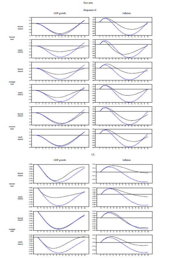
Figure 2C: Counterfactual analysis. Responses of GDP growth and inflation to a monetary policy shock with and without loan demand and supply channels and for specific borrower categories. 20 figures of data plotted as curves, all with x-axis displaying quarters into future from 0 to 15, and y-axis displaying the response ranges.  The 20 panels are divided into two tables.  The first table is a two column, six row table that includes the panels that represent the Euro area banks.  The first column is GDP growth response to loan demand.  The second column is inflation response to loan demand.  The rows represent the kind of loan offered: business demand, business supply, mortgage demand, mortgage supply, consumer demand, and consumer supply, in that order.  The second table shows the plots for the U.S. area banks.  It is a two column, four row table.  The column arrangement is identical to the Euro area table.  The rows represent the kind of loan offered: business loan demand, business loan supply, mortgage loan demand, and mortgage loan supply, in that order.  Each panel has two curves, a response to a monetary policy shock (blue line) and a counterfactual of responses when closing down either the loan supply or loan demand for each type of loans (black line).
First table, first column, first row: Euro area impulse response with business loan demand on GDP growth.  Y-axis ranges from -0.4 to 0.2.  Both responses are convex, visually becoming distinct around periods 3 and 4.  The blue line reaches a minimum value of about -0.36, and the black line reaches a minimum of about -0.3.  The curves cross around period 14 and 15.  At period 15, both curves show responses of about 0.1, with the blue line slightly above the black line.  First table, second column, first row: Euro area impulse response with business loan demand on inflation.  Y-axis ranges from -0.06 to 0.02.  The responses begin as convex, and begin to separate around period 2.  The blue line response reaches a maximum of about 0.015, and the black line response reaches a maximum of about 0.017.  Both curves have an inflection point around period 6.  The blue line response becomes negative between period 3 and 4, and the black line response becomes negative close to period 5.  At period 9 the blue line reaches a minimum of about -0.06, and at period 10 the black line reaches a minimum of about -0.03.  The curves cross between period 14 and 15.  At period 15 the blue line response finishes at just below 0, and the black line response finishes at about -0.01.  First table, first column, second row: Euro area impulse response with business loan supply on GDP growth.  Y-axis ranges from -0.4 to 0.2.  The responses are predominantly convex, visually separating around period 2.  The blue line response reaches a minimum of about -0.36 at periods 7 and 8, and the black line response reaches a minimum of about -0.2 also at period 7 and 8.  First table, second column, second row: Euro area impulse response with business loan supply on inflation.  Y-axis ranges from -0.06 to 0.02.  The responses begin as concave, separating after period 2.  The blue line response reaches a maximum of about 0.015 at period 2, and the black line response reaches a maximum of about 0.01 at period 1.  At around period 5 both responses have an inflection point.  The blue line response becomes negative around period 4, and the black line response becomes negative around period 3.  Between periods 6 and 7 the responses cross.  The black line response reaches a minimum of about -0.045 at period 8, and the blue line response reaches a minimum of about -0.06 at period 9.  The responses cross again between periods 14 and 15.  The blue line response finishes at just below 0, and the black line response finishes at around -0.01.   First table, first column, third row: Euro area impulse response with mortgage loan demand on GDP growth.  Y-axis ranges from -0.4 to 0.2.  The response are predominantly convex, separating around period 2.  The blue line response reaches a minimum of about -0.37 around periods 7 and 8, and the black line response reaches a minimum at about -0.2 also around period 7 and 8.  The responses cross at period 13.  At period 15, the blue line response is about 0.1, and the black line response is about -0.02.  First table, second column, third row: Euro area impulse response with mortgage loan demand on inflation.  Y-axis ranges from -0.06 to 0.03.  The responses begin as concave, separating at around period 1.  The blue line response increases to a maximum of about 0.015 in period 2, and the black line response increases to about 0.02 at period 2.  Around period 6 both responses have an inflection point.  The blue line response becomes negative around period 4, and the black line response becomes negative around period 5.  The blue line response reaches a minimum of about -0.06 at period 9, and the black line response reaches a minimum of about -0.03.  At period 15, both responses are slightly below 0.  First table, first column, fourth row: Euro area impulse response with mortgage loan supply on GDP growth.  Y-axis ranges from -0.4 to 0.2.  Both responses are predominantly convex, with the curves visually separating around period 2.  The blue line response reaches a minimum of about -0.36 around period 7, and the black line response reaches a minimum of about -0.2 around period 6 and 7.  Both responses become positive between period 13 and 14, and cross close to period 14.  At period 15 the blue line response is about 0.1 and the black line response is about 0.05.  Fist table, second column, fourth row: Euro area impulse response with mortgage loan supply on inflation.  Y-axis ranges from -0.06 to 0.02.  The responses begin as concave, with both responses reaching a maximum of about 0.015.  The blue line response becomes negative around period 4, and the black line response becomes negative shortly after the blue response.  An inflection point occurs around period 6 for both curves.  The blue response reaches a minimum of about -0.06 at period 9, and the black line response reaches a minimum of about -0.03 also at period 9.  At period 15, both responses are slightly below 0.  First table, first column, fifth row: Euro area impulse response with consumer loan demand on GDP growth.  Y-axis ranges from -0.4 to 0.2 . Both responses are predominantly convex, and follow each other closely.  Both responses reach a minimum of about -0.35 around period 7 to 8, and both response finish slightly above 0 at period 15.  First table, second column, fifth row: Euro area impulse response with consumer loan demand on inflation.  Y-axis ranges from -0.06 to 0.02.  Both responses began as concave, and both increase to a maximum of about 0.015 at period 2.  The blue line response becomes negative between period 3 and 4, and the black line response becomes negative between periods 4 and 5.  Both responses have an inflection point around period 6.  The black line response reaches a minimum of about -0.04 around period 10, and the blue line response reaches a minimum of about -0.06 around period 0.09.  The responses cross in period 13, and at period 15 the blue line response is slightly below 0, and the black line response is about 0.015.  First table, first column, sixth row: Euro area impulse response with consumer loan supply on GDP growth.  Y-axis ranges from -0.4 to 0.2.  Both responses are predominantly convex, and both responses follow each other very closely.  The responses reach a minimum of about -0.35 around period 8, and both responses becomes positive between period 13 and 14.  At period 15, the responses are around 0.1.  First table, second column, sixth row: Euro area impulse response with consumer loan supply on inflation.  Y-axis ranges from -0.06 to 0.02.  Both responses begin as concave, increasing to about 0.015 at period 2.  The blue line response then becomes negative between period 3 and 4, and the black line response becomes negative close to period 5.  For both responses, an inflection point occurs around period 6.  The blue line response reaches a minimum of about -0.06 at period 9, and the black line response reaches a minimum of about -0.03 around period 11.  The responses cross between periods 13 and 14.  At period 15 the blue line response is slightly below 0, and the black line response is about -0.015.                   
Second table, first column, first row: US impulse response with business loan demand on GDP growth.  Y-axis ranges from -0.2 to 0.  Both responses are predominantly convex, and follow each other closely until period 5.  The black line response reaches a minimum of about -0.175 at period 6, and the blue line response reaches a minimum of about -0.183 at period 7.  At period 15 both responses are near each other, at a level of about -0.05.  Second table, second column, first row: US impulse response with business loan demand on inflation.  Y-axis ranges from -0.03 to 0.02.  Both responses begin as concave, with the blue response reaching a maximum of about 0.01 at period 3, and the black response reaching a maximum of about 0.016 at period 4.  The blue response becomes negative around period 6, and has an inflection point at period 9.  The black response becomes negative around period 12, with an inflection point at period 10.  At period 15 the blue response reaches a minimum of about -0.027, and the black response reaches a minimum of just under 0.  Second table, first column, second row: US impulse response with business loan supply on GDP growth.  Y-axis ranges from -0.2 to 0.  Both responses are predominantly convex, with the blue line response reaching a minimum of about -0.183, and the black line response reaching a minimum of about -0.1.  Around period 15 the responses cross at a level of about -0.05.  Second table, second column, second row: US impulse response with business loan supply on inflation.  Y-axis ranges from -0.03 to 0.015.  Both responses begin as concave, with the blue response and black response reaching a maximum of about 0.01 at period 3.  The blue response becomes negative around period 6, and has an inflection point at period 9.  The black response becomes negative around period 10, with an inflection point at period 10.  At period 15 the blue response reaches a minimum of about -0.025, and the black response reaches a minimum of just under -0.005.  Second table, first column, third row: US impulse response with mortgage loan demand on GDP growth.  Y-axis ranges from -0.2 to 0.  The responses are almost completely convex, and follow each other very closely.  Both responses reach a minimum of about -0.183 around period 7, and both responses end at about -0.05 at period 15.  Second table, second column, third row: US impulse response with mortgage loan demand on inflation.  Y-axis ranges from -0.03 to 0.015.  The responses begin as concave, and follow each other very closely throughout the response.  Both curves become negative between period 6 and 7, and have an inflection point at around period 8.  At period 15, the responses reach a minimum of about -0.025.  Second table, first column, fourth row: US impulse response with mortgage loan supply on GDP growth.  Y-axis ranges from -0.2 to 0.025.  The responses are predominantly convex, with the blue line response decreasing to a minimum of about -0.0183, and the black line response falling to a minimum of about -0.125.  At period 15 the blue line response is about -0.05, and the black line response ends at just above 0.  Second table, second column, fourth row: US impulse response with mortgage loan supply and inflation.  Y-axis ranges from -0.03 to 0.02.  The responses begin as concave, with the blue line response increasing to a maximum of about 0.01 at period 3, and the black line response increasing to a maximum of about 0.015 at period 4.  The blue line response becomes negative between period 6 and 7, and the black response becomes negative between periods 8 and 9.  At period 10 both responses have an inflection point.  At period 15, the blue line response is about -0.025, and the black line response is about -0.01.
Note: These graphs report counterfactual experiments. The responses of output growth and inflation to a one-standard deviation monetary policy shock are compared with the responses obtained when closing down the credit channels (demand or supply). All types of loans are considered. Responses of the series are normalised and divided by their innovation variances so that all responses to a shock are comparable on a single scale. The graphs on the first six rows refer to the Euro area. The last four rows shows the responses for the United States (US). The panel VAR for the Euro Area is estimated assuming fixed effects, slope homogeneity and the country identification strategy as explained in Section 3. The specification of the VAR includes 9 variables: GDP growth, inflation, overnight rates, demand and supply (two channels) for each type of loans (see MODEL 2 in Section 3.5). See Section 3 and Appendix for a detailed definition of the variables.

Figure 2D: Couterfactual analysis. Responses of GDP growth and inflation to a loan supply shock with and without loan demand channels (for a specific borrower category)
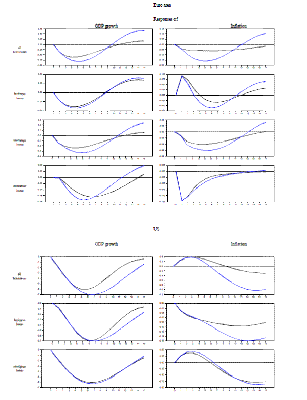
Figure 2D: Counterfactual analysis.  Responses of GDP growth and inflation to a loan supply shock with and without loan demand and supply channels (for specific borrower categories).  14 figures of data plotted as curves, all with x-axis displaying quarters into future from 0 to 15, and y-axis displaying the response ranges.  The 14 panels are divided into two tables.  The first table is a two column, four row table that includes the panels that represent the Euro area banks.  The first column is GDP growth response to loan demand.  The second column is inflation response to loan demand.  The rows represent the kind of loan offered: all borrowers, business loans, mortgage loans, and consumer loans, in that order.  The second table shows the plots for the U.S. area banks.  It is a two column, three row table.  The column arrangement is identical to the Euro area table.  The rows represent the kind of loan offered: all borrowers, business loans, and mortgage loans, in that order.  Each panel has two curves, a response to a monetary policy shock (blue line) and a counterfactual of responses when closing down either the loan supply or loan demand for each type of loans (black line).
First table, first column, first row: Euro area impulse response with all borrowers on GDP growth.  Y-axis ranges from -1 to 0.75.  Both responses begin as convex, with the black line response reaching a minimum of about -0.6 at period 3, and the blue line response reaching a minimum of about -0.75 at period 4.  Both responses have an inflection point around period 8.  The responses cross at period 9, at a level of about -0.25.  The blue line becomes positive between period 9 and 10, and the black line becomes positive between around period 11.  At period 15 the blue line response ends at about 0.75 and the black line response ends at about 0.25.  First table, second column, first row: Euro area impulse response with all borrowers on inflation.  Y-axis ranges from -0.2 to 0.15.  Both responses rise are predominantly convex, with the blue line response reaching a minimum of about -0.15 at period 5, and the black line response reaching a minimum of about -0.05 around period 6.  The responses cross between periods 9 and 10 at a level of about -0.05.  The blue line becomes positive at period 11.  At period 15, the blue line response is about 0.1, and the black line response is slightly below 0.  First table, first column, second row: Euro area impulse response with business loans on GDP growth.  Y-axis ranges from -0.5 to 0.5.  Both responses begin as convex, with the black line response reaching a minimum of about -0.38 at period 3, and the blue line response reaching a minimum of about -0.4 at period 4.  Both responses have an inflection point between periods 8 and 9.  Both responses become positive close to period 9.  The responses cross between periods 9 and 10, at a level of about 0.14.  At period 15 the blue line response ends at about 0.4 and the black line response ends at about 0.35.  First table, second column, second row: Euro area impulse response with business loans on inflation.  Y-axis ranges from -0.075 to 0.1.  Both responses rise to a maximum of about 0.09 at period 1, after which the curves are predominantly convex, with the blue line response reaching a minimum of about -0.05 at period 6, and the black line response reaching a minimum of about -0.025 around period 7.  The responses cross between periods 9 and 10 at a level of about -0.02.  The blue line becomes positive at period 10, and the black line response becomes positive at period 11.  At period 15, the blue line response is about 0.075, and the black line response is about 0.025.  First table, first column, third row: Euro area impulse response with mortgage loans on GDP growth.  Y-axis ranges from -0.4 to 0.3.  Both responses begin as convex, with the black line response reaching a minimum of about -0.2 at period 4, and the blue line response reaching a minimum of about -0.3 at period 5.  Both responses have an inflection point around period 9.  The responses cross shortly after period 10, at a level of about -0.1.  The blue line becomes positive between period 10 and 11, and the black line becomes positive between period 11 and 12.  At period 15 the blue line response ends at about 0.2 and the black line response ends at about 0.06.  First table, second column, third row: Euro area impulse response with mortgage loans on inflation.  Y-axis ranges from -0.08 to 0.04.  Both responses are predominantly convex, with the black line response reaching a minimum of about -0.04 at period 5, and the blue line response reaching a minimum of about -0.06 around period 6.  The responses cross between periods 10 and 11 at a level of about -0.02.  The blue line becomes positive at period 12, and the black line response becomes positive at period 15.  At period 15, the blue line response is about 0.03, and the black line response is just above 0.  First table, first column, fourth row: Euro area impulse response with consumer loans on GDP growth.  Y-axis ranges from -0.08 to 0.04.  Both responses begin as convex, with the blue line response reaching a minimum of about -0.07 at period 5, and the black line response reaching a minimum of about -0.06 at period 7.  The responses cross at period 7, at a level of about -0.06.  The blue line response has an inflection point around period 11, where an inflection point also occurs.  The blue line becomes positive between period 11 and 12, and the black line becomes positive between around period 14.  At period 15 the blue line response ends at about 0.04 and the black line response ends at about 0.01.  First table, second column, fourth row: Euro area impulse response with consumer loans on inflation.  Y-axis ranges from -0.125 to 0.025.  Both responses begin as convex, with both responses reaching a minimum of about -0.125 at period 1.  At period 3 the responses experience an inflection point.  The responses cross between periods 10 and 11 at a level of about -0.01.  The blue line becomes positive at period 13.  At period 15, the blue line response is just above 0, and the black line response is slightly below 0.    
Second table, first column, first row: US impulse response with all borrows on GDP growth.  Y-axis ranges from -7 to 0.  Both responses are predominantly convex, with the black response reaching a minimum of about -6 at period 6, and the blue response reaching a minimum of about -7 at period 7.  At period 15 the black response is about -0.5, and the blue response is about -2.  Second table, second column, first row: US impulse response with all borrowers on inflation.  Y-axis ranges from -1.2 to 0.4.  Both responses start as concave, with both reaching a maximum of about 0.4 at period 3.  The blue line response becomes negative at period 6, and the black line response becomes negative at period 9.  Both responses have an inflection point around period 9.  At period 15 the blue line response is about -1, and the black line response is about -0.4.  Second table, first column, second row: US impulse response with business loans on GDP growth.  Y-axis ranges from -0.7 to 0.  Both responses are predominantly convex, and follow each other closely until period 8.  The responses reach a minimum of about -0.7 around period 7.  At period 15 the black response is about -0.1, and the blue response is about -0.2.  Second table, second column, second row: US impulse response with business loans on inflation.  Y-axis ranges from -0.16 to 0.  Both responses are predominantly convex.  The black line response reaches a minimum of about -0.1 around period 10.  The blue line response reaches a minimum of about -0.16 around period 12.  At period 15, the black line response is about -0.08, and the blue line response is about -0.14.  Second table, first column, second row: US impulse response with business loans on GDP growth.  Y-axis ranges from -0.7 to 0.  Both responses are predominantly convex, and follow each other closely throughout the response.  The responses reach a minimum of about -6 around period 7.  At period 15 the responses are about -2.  Second table, second column, third row: US impulse response with mortgage loans on inflation.  Y-axis ranges from -1 to 0.5.  Both responses start as concave and follow each other closely, with both reaching a maximum of about 0.4 at period 3.  The responses become negative between period 6 and 7.  Both responses have an inflection point around period 8.  At period the responses are about -0.75.
Note: These graphs report counterfactual experiments. The responses of output growth and inflation to a credit supply shock are compared with the responses obtained when closing down the demand channel. All types of loans are considered. Responses of the series are normalised and divided by their innovation variances so that all responses to a shock are comparable on a single scale. The graphs on the first six rows refer to the Euro area. The last four rows shows the responses for the United States (US). The panel VAR for the Euro Area is estimated assuming fixed effects, slope homogeneity and the country identification strategy as explained in Section 3. The specification of the VAR includes 9 variables: GDP growth, inflation, overnight rates, demand and supply (two channels) for each type of loans (see MODEL 2 in Section 3.5). See Section 3 and Appendix for a detailed definition of the variables.

Figure 3A: Firm balance-sheet and bank lending channel. Responses of demand and supply of business loans to a monetary policy shock
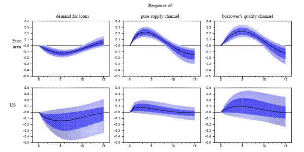
Figure 3A: Firm Balance-Sheet and bank lending channel. Responses of demand and supply of business loans to a monetary policy shock.
This figure has six panels showing the Euro area's and the US's response of demand for loans, pure supply channel and borrower's quality channel to a one-standard deviation monetary policy shock. The 68% Bayesian credible interval is dark blue, and the 90% Bayesian credible interval is light blue.  The y-axes go from -0.5 to 0.4 and the x-axes go from 0 to 15. 
In the first panel, which is the Euro area's response of demand for loans, the line starts at (0,0) before dipping into a shallow u-shape with a low-point of a little below -0.1 at 5. It crosses the y-value of 0 at 12 and the line ends at about 0.05 at 15.
In the second panel, which is the Euro area's response of pure loan supply, the line starts at (0,0) and sharply increases to a peak of 0.2 at 3.  It decreases and crosses the y-value of 0 at 9 and ends at -0.15 at 15.
In the third panel, which is the Euro area's response of borrower's quality loans, the line starts at (0,0) and increases to 0.2 at 5 before decreasing. It crosses the y-value of 0 at 11 and ends o the down-slope at -0.1 at 15.
In the fourth panel, which is the US's response of demand for loans, the line starts at (0,0) and slopes down reaching a trough of -0.1 before gradually sloping upwards again, stopping just below the y-value of 0 at 15.
In the fifth panel, which is the US's response of pure loan supply, the line starts at (0,0) and increases to a peak of 0.1 and then gradually slopes down and stop just below 0 at 15.
In the sixth panel, which is the US's response of borrower's quality loans, the line starts at (0,0) and increases to a peak of 0.1 at 4 and then gradually decrease and reaches slightly below 0 at 15.
Note: These graphs plot the responses of loan demand and loan supply to a one-standard deviation monetary policy shock. Only business loans (loans to non-financial corporations) are considered. Loan supply is represented by two different channels: the pure supply and the borrower's quality channel (proxy for the bank lending and the firm balance-sheet channel). Responses of the series are normalised and divided by their innovation variances so that all responses to a shock are comparable on a single scale. The median response is shown along with 68 (dark blue) and 90 (light blue) percent Bayesian credible intervals, computed by estimating the VAR with a flat prior on the parameters and assuming normality of the error terms. The graphs on the first row refer to the Euro area, while the second row shows the responses for the United States (US). The panel VAR for the Euro Area is estimated assuming fixed effects, slope homogeneity and the country identification strategy as explained in Section 3. The specification of the VAR includes 6 variables for the euro area: GDP growth, inflation, demand and supply (two variables) for business loans (see MODEL 3 in Section 3.5.). See Section 3 and Appendix for a detailed definition of the variables.

Figure 3B: Firm balance-sheet and bank lending channel. Responses of GDP growth and inflation to a shock to loan demand and loan supply
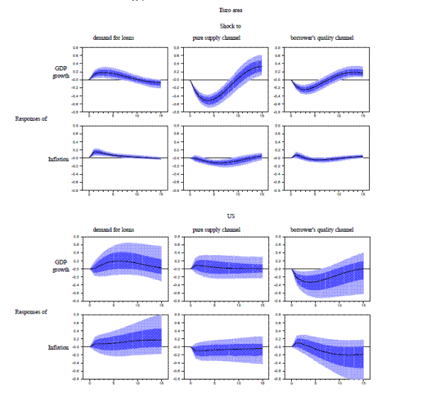
Figure 3B: Firm balance-sheet and bank lending channel. Responses of GDP growth and inflation to a shock to loan demand and loan supply.
This figure has twelve panels that graph the US and the Euro area's response of GDP growth and inflation to shocks to demand for loans, to the pure supply channel and to the borrower's quality channel. The 68% Bayesian credible interval is dark blue, and the 90% Bayesian credible interval is light blue.  The y-axes go from -0.8 to 0.8 and the x-axes go from 0 to 15.  It should be noted that the credible intervals for the US are much larger than those for the Euro area.
In the first panel, which is the Euro area's response of GDP growth to a shock to demand for loans, the line starts at (0,0) before increasing to a peak of 0.2 at 3 and then decreasing gradually. It crosses the y-value of 0 at 9 and ends at -0.1 at 15.
In the second panel, which is the Euro area's response of GDP growth to a shock to the pure supply channel, the line starts at (0,0) before sharply decreasing to a trough of -.5 at 4. It then increases steadily, crossing the y-axis at 10 and ending at 0.3 at 15.
In the third panel, which is the Euro area's response of GDP growth to a shock in the borrower's quality channel, the line starts at (0,0) before sloping down briefly, reaching a low-point of -0.2 at 3 and then crossing the y-axis at 8 before briefly reaching a point at 0.2 and ending just slightly below 0.2 at 15.
In the fourth panel, which is the Euro area's response of inflation to a shock to demand for loans, the line starts at (0,0) before increasing to 0.2 at 1, then very steadily declining again, reaching the y-axis just before 15.
In the fifth panel, which is the Euro area's response of inflation to a shock to the pure supply channel, the line starts and (0,0) before slowly decreasing to a trough of -0.1 at 6. It then slowly increases, crossing the y-axis at 12 and then ending at 0.1 at 15.
In the sixth panel, which is the Euro area's response of inflation to a shock to the borrower's quality channel, the line start at (0,0) before increasing slightly to 0.1 at 1, and then swooping down, reaching a low-point just below the y-axis  at 6 and then very, very gradually increasing again to end at just above 0 at 15.
In the seventh panel, which is the US's response of GDP growth to a shock to demand for loans, the line starts at (0,0) before increasing to a peak of 0.2 at 6 and then decreasing gradually, then ending just slightly above the y-axis at 15.
In the eighth panel, which is the US's response of GDP growth to a shock to the pure supply channel, the line starts at (0,0) before increasing to a peak of 0.1 at 1. It then decreases slightly until 5, where it really starts to flatten out, and then ends at the y-axis at 15.
In the ninth panel, which is the US's response of GDP growth to a shock in the borrower's quality channel, the line starts at (0,0) before decreasing to a trough of -0.3 at 4. It then increases with a decreasing rate until it ends at the y-axis right at 15.
In the tenth panel, which is the US's response of inflation to a shock to demand for loans, the line starts at (0,0) before increasing to 0.1 at 1. It then continues to increase at a slower rate, finally flattening out and ending at 0.2 at 15.
In the eleventh panel, which is the US's response of inflation to a shock to the pure supply channel, the line starts and (0,0) before sharply decreasing to a trough of -0.1 at 1. It then slowly increases,  just below the y-axis at 15.
In the twelfth panel, which is the US's response of inflation to a shock to the borrower's quality channel, the line start at (0,0) before quickly increasing to 0.1 at 1, and then swooping down where it reaches a low-point and generally flattens out at -0.2 at 11. It just barely increases again after that until it ends at 15.
Note: These graphs plot the reesponses of GDP growh and inflation to a one-standard deviation shock of loan demand and loan supply. Only business loans (loans to non-financial corporations) are considered. Loan supply is represented by two different channels: the pure supply and the borrower's quality channel (proxy for the bank lending and the firm balance-sheet channel). Responses of the series are normalised and divided by their innovation variances so that all responses to a shock are comparable on a single scale. The median responses is shown along with 68 (dark blue) and 90 (light blue) percent Bayesian credible intervals, computed by estimating the VAR with a flat prior on the parameters and assuming normality of the error terms. The graphs on the first two rows refer to the Euro area (EA), while the other rows show the responses for the United States (US). The panel VAR for the Euro Area is estimated assuming fixed effects, slope homogeneity and the country identification strategy as explained in Section 3. The specifcation of the VAR includes 6 variables for the euro area: GDP growth, inflation, demand and supply (two variables) for business loans (see MODEL 3 in Section 3.5.). See Section 3 and Appendix for a detailed definition of the variables.

Figure 3C. Counterfactual analysis. Firm balance-sheet and bank lending channel. Responses of GDP growth and inflation to a monetary policy shock.
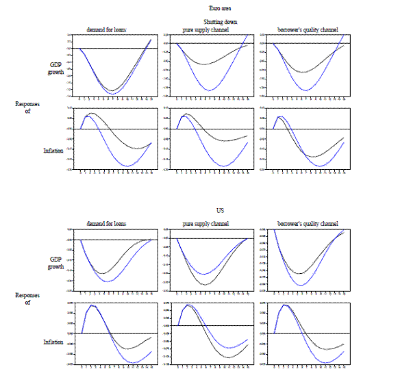
Figure 3C: Counterfactual Analysis. Firm balance-sheet and bank lending channel. Responses of GDP growth and inflation to a monetary policy shock.
This figure has 12 panels that compare the response of GDP growth and inflation to a one-standard deviation monetary policy shock  with a shutting down in the demand for loans, in the pure supply channel and in the borrower's quality channel and for both the US and the Euro area.  The blue line is the response to the monetary policy shock (and thus is the same across the three graphs for GDP growth and the three graphs for inflation for each country), and the black line is the response to the shutting down in the demand or supply of loans.
In the first panel, which is the Euro area's response of GDP growth to the shutting down in the demand for loans, the blue starts at (0,0) and dips down to -0.13 at 7 before increasing, crossing the y-axis at 14 and ending at 0.2 at 15.  The black line stays with the blue line for the most part, though it reaches a low-point slightly above, just as -0.12 and crosses the y-axis just slightly before the blue line does.  Both liens end in virtually the same place.
In the second panel, which is the Euro area's GDP growth response to a shutting down in the pure supply channel, the blue line starts at (0,0) and dips down to -0.13 at 7 before increasing, crossing the y-axis at 14 and ending at 0.2 at 15. The black line stays with the blue line until it reaches almost -0.25 at 1. Its rate of decrease then slows and it bottoms-out in a much shallower trough than the blue line, reaching a low-point of -0.50 at 6. It then increases and crosses the blue line at  -0.12 at 14 before ending just below the y-axis at 15.
In the third panel, which is the Euro area's GDP growth response to a shutting down in the borrower's quality channel, the blue line starts at (0,0) and dips down to -0.13 at 7 before increasing, crossing the y-axis at 14 and ending at 0.2 at 15. The black line follows an almost identical pattern as in the second panel, except it troughs slightly lower at -0.80.
In the fourth panel, which is the Euro area's inflation response to shutting down in the demand for loans, the blue lines starts at (0,0) and rapidly increases to a peak of 0.06 at 2 before decreasing, crossing the y-axis at 4 and reaching a trough of -0.18 at 10 and increasing again to end at -0.07 at 15.  The black line mimics the shape, though it reaches a higher peak of 0.08 at 3, crosses the y-axis at 6 and troughs at -0.09 at 12, before ending aT virtually the same point as the blue line.
In the fifth panel, which is the Euro area's inflation response to a shutting down in the pure supply channel, the blue lines starts at (0,0) and rapidly increases to a peak of 0.06 at 2 before decreasing, crossing the y-axis at 4 and reaching a trough of -0.18 at 10 and increasing again to end at -0.07 at 15.  The black line mimics the shape of the blue line, though it peaks at 0.08 at 2.5, crosses the y-axis at 6, troughs at -0.06 at 10 and ends at -0.04 at 15, above the end point for the blue line.
In the sixth panel, which is the Euro area's inflation response to a shutting down in the borrower's demand channel, the blue lines starts at (0,0) and rapidly increases to a peak of 0.06 at 2 before decreasing, crossing the y-axis at 4 and reaching a trough of -0.18 at 10 and increasing again to end at -0.07 at 15.  The black line has a similar shape, though it peaks only at 0.05 at 1, crosses the y-axis early at 3, and has a shallower trough so that it crosses the blue line at -0.12 at 7 and reaches a trough of -0.14 at 9. It ends at -0.05 above the blue line.
In the seventh panel, which is the US's response of GDP growth to the shutting down in the demand for loans, the blue line starts at (0,0) and dips down to -0.20 at 6 before increasing and ending at the y-axis at 15.  The black line stays with the blue line until -0.12 at 2 before reaching a shallower trough at -0.11 and increasing, crosses the y-axis at 14 and ending just slightly above 0 at 15.
In the eight panel, which is the US's GDP growth response to a shutting down in the pure supply channel, the blue line starts at (0,0) and dips down to -0.20 at 6 before increasing and ending at the y-axis at 15. The black line stays with the blue line until it reaches almost -0.08 at 1. Its rate of decrease is faster than that of the blue line and so it reaches a trough below that of the blue line, reaching a low-point of -0.27 at 6. It then increases and meets the blue line again just before it ends at the y-axis at 15.
In the ninth panel, which is the US's GDP growth response to a shutting down in the borrower's quality channel, the blue line starts at (0,0) and dips down to -0.13 at 7 before increasing, crossing the y-axis at 14 and ending at 0.2 at 15. The black line follows a similar trajectory to the blue line, except that it troughs higher at -0.160 and stays above the blue line, until they cross at -0.025 at 14. The black line ends at about -0.010 at 15.
In the tenth panel, which is the US's inflation response to shutting down in the demand for loans, the blue lines starts at (0,0) and rapidly increases to a peak of 0.07 at 2 before decreasing, crossing the y-axis at 6 and reaching a trough of -0.073 at 11 and increasing again to end at -0.045 at 15.  The black line mimics the shape, only separating from the blue line just before they hit the y-axis. The black line then dips into a shallower trough, with its low-point at -0.035 and it ends at -0.010 at 15. 
In the eleventh panel, which is the US's inflation response to a shutting down in the pure supply channel, the blue lines starts at (0,0) and rapidly increases to a peak of 0.07 at 2 before decreasing, crossing the y-axis at 6 and reaching a trough of -0.073 at 11 and increasing again to end at -0.045 at 15.  The black line mimics the shape of the blue line, but after the peak it decreases more quickly, crossing the y-axis at 5 and then reaching its trough at -0.100 at 11 and rising again, ending at -0.06 at 15.
In the twelfth panel, which is the US's inflation response to a shutting down in the borrower's demand channel, the blue lines starts at (0,0) and rapidly increases to a peak of 0.07 at 2 before decreasing, crossing the y-axis at 6 and reaching a trough of -0.073 at 11 and increasing again to end at -0.045 at 15.  The black line has a similar shape, though after the peak it decreases at a slower rate than the blue line and crosses the y-axis at 7. It reaches a higher low-point at -0.030 at 11 and ends at -0.025 at 15.
Note: These graphs report counterfactual experiments. The responses of output growth and inflation to a one-standard deviation monetary policy shock are compared with the responses obtained when closing down the credit channels (one demand channel and two supply channels). Only business loans are considered. Responses of the series are normalised and divided by their innovation variances so that all responses to a shock are comparable on a single scale. The graphs on the first two rows refer to the Euro area. The last two rows show the responses for the United States (US). The panel VAR for the Euro Area is estimated assuming fixed effects, slope homogeneity and the country identificatio strategy as explained in Section 3. The specification of the VAR includes 6 variables: GDP growth, inflation, overnight rates, demand and supply (two channels) for business loans (see MODEL 3 in Section 3.5). See Section 3 and Appendix for a detailed definition of the variables.

Figure 4A: Responses of loan demand and supply (bank lending and borrower's bank lending channels) to a monetary policy shock (all category of borrowers).
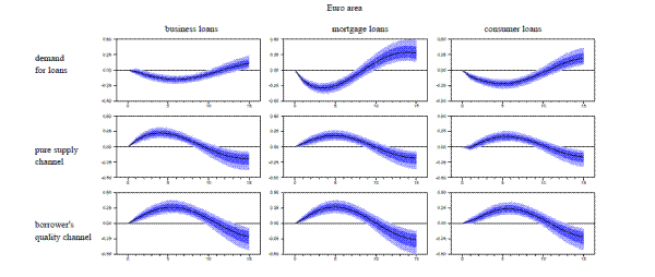
Figure 4A: Responses of loan demand and supply (bank lending and borrower's bank lending channels) to a monetary policy shock (all category of borrowers). Responses of loan demand and supply (bank lending and borrower's bank lending channels) to a monetary policy shock (all category of borrowers); Euro area.  9 figures of data plotted as curves, all with x-axis displaying quarters into future from 0 to 15, and y-axis displaying the response, with a range from -0.5 to 0.5.  The figures are arranged into a three column, three row matrix.  The columns separate the type of loan: business loans, mortgage loans, and consumer loans, in that order.  The rows represent the monetary tightening channel: demand for loans, pure supply channel, and borrower's quality channel, in that order.  Each panel has a black median response curve, along with 68 and 90 percent Bayesian credible intervals.  
First column, first row: response with demand for loans and business loans.  The response begins as convex, decreasing a minimum of about -0.15 around period 6.  Around period 9 an inflection point occurs, and the response becomes positive around period 12.  At period 15 the response is about 0.1.  Bayesian intervals: at period 5 the 68 percent interval is about 0.08 and the 90 percent interval is about 0.1.  At period 15 the 68 percent interval is about 0.1 and the 90 percent interval is about 0.2.  Second column, first row: response with demand for loans and mortgage loans.  The response begins as convex, decreasing a minimum of about -0.25 around period 3.  Around period 8 an inflection point occurs, and the response becomes positive between period 8 and 9.  At period 15 the response is about 0.25.  Bayesian intervals: at period 5 the 68 percent interval is about 0.08 and the 90 percent interval is about 0.1.  At period 15 the 68 percent interval is about 0.2 and the 90 percent interval is about 0.3.  Third column, first row: response with demand for loans and consumer loans.  The response begins as convex, decreasing a minimum of about -0.2 around period 5.  Around period 10 an inflection point occurs, and the response becomes positive around period 11.  At period 15 the response is about 0.2.  Bayesian intervals: at period 5 the 68 percent interval is about 0.08 and the 90 percent interval is about 0.1.  At period 15 the 68 percent interval is about 0.15 and the 90 percent interval is about 0.25.  First column, second row: response with the pure supply channel and business loans.  The response begins as concave, increasing to a maximum of about 0.25 at period 4.  At period 9 the response becomes negative, as well as experiencing an inflection point.  At period 15 the response is about -0.2.  Bayesian intervals: at period 5 and the 68 percent interval is about 0.08 and the 90 percent interval is about 0.1.  At period 15 the 68 percent interval is about 0.15, and the 90 percent interval is about 0.25.  Second column, second row: response with the pure supply channel and mortgage loans.  The response begins as concave, increasing to a maximum of about 0.22 at period 5.  At period 10 the response becomes negative, as well as experiencing an inflection point.  At period 15 the response is about -0.2.  Bayesian intervals: at period 5 and the 68 percent interval is about 0.08 and the 90 percent interval is about 0.1.  At period 15 the 68 percent interval is about 0.15, and the 90 percent interval is about 0.25.  Third column, second row: response with the pure supply channel and consumer loans.  The response begins as concave, increasing to a maximum of about 0.2 at period 5.  Between period 10 and 11 the response becomes negative, as well as experiencing an inflection point.  At period 15 the response is about -0.18.  Bayesian intervals: at period 5 and the 68 percent interval is about 0.08 and the 90 percent interval is about 0.1.  At period 15 the 68 percent interval is about 0.15, and the 90 percent interval is about 0.25.  First column, third row: response with the pure supply channel and business loans.  The response begins as concave, increasing to a maximum of about 0.25 at period 6.  At period 11 the response becomes negative, as well as experiencing an inflection point.  At period 15 the response is about -0.25.  Bayesian intervals: at period 5 and the 68 percent interval is about 0.1 and the 90 percent interval is about 0.14.  At period 15 the 68 percent interval is about 0.2, and the 90 percent interval is about 0.3.  Second column, third row: response with the pure supply channel and business loans.  The response begins as concave, increasing to a maximum of about 0.25 at period 5.  At period 11 the response becomes negative, as well as experiencing an inflection point.  At period 15 the response is about -0.25.  Bayesian intervals: at period 5 and the 68 percent interval is about 0.1 and the 90 percent interval is about 0.14.  At period 15 the 68 percent interval is about 0.2, and the 90 percent interval is about 0.35.  Third column, third row: response with the pure supply channel and business loans.  The response begins as concave, increasing to a maximum of about 0.25 at period 6.  At period 11 the response becomes negative, as well as experiencing an inflection point.  At period 15 the response is about -0.25.  Bayesian intervals: at period 5 and the 68 percent interval is about 0.1 and the 90 percent interval is about 0.14.  At period 15 the 68 percent interval is about 0.18, and the 90 percent interval is about 0.3.
Note: These graphs report the responses of loan demand and loan supply (via bank lending and borrower's balance sheet channels) to a monetary policy shock for all borrower's category. Responses of the series are normalised and divided by their innovation variances so that all responses to a shock are comparable on a single scale. The median response is shown along with 68 (dark blue) and 90 (light blue) percent Bayesian credible interals, computed y estimating the VAR with a flat prior on the parameters and assuming normality of the error terms. The graphs refer to the Euro area. The panel VAR for the Euro Area is estimated assuming fixed effects, slope homogeneity and the country identification strategy as explained in Section 3. The specification of the VAR includes 9 variables: GDP growth, inflation, overnight rates, demand and supply (two channels) for all type of loans (see MODEL 4 in Section 3.5.) See Section 3 and Appendix for a detailed definition of the variables.

Figure 4B: Responses of Euro area GDP growth and inflation to a shock to loan demand and loan supply (bank lending and borrower's balance sheet channel), all category of borrowers.
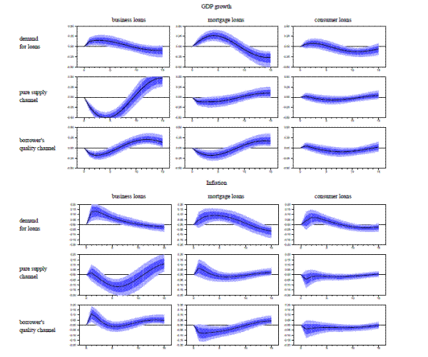
Figure 4B: Responses of Euro area GDP growth and inflation to a shock to loan demand and loan supply (bank lending and borrower's balance sheet channel), all category of borrowers.  18 figures of data plotted as curves, all with x-axis displaying quarters into future from 0 to 15, and y-axis displaying the response.  The figures are arranged into two table of 9, one for GDP growth response, the other for inflation response.  All figures in the GDP table have y-axis range of -0.5 to 0.5, and all figures in the inflation table have y-axis range of -0.2 to 0.2.  Each table arrangement has three columns and three rows.  The columns separate the type of loan: business loans, mortgage loans, and consumer loans, in that order.  The rows represent the monetary tightening channel: demand for loans, pure supply channel, and borrower's quality channel, in that order.  Each panel has a black median response curve, along with 68 and 90 percent Bayesian credible intervals.  
First table, first column, first row: response with business loan demand on GDP growth.  The response begins as concave, increasing to a maximum of about 0.15 at period 2.  At period 9 the response becomes negative, as well as experiencing an inflection point.  At period 15 the response is about -0.1.  Bayesian intervals: at period 5 and the 68 percent interval is about 0.15 and the 90 percent interval is about 0.25.  At period 15 the 68 percent interval is about 0.15, and the 90 percent interval is about 0.25.  First table, second column, first row: response with mortgage loan demand on GDP growth.  The response begins as concave, increasing to a maximum of about 0.25 at period 4.  At period 9 the response becomes negative, as well as experiencing an inflection point.  At period 15 the response is about -0.25.  Bayesian intervals: at period 5 and the 68 percent interval is about 0.15 and the 90 percent interval is about 0.25.  At period 15 the 68 percent interval is about 0.2, and the 90 percent interval is about 0.35.  First table, third column, first row: response with consumer loan demand on GDP growth.  The response begins as concave, increasing to a maximum of about 0.08 at period 2.  At period 6 the response becomes negative, as well as experiencing an inflection point.  Around period 11, the response has a minimum of about -0.15.  At period 15 the response is about -0.1.  Bayesian intervals: at period 5 and the 68 percent interval is about 0.15 and the 90 percent interval is about 0.2.  At period 15 the 68 percent interval is about 0.15, and the 90 percent interval is about 0.25.  First table, first column, second row: responses with business loan pure supply channel on GDP growth.  The response begins as convex, decreasing to a minimum of about -0.5 at period 4.  Between period 9 and 10 the function becomes positive, when the response also has an inflection point.  At period 15 the response reaches a maximum of about 0.5.  Bayesian intervals: at period 5 the 68 percent interval is about 0.15, and the 90 percent interval is about 0.25.  At period 15 the 68 percent interval is about 0.2 and the 90 percent interval is about 0.3.  First table, second column, second row: responses with mortgage loan pure supply channel on GDP growth.  The response begins as convex, decreasing to a minimum of about -0.15 at period 2.  At period 9 the function becomes positive, when the response also has an inflection point.  At period 15 the response reaches a maximum of about 0.1.  Bayesian intervals: at period 5 the 68 percent interval is about 0.15, and the 90 percent interval is about 0.25.  At period 15 the 68 percent interval is about 0.2 and the 90 percent interval is about 0.25.  First table, third column, second row: responses with consumer loan pure supply channel on GDP growth.  The response stays close to zero throughout the response range.  Bayesian intervals: for all period, the 68 percent interval is about 0.1 and the 90 percent interval is about 0.2.  First table, first column, third row: responses with business loan borrower's quality channel on GDP growth.  The response begins as convex, decreasing to a minimum of about -0.2 at period 2.  At period 7 the function becomes positive, when the response also has an inflection point.  At period 12 the response reaches a maximum of about 0.2.  At period 15 the response is about 0.1.  Bayesian intervals: at period 5 the 68 percent interval is about 0.15, and the 90 percent interval is about 0.25.  At period 15 the 68 percent interval is about 0.2 and the 90 percent interval is about 0.5.  First table, second column, third row: responses with mortgage loan borrower's quality channel on GDP growth.  The response begins as convex, decreasing to a minimum of about -0.2 at period 2.  At period 7 the function becomes positive, when the response also has an inflection point.  At period 15 the response reaches a maximum of about 0.15.  Bayesian intervals: at period 5 the 68 percent interval is about 0.15, and the 90 percent interval is about 0.25.  At period 15 the 68 percent interval is about 0.2 and the 90 percent interval is about 0.5.  First table, third column, third row: responses with consumer loan borrower's quality channel on GDP growth.  The response stays close to zero throughout the response range.  Bayesian intervals: for all period, the 68 percent interval is about 0.1 and the 90 percent interval is about 0.2.  
Second table, first column, first row: response with business loan demand on inflation.  The response begins as concave, increasing to a maximum of about 0.12 at period 3.  Around period 4 the response has an inflection point, with the response becoming negative around period 10.  At period 15 the response is slightly below 0.  Bayesian intervals:  at period 5 the 68 percent interval is about 0.06, and the 90 percent interval is about 0.08.  At period 15 the 68 percent interval is about 0.04, and the 90 percent interval is about 0.06.  Second table, second column, first row: response with mortgage loan demand on inflation.  The response begins as concave, increasing to a maximum of about 0.08 at period 4.  Around period 11 the response becomes negative and experiences an inflection point.  At period 15 the response is about -0.05.  Bayesian intervals:  at period 5 the 68 percent interval is about 0.06, and the 90 percent interval is about 0.1.  At period 15 the 68 percent interval is about 0.05, and the 90 percent interval is about 0.1.  Second table, third column, first row: response with consumer loan demand on inflation.  The response begins as concave, increasing to a maximum of about 0.07 at period 2.  Around period 6 the response has an inflection point, with the response becoming negative around period 8.  At period 15 the response is slightly below 0.  Bayesian intervals:  at period 5 the 68 percent interval is about 0.05, and the 90 percent interval is about 0.1.  At period 15 the 68 percent interval is about 0.04, and the 90 percent interval is about 0.06.  Second table, first column, second row: response with business loan pure supply channel on inflation.  After a brief increase to slightly above 0 at period 1, the response is predominantly convex, decreasing to a minimum of about -0.12 at period 6.  At period 11 the response becomes positive.  At period 15 the response is about 0.1.  Bayesian intervals: at period 5 the 68 percent interval is about 0.08, and the 90 percent interval is about 0.15.  At period 15 the 68 percent interval is about 0.1, and the 90 percent interval is about 0.15.  Second table, second column, second row: response with mortgage loan pure supply channel on inflation.  After a brief increase to about 0.05, the response stays close to 0 throughout the rest of the time period.  Bayesian intervals: at period 5 the 68 percent interval is about 0.05, and the 90 percent interval is about 0.1.  At period 15 the 68 percent interval is about 0.03, and the 90 percent interval is about 0.05.  Second table, third column, second row: response with consumer loan pure supply channel on inflation.  After a brief decrease to about -0.05, the response stays close to 0 throughout the rest of the time period.  Bayesian intervals: at period 5 the 68 percent interval is about 0.03, and the 90 percent interval is about 0.06.  At period 15 the 68 percent interval is about 0.02, and the 90 percent interval is about 0.04.  Second table, first column, third row: response with business loan demand on inflation.  After a brief increase to about 0.1, the response is predominantly convex, becoming negative around period 4 and reaching a minimum just below 0 around period 6.  Around period 7 the response becomes positive, and at period 15 the response is about 0.05.  Bayesian intervals: at period 5 the 68 percent interval is about 0.06 and the 90 percent interval is about 0.1.  At period 15 the 68 percent interval is about0.05, and the 90 percent interval is about 0.1.  Second table, second column, third row: response with mortgage loans pure supply channel.  The response is predominantly convex, falling to a minimum of about -0.08 at period 3.  At period 10 the response becomes positive, and at period 15 the response is about 0.03.  Bayesian intervals: at period 5 the 68 percent interval is about 0.06 and the 90 percent interval is about 0.13.  At period 15 the 68 percent interval is about 0.05, and the 90 percent interval is about 0.07.  Second table, third column, third row: response with consumer loans in the borrower's quality channel.  The response stays close to zero throughout the time period.  Bayesian intervals: at period 5 the 68 percent interval is about 0.05, and the 90 percent interval is about 0.08.  At period 15 the 68 percent interval is about 0.03 and the 90 percent interval is about 0.05.
Note: These graphs report the responses of GDP growth and inflation to a shock to loan demand and loan supply (via bank lending and borrower's balance sheet channels) for all category of borrowers (business, mortgage and consumer loans). Responses of the series are normalised and divided by their innovation variances so that all responses to a shock are comparable on a single scale. The median response is shown along with 68 (dark blue) and 90 (light blue) percent Bayesian credible intervals, computed by estimating the VAR with a flat prior on the parameters and assuming normality of the error terms. The graphs refer to the Euro area. The panel VAR for the Euro Area is estimated assuming fixed effects, slope homogeneity and the country identification strategy as explained in Section 3. The specification of the VAR includes 9 variables: GDP growth, inflation, overnight rates, demand and supply (two channels for all type of loans (see MODEL 4 in Section 3.5.) See Section 3 and Appendix for a detailed definition of the variables.

Figure 4C: Counterfactual analysis. Firm, household and bank balance-sheet channels in the Euro area. Responses of GDP growth and inflation to a monetary policy shock when closing down loan demand and loan supply (pure supply and borrower's quality) channels for each category of loans at a time.
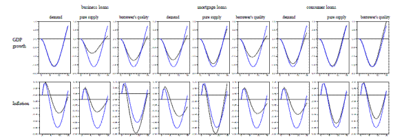
Figure 4C: Counterfactual analysis. Firm, household and bank balance-sheet channels in the Euro area. Responses of GDP growth and inflation to a monetary policy shock when closing down loan demand and loan supply (pure supply and borrower's quality) channels for each category of loans at a time.  18 figures of data plotted as curves, all with x-axis displaying quarters into future from 0 to 15, and y-axis displaying the response.  The figures are arranged into three six figures tables, one for business loans, one for mortgage loans, and the last for consumer loans.  Each table is composed of two rows and three columns, the top row for GDP growth, and the bottom row for inflation. The y-axis of figures on the GDP growth range from -2 to 2, and the inflation row has range of -0.3 to 0.1.  The columns represent demand, pure supply, and borrower's quality, in that order.  All figures in the GDP table have y-axis range of -0.5 to 0.5, and all figures in the inflation table have y-axis range of -0.2 to 0.2.  Each table arrangement has three columns and three rows.  The columns separate the type of loan: business loans, mortgage loans, and consumer loans, in that order.  Each panel has two curves: a blue curve representing the full system, and a black curve representing the correspondent channel being closed down.  

GDP growth response with the full system (blue curve): in all figures the curve is convex, decreasing to a minimum of about -1.5 at period 7.  The response becomes positive around period 13.  At period 15 the response is about 0.75.  

Inflation response with full system(blue curve): in all figures the curve begins as concave, increasing to a maximum of about 0.085 at period 2.  The response becomes negative around period 4, when the curve experiences an inflection point.  At period 9 the response reaches a minimum of about -0.25.  Around period 14 the response becomes positive, and around period 15 the response is about 0.03.  

First table, first column, first row: response with business loan demand and GDP growth.  The response closely follows the blue line response representing the full system.  First table, second column, first row: response with business loan pure supply and GDP growth.  The black line response is predominantly convex, falling to a minimum of about -0.75.  Around period 13 the responses cross, at a level very close to 0.  At period 15 the response is about 0.2.  First table, third column, first row: response with business loan borrower's quality and GDP growth.  The response is convex, falling to a minimum of about -1.2.  The responses cross around period 11 at a level of about -0.5.  At period 15 the black line response is slightly above 0.  First table, first column, second row: response with business loan demand and inflation.  The response begins as concave, reaching a maximum of about 0.08 at period 2.  The response then becomes negative around period 5, when there is also an inflection point.  The response falls to a minimum of about -0.15 at period 10.  The response crosses with the blue line response around period 13 at a level of about -0.08.  At period 15 the response is just below 0.  First table, second column, second row: response with business pure supply and inflation.  The response begins as concave, reaching a maximum of about 0.1 at period 2.  The response then becomes negative around period 5, when there is also an inflection point.  The response falls to a minimum of about -0.1 at period 10.  The response crosses with the blue line response around period 14 at a level just below 0.  First table, third column, second row: response with business loan borrower's quality and inflation.  The response begins as concave, reaching a maximum of about 0.08 at period 2.  The response then becomes negative around period 3, and there is an inflection point around period 5.  The response falls to a minimum of about -0.35 at period 9.  The responses never cross, and at period 15 the response is just below 0.  Second table, first column, first row: response with mortgage loan demand and GDP growth.  The response is convex, falling to a minimum of about -1.2.  The responses cross around period 12 at a level close to -0.5.  At period 15 the black line response is slightly above 0.  Second table, second column, first row: response with mortgage loan pure supply and GDP growth.  The response is convex, falling to a minimum of about -1.4.  The responses cross around period 12 at a level close to 0.  At period 15 the black line response is slightly above 0.5.  Second table, third column, first row: response with mortgage loan borrower's quality.  The response is convex, falling to a minimum of about -1.  The responses cross around period 12 at a level of about -0.2.  At period 15 the black line response is slightly above 0.  Second table, first column, second row: response with mortgage loan demand and inflation.  The response begins as concave, reaching a maximum of about 0.12 at period 2.  The response then becomes negative around period 5, when there is also an inflection point.  The response falls to a minimum of about -0.15 at period 10.  The response crosses with the blue line response around period 13 at a level of about -0.13.  At period 15 the response is about -0.08.  Second table, second column, second row: response with mortgage loan pure supply and inflation.  The response closely follows the blue line response for the full system, with the main difference being that the minimum is about -0.3, occurring at period 8.  Second table, third column, second row: response with mortgage loan borrower's quality and inflation.  The response begins as concave, reaching a maximum of about 0.1 at period 2.  The response then becomes negative around period 5, when there is also an inflection point.  The response falls to a minimum of about -0.12 at period 10.  The response crosses with the blue line response around period 14 at a level of about -0.08.  At period 15 the response is about -0.05.  Third table, first column, first row: response with consumer loan demand and GDP growth.  The response is convex, falling to a minimum of about -1.45.  The responses cross around period 12 at a level of about -0.75.  At period 15 the black line response is about 0.3.  Third table, second column, second row: response with consumer loan pure supply and GDP growth.  The response closely follows the blue line response representing the full system.  Third table, third column, first row: response with consumer loan borrower's quality and GDP growth.  The response closely follows the blue line response representing the full system.  Third table, first column, second row: response with consumer loan demand and inflation.  The response begins as concave, reaching a maximum of about 0.1 at period 2.  The response then becomes negative around period 5, when there is also an inflection point.  The response falls to a minimum of about -0.12 at period 10.  The response crosses with the blue line response around period 14 at a level of about -0.08.  At period 15 the response is about -0.05.  Third table, second column, second row: response with consumer loan pure supply and inflation.  The response closely follows the blue line response for the full system.  Third table, third column, second row: response with consumer loan borrower's quality and inflation.  The response closely follows the blue line response for the full system, with the difference being at the response reaches a minimum of about -0.17 at period 9.
Note: These graphs report counterfactual experiments. The responses of output growth and inflation to a one-standard deviation monetary policy shock are compared with the responses obtained when closing down the credit channels (one demand channel and two supply channels) for each type of loan at a time. The results of the full system (blue line) are compared with the results of the system where the correspondent channel has been closed down (black line). Responses of the series are normalised and divided by their innovation variances so that all responses to a shock are comparable on a single scale. All the responses refer to the Euro area. The panel VAR for the Euro Area is estimated assuming fixed effects, slope homogeneity and the country identification strategy as explained in Section 3. The specification of the VAR includes 12 variables: GDP growth, inflation, overnight rates, demand and supply (two channels) for all type of loans (see MODEL 4 in Section 3.5.) See Section 3 and Appendix for a detailed definition of the variables.

Figure 5A: Historical decomposition. The impact of different shocks during the financial crisis.

Figure 5A: Historical decomposition. The impact of different shocks during the financial crisis.
Figure 5a contains two panels, each of which is a bar graph with a single line graph drawn on top.  The x-axes go from the year 2007 to the year 2009, and the y-axes go from -5% to 1% for the top panel, and -3% to 1.5% for the bottom panel.  The bars in the charts represent the accumulated effects up to a time t of current and past innovations to other variables which explain movements in GDP growth. The black bar is for an own shock, the blue bar is for inflation, the green bar is for a loan demand from NFC, the red bar is for a loan demand for mortgages, the aqua bar is for the loan demand for consumer's credit, the pink bar is for the loan supply to NFC, the yellow bar is for the loan supply for mortgages, the grey bar is for the loan supply for consumer's credit, the orange bar is for monetary policy.  There is a brown line drawn over that represent GDP growth.
In the first panel, which is for the Euro area, in 2007Q3 the only bars that are visible are the black bar, which is just slightly negative with a value of roughly -0.2, the red bar which is just slightly positive with a value of 0.2, and the pink bar, which is negative with a value of -0.4. The GDP growth line starts at 0 and goes slightly negative to -0.25 over this quarter. In 2007Q4 the black bar is positive at 0.6, then red bar is positive at 0.2, the pink bar is negative at -0.5 and the orange line is 0.15. The GDP growth line is positive at around 0.3. In 2008Q1 the black bar is positive at 0.8, the blue, green, aqua and yellow bars are just a hair below zero, the red and grey bars are just a hair above zero, the pink bar is at -0.7, and the orange line is at about 0.2. The GDP growth line is positive but heading close to zero in this quarter.  In 2008Q2 the black bar is positive at 0.4, the blue, aqua and yellow bars are just slightly below zero, the red bar is at about -0.1, the pink bar is at -0.8, and the orange bar is positive at 0.4. The GDP growth line is becoming increasing negative in this quarter at about -1%. In 2008Q3, the black bar is negative at -1 and the pink bar is also negative at -0.8. The green, aqua and yellow bars are slightly negative, the red bar is negative at 0.3, the grey bar is slightly positive and the orange bar is positive at 0.5. The GDP growth line continues to become rapidly more negative in this quarter. In 2008Q4, the black bar is much more negative at -3.5 (though still above the GDP growth line), the blue bar and grey bars are slightly above zero, the aqua and yellow bars are slightly below zero. The green bar is negative at -0.2, the red bar is negative at -0.5, the pink bar is negative at -0.9 and the orange bar is positive at 0.6. The GDP growth line at this point is far below all the bars at about -4 and continuing to decrease.  In 2009Q1, the black bar is very negative at -3.4, the blue bar is slightly positive at 0.1, the green bar is negative at -0.2, the red bar is negative at -0.5, the aqua bar is virtually zero, the pink bar is negative at -0.7, the yellow bar is slightly negative, the grey bar is slightly positive, and the orange bar is positive at 0.8. The GDP growth line is still around -4% in this quarter but is starting to increase again.

In the second panel, which is for the US, in 2007Q3 the only bar that is visible is the black bar, which is at 0.9, and the GDP growth is at the same value and gently sloping down. In 2007Q4, the black bar is at 0.7, the blue and grey bars are slightly above zero at 0.05, the green, aqua, pink and yellow bars are just a hair below zero. The GDP growth line has a slight dip in this quarter before heading up again. In 2008Q1 the black bar is at 1.3, the blue and pink bars are just slightly above zero, the blue, yellow and green lines are just slightly below zero, and the grey bar is at 0.1. The GDP growth line is at around 1% and slightly increasing in this quarter. In 2008Q2 the black bar is at 1.4 (above the GDP growth line), the blue and grey bars are positive at 0.01, the aqua bar is slightly above zero, the green and pink bars are at about -0.01 and the yellow bar is at about -0.25. The GDP growth line is decreasing from about 1%. In 2008Q3, the black bar is positive at 0.75, the blue bar is positive at 0.25, the green, red, aqua and pink bars are all just below zero, the grey bar is negative at -0.15 and the yellow bar is at -0.5. The GDP growth line is crossing the y-axis at this point and decreasing.  In 2008Q4, the black bar is positive at -0.4 and the orange bar is just a hair above zero.  The green, red and aqua bars are all at about -0.15, the pink bar is at -0.5, the yellow bar is at negative -0.9, and the grey bar is at -0.2. The GDP growth line is at about -1.5% and still decreasing.  In 2009Q1 the black bar is at negative -1.2, the yellow bar is at -2.2, the pink bar is at negative -0.5, the grey bar is at negative -0.2, the blue, green and red bars are slightly just below zero and the orange bar is just above zero. The GDP growth line is still decreasing when it ends at -2.5.
Note: These graphs report the results of a historical decomposition. The decomposition is technically performed by estimating the VAR model until the beginning of the financial crisis (2007Q2), projecting the variables of interest over the crisis sample (2007Q3 - 2009Q2) and decomposing the difference between the realised and the projected values in the sum of the innovations to all variables. The bars in the charts represent the accumulated effects up to time t of current and past innovations to other variables which explain movements in GDP growth. All types of loans are considered for the Euro area and for the United States (US). The panel VAR for the Euro Area is estimated assuming fixed effects, slope homogeneity and the country identification strategy as explained in Section 3. The specification of the VAR includes 9 variables: GDP growth, inflation, overnight rates, demand and supply for business loans (loans to NFC), mortgage loans and consumer loans (see Model 2 in Section 3.5). See Section 3 and Appendix for a detailed definition of the variables.

Figure 5B: Historical decomposition. The impact of different shocks during the financial crisis (bank lending and borrower's balance sheet channels)
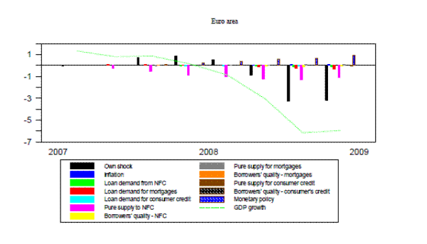
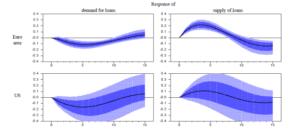
Figure 5B: Historical decomposition. The impact of different shocks during the financial crisis (bank lending and borrower's balance sheet channels)
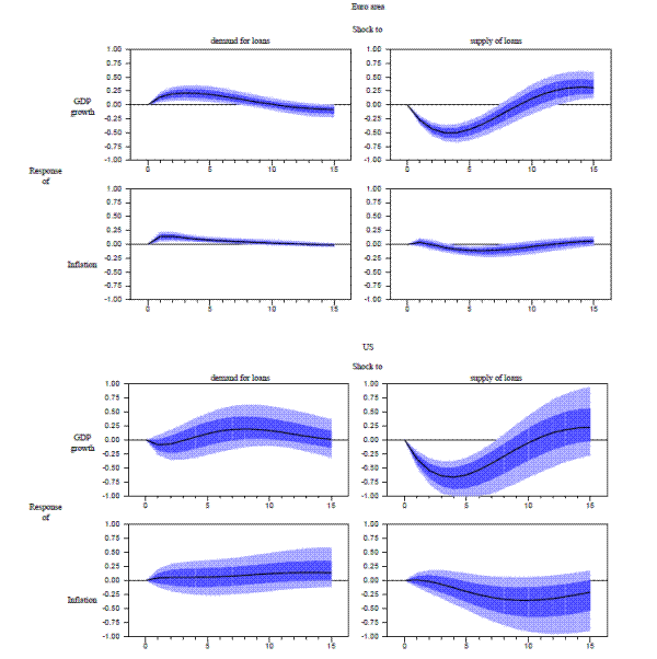
Figure 5B contains a bar graph with a single line plot drawn on top and it is labeled &quote;Euro area&quote;. The x-axis goes from the year 2007 to 2009, and the y-axis goes from -7% to 2%.  The bars in the charts represent the accumulated effects up to a time t of current and past innovations to other variables which explain movements in GDP growth. The black bar is for an own shock, the blue bar is for inflation, the green bar is for a loan demand from NFC, the red bar is for a loan demand for mortgages, the aqua bar is for the loan demand for consumer credit, the pink bar is for the loan supply to NFC, the yellow bar is for the loan supply for mortgages, the grey bar is for the loan supply for consumer's credit, the orange bar is for monetary policy, the born bar is for pure supply for consumer credit, the checkered black bar is for borrower's quality-consumer's credit, and the checkered blue bar is for monetary policy.  There is a green line drawn over that represents GDP growth.
In the first period of the graph, in 2007, there is only the black bar that is very slightly negative.   The green line is at about 1.5 and slowly declining.
In the second period of the graph, there is the red bar with is slightly positive, and the pink bar which is slightly negative at about -0.25.  The green line is at 1.
In the third period, the black bar is positive at 1, the pink bar is negative at -0.75, and red, orange, and checkered blue bars are all very slightly positive. The green line remains at one.
In the fourth period, the black bar is positive at 1.25, the pink bar is negative at -1, and red bar is slightly positive. The green line is at about 0.5 and is declining.
In the fifth period, which is at 2008, the checkered blue bar is at 0.25, the black bar is at 0.75, the pink bar is at -1.25, and the grey bar is just slightly above zero. The green line is negative and at about -1, declining more rapidly.
In the sixth period, the checkered blue bar is at about 0.5, the black bar is at -1, the green, orange and red bars are slightly negative, and the pink bar is negative at -1.25. The green line is at -3 and continuing to decline.
In the seventh period, the checkered blue bar is at 0.75, the black bar is at -3, the yellow, blue and grey bars are slightly above zero, the green bar and red bars are slightly below zero, and the pink bar is at -1.5. The green line is at -5 and continuing to decline.
In the eighth period, the black bar is at -2.75, the pink bar is at -1.25, the grey and blue bars are slightly above zero, the green bar is slightly below zero, the red bar is at -0.5 and the checkered blue bar is at 1. The green line is at -6 and is slowly increasing.
Note: These graphs report the results of a historical decomposition. The decomposition is technically performed by estimating the VAR model until the beginning of the financial crisis (2007Q2), projecting the variables of interest over the crisis sample (2007Q3 - 2009Q2) and decomposing the difference between the realised and the projected values in the sum of the innovations to all variables. The bars in the charts represent the accumulated effects up to time t of current and past innovations to other variables which explain movements in GDP growth. Only the Euro area and all types of loans are considered. The panel VAR for the Euro Area is estimated assuming fixed effects, slope homogeneity and the country identification strategy as explained in Section 3. The specification of the VAR includes 12 variables: GDP growth, inflation, overnight rates, demand and supply (pure supply and borrower's quality channels) for business loans (loans to NFC), mortgage loans and consumer loans (see Model 4 in Section 3.5). See Section 3 and Appendix for a detailed definition of the variables.

Footnotes

* We are grateful to Egon Zakrajsek for providing us with some of the data from the Senior Loan Officer Survey and to Francesca Fabbri for her excellent work as research assistant. We also thank Gabriel Fagan, Hanna Hempell, Michele Lenza, Jesper Lindé, Simone Manganelli, Eva Ortega, Huw Pill, Frank Smets, Ilya Strebulaev and all the participants to the Bank of Italy seminar, the ECB internal seminar, the CREDIT conference in Venice, and the workshop "Financial Markets and the Macroeconomy: Challenges for Central Banks" in Stockholm for useful suggestions and comments. Any remaining errors are our responsibility. The views expressed are our own and do not necessarily reflect those of the European Central Bank or the Eurosystem. Email contacts: [email protected], [email protected], and [email protected]. Return to Text
1. The available empirical evidence on the bank lending channel is not conclusive, and comprises both works supporting the bank lending channel (e.g., Kashyap and Stein, 2000; Peek and Rosengren, 1995, 1997), and works finding evidence in favour of a more conventional transmission mechanism (Romer and Romer 1990; Ramey 1993). For an exaustive and recent review of the empirical evidence on the transmission mechanism see Boivin, Kiley and Mishkin (2009). Return to Text
2. The available information related to the factors affecting banks' decisions is more comprehensive in the Euro area BLS. Return to Text
3. For the sake of symmetry we consider the federal funds rate as the measure of monetary policy for the U.S., though the actions by the Federal Reserve in the current crisis were directed towards several markets and implemented through several different mechanisms (Bernanke, 2009, and ECB, 2009). Hence, for the U.S. the overnight rates may not be a complete measure of monetary policy stance. However, the main results we present in the paper are robust to considering the period up to September 2008. Return to Text
4. Lown and Morgan (2006) also analyze the information content of the SLO. However, they use only the answers from one of the questions of the survey on lending standards - namely changes in credit standards applied to C&I loans - and proxy loan demand by macro variables commonly used in the literature. Since they want to analyse the predictive power of lending standards, they use the whole history of the SLO survey and don't include the answers to questions related to the loan demand, which only started in 1991. They find that the credit standards predict future output and credit growth. Our work is distinct from their analysis in the objective that we want to achieve and in the analysis that we implement. Our objective is to test the credit channel of monetary policy. To this aim, we use several answers from the bank lending survey to fully exploit the information content. The survey includes questions on the factors behind the decision to change lending standards. We exploit this information and also the answers related to the loan demand. Return to Text
5. See Lown and Morgan (2006) and De Bondt et al. (2009) for the respective predictive power of the surveys for output and credit growth in U.S. and the Euro area. Return to Text
6. Berg, van Rixtel, Ferrando, de Bondt and Scopel (2005) describe in detail the setup of the survey. Sauer (2009) and Hempell, Köhler-Ulbrich and Sauer (2009) provide an update including the most recent developments and the few changes implemented (request of additional information via ad-hoc questions). The survey was first used for research purposes in Maddaloni and Peydro (2009) and Maddaloni, Peydro and Scopel (2008). Return to Text
7. The Euro Area financial system is bank dominated, as shown by Maddaloni et al. (2004). Return to Text
8. This classification is somewhat different from the classification used in the US for the Senior Loan Officer Survey where mortgage loans are further disentangled in prime and subprime loans. Return to Text
9. As we have access to information on banks' size, an interesting hypothesis stemming from the bank lending channel is that the credit channel should be stronger for small banks. We postpone this analysis to future investigation. Return to Text
10. At the start, there were 87 banks answering the survey. This figure remained almost fixed until 2007, when Slovenia entered the euro area and Slovenian banks entered in the survey. Successively, in 2008, this figure reached 112 with the inclusion of Cyprus, Malta and an enlarged sample for Italy and Germany. Return to Text
11. The factors that change loan demand also contain some useful information. An interesting hypothesis to check in future is whether the economic impact of the credit channel is stronger when loan demand increases, given the lack of access to other financing sources. Return to Text
12. In cases when foreign banks are part of the sample, the credit standards refer to the loans' policy in the domestic market which may differ from guidelines established for the headquarter bank. Return to Text
13. The answers related to the factors which changed the lending standards applied by banks (i.e. why banks have tightened lending standards) further strengthen the identification of loan supply restrictions. These factors can be categorized in two main groups: (1) factors linked to the ability of banks to lend in relation with their balance sheet constraints and the competitive pressures; (2) factors linked to changes in borrowers' risk. In our setting the answers related to the first group of factors identifies "pure (loan) supply" restrictions and, therefore, the bank lending transmission channel. This information is useful not only to disentangle the bank lending channel from the firm/household channel, but also to strentghten the loan supply identification (over and above loan demand volume and quality). Return to Text
14. The series on lending standards for large and small enterprises have a correlation of 96%. The series on demand for loans from large and small enterprises have a correlation of 93%. For the Euro Area the general question on firms refers to all firms, but then one of the secondary questions refer to lending standards applied to large versus SME firms. Return to Text
15. This information can be interpreted as a direct measure of banks' appetite for risk in lending behaviour in the US. While the BLS for the Euro Area does not provide directly a measure for banks' risk appetite, the richness of survey information allow to extract this measure indirectly by controlling for the other factors and by analysing the terms and conditions of the loans (see Maddaloni and Peydró, 2009). Return to Text
16. In addition, some of the questions about the factors affecting changes in lending standards were added only in recent years, which further restrict the use of these answers over the entire time series for the SLO. Return to Text
17. Questions related to the demand for consumer loans were included only in 1995Q4. Return to Text
18. The use of this statistic implies that no distinction is made for the degree of tightening (easing) of lending standards in the replies (similarly on the degree of increase in the demand for loans). This issue can be addressed using diffusion indexes. A simple way of calculating these indexes consists for example in weighting by 0.5 the percentage of banks answering that they have tightened somewhat (eased somewhat) and in weighting by 1 the percentage of banks that have tightened considerably (eased considerably). A similar weighting scheme can be applied to the answers concerning demand for loans. The results obtained using diffusion indexes do not differ qualitatively from the results obtained with net percentages and, therefore, we do not report them since they also imply a certain level of discretion when choosing the weights. Return to Text
19. For the US SLO it is not possible to do all these correlations for household loans. For the Euro Area results are similar for loans to households. Return to Text
20. Even though there is no official CEPR dating of the Euro Area business cycle after the 1990s, the Euro Area four-quarter growth rates of GDP shows the features of a complete cycle from 2002 to 2008. Heterogeneity across countries are nevertheless sufficient to ensure reliable estimates from a panel strategy, while ex-post tests do not reject our common slope assumption in the panel. Hence, there is enough heterogeneity in the Euro Area to exploit a panel but not so much that prevents pooling. Return to Text
21. Note that Model 4 is estimated only for the Euro Area, whereas for the U.S. we limit our extended analysis to Models 2 and 3 as the US SLO does not dispose of all the needed detailed information. Return to Text
22. The choice of this ordering is especially justifiable in the Euro Area, where the monetary policy strategy is based on a two-pillar approach and explicitly takes into account information from credit aggregates. Return to Text
23. The results for the US are similar to Lown and Morgan (2006). Return to Text
24. A one-standard deviation shock corresponds to an increase of the short-term interest rate of around 60 basis points in the U.S. and of 30 basis points in the Euro area. Return to Text
25. The blue lines are the responses in a system where all the channels are active. The black lines are computed from a system where the supply or demand channel has been closed down, i.e. where coefficients of supply or demand in all equations have been set to zero. Return to Text
26. As before, the black lines are computed from a system where the supply or demand channel has been closed down, i.e. where coefficients of supply or demand in all equations have been set to zero. Return to Text
27. The decomposition is technically performed by estimating the VAR, projecting the variables of interest over the crisis sample (2007Q3-2009Q2), and decomposing the difference between the realised and the projected values in the sum of the innovations to all variables. See, e.g. Doan (2009) for more details. Return to Text
28. As explained in Section 3.4 the level of EONIA rate embeds also the effect of the full allotment policy. Return to Text

This version is optimized for use by screen readers. Descriptions for all mathematical expressions are provided in LaTex format. A printable pdf version is available. Return to Text