Skip to: [Printable Version (PDF)] [Bibliography] [Footnotes]

Finance and Economics Discussion Series: 2007-52 Screen Reader version

Do High Debt Payments Hinder Household Consumption Smoothing?

Kathleen W. Johnson

Geng Li

Board of Governors of the Federal Reserve System¹

July 2007

Keywords: Household debt, consumer finance, consumer spending

Abstract:

Over the past fifteen years, U.S. households have committed a rising share of their disposable personal income to required principal and interest payments on household debt. The direct link between the household debt service ratio (DSR) and consumption has been studied in the literature, but the results of these studies are mixed--perhaps because debt may not have a direct effect on consumption growth, but rather may alter the relationship between consumption and income. We explore this possibility by comparing the consumption smoothing behavior of households in the 1992 to 2005 waves of the Consumer Expenditure Survey over the DSR distribution. Our approach has two advantages relative to the existing literature. First, it avoids the most obvious source of endogeneity between debt and spending. Second, this approach is to our knowledge the first serious look at household-level DSRs. We find that a high DSR alone does not indicate higher sensitivity of consumption to a change in income. However, we find evidence that the DSR may help identify borrowing constrained households. In particular, the consumption of households with low liquid assets and high DSRs is more sensitive to income changes than the consumption of other low liquid asset households. Although the effect of a higher DSR is not precisely estimated, it is large and robust to changes in the specification, suggesting that more work is warranted.

Introduction

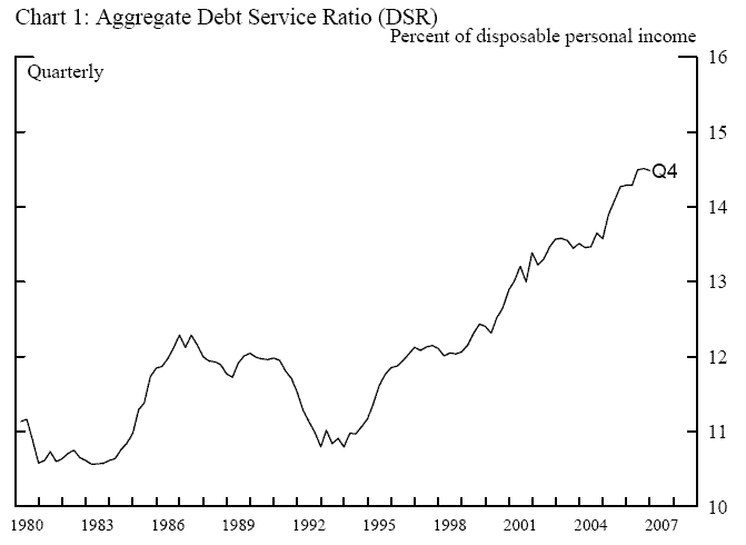
Over the past fifteen years, U.S. households have committed a rising share of their disposable personal income to required principal and interest payments on household debt such as mortgages, automobile loans and credit card balances. This share, also known as the debt service ratio (DSR), equaled 14 percent at the end of 2006, 3 percentage points higher than it was at the end of 1991 (chart 1). What may have caused this rise and what are the potential consequences? The DSR rose in part because net declines in interest rates over this period spurred the demand for debt, which all else equal will raise the DSR.² In addition, the increase in the DSR may reflect the extension of mortgage and consumer credit to households who could not previously qualify (Johnson, 2005; Dynan, Johnson and Pence, 2003; Bostic, 2002). Also, the increase in the DSR may reflect changes in the credit card market. As more households use their credit cards as a convenient payment method, the increase in short-term, interest-free loans associated with convenience use may increase the DSR (Johnson, 2007). A more comprehensive and thorough enumeration of these causes can be found in Dynan and Kohn (2007).

This rise in the DSR has generated interest of late because it could potentially cause households to cut back spending. This hypothesized link has been studied in the literature, but the results of these studies are mixed. Some researchers examined the link between aggregate household debt and consumption (Bachetta and Gerlach, 1997 and Ludvigson, 1999) and found that a rise in the growth of household debt raises the growth of consumption. However, over a more recent time period, Johnson (2007) found that a rise in the growth of revolving consumer debt reduces the growth of consumption. Other researchers focused on the link between aggregate payments on debt and consumption. Mishkin (1976) and McCarthy (1997) find that a rise in debt payments leads to lower expenditures on durable goods, but McCarthy (1997) and Maki (2002) conclude that it does not lead to lower overall spending. Finally, some looked at this link at the household level, studying the effect of exogenous changes in debt payments on household consumption, but this work as a whole is inconclusive. Stephens (2005) concludes that non-durable expenditures respond to the repayment of a vehicle loan, whereas Coulibaly and Li (2006) conclude that only durable goods expenditure--such as household furnishings--respond to the repayment of a mortgage loan.

One reason for these seemingly contradictory results may be that debt does not have a strong, direct effect on consumption growth, but rather may alter the relationship between consumption and income. In this paper, we explore this possibility by comparing the consumption smoothing behavior of households across the distribution of their DSRs. Importantly, this paper does not attempt to test whether household consumption is excessively sensitive to changes in income, relative to the predictions of the permanent income hypothesis. Rather, we take the degree of consumption smoothing observed in the data as given and ask whether a high DSR hinders a household's ability to smooth through income fluctuations relative to a low DSR. To answer this question, we use the 1992 to 2005 waves of the Consumer Expenditure Survey (CEX). The CEX contains comprehensive data on household-level consumption supplemented with information on household balance sheets.

Our approach has two advantages relative to the existing literature: First, because household credit is used to finance consumption, credit and consumption are jointly determined. Previous studies of the relationship between aggregate credit and consumption generally addressed endogeneity with instrumental variables; studies at the household level viewed the maturing of a loan as a plausibly exogenous source of debt payment variation. Our approach avoids this most obvious source of endogeneity by studying the indirect effect of the DSR on the ability to smooth consumption through income fluctuations.

Second, to our knowledge, this approach is the first serious look at household-level DSRs, which vary substantially both across time and households. Although the average DSR in our data fluctuates no more than the aggregate DSR, this smoothness masks a considerable amount of heterogeneity. This cross-section variation provides better identification than regressions using aggregate data and permits us to control for a variety of household characteristics. Also, by looking at the effect over different groups of households, we can better understand the relationship between household debt and consumption. Our results indicate that households with relatively high DSRs are no less able to smooth through income fluctuations than other households. This may in part reflect the higher level of liquid assets that high DSR households appear to hold.

Related Literature

The literature to date presents mixed evidence about the link between household debt and consumption. Some studies have found a relationship between particular measures of debt and particular measures of consumption. Others have found no relationship at all. This literature has generally taken one of three perspectives.

The first set of papers took an economy-wide perspective and involved regressions of growth in various measures of aggregate consumption on the expected growth in various measures of aggregate household debt. Bacchetta and Gerlach (1997) observed that expected growth in mortgage and consumer credit, as well as the wedge between borrowing and lending rates in the United States, are positively correlated with the growth in nondurable goods and services expenditures. They suggest that consumption therefore plays an important role in the transmission of monetary policy because it is influenced by the cost and availability of credit. Similarly, Ludvigson (1999) discovered that a 1.0 percentage point rise in anticipated consumer credit growth is correlated with a 0.1 percentage point rise in the growth of nondurable goods and services expenditures. She also demonstrates how her finding may be consistent with significant variation in consumer credit ceilings. On the other hand, McCarthy (1997) found only a negligible link between household credit and nondurable goods and service expenditures, but a more significant link between credit and durable goods expenditures. Johnson (2007) also observed a negligible link between household credit and total expenditures, and a negative link between growth in credit card debt and total household expenditures.

The second set of papers also took an economy-wide perspective, but focused on debt payments rather than levels of debt. The conclusions of these papers more consistently show that debt payments influence expenditures on durable goods, but these effects are not large enough to show through to overall spending. Maki (2002) ascertained that the DSR does not add information to a model of the growth of consumption that includes past growth of consumption, the growth of income, wealth and the real federal funds rate as regressors. McCarthy (1997) learned the DSR does enter significantly into a similar model of the growth in expenditures on durable goods. In this specification, a 1.0 basis point rise in the DSR leads to a 5 basis point decline in the annual rate of growth in durable goods expenditures in the following period. Mishkin (1976) also finds a negative relationship between consumer liabilities and durable expenditures in a stock adjustment model.

The final perspective taken in the literature is that of the individual household, and here the evidence is more mixed. Stephens (2005) found that "a 10 percent increase in discretionary income due to the final repayment of a vehicle loan increases non-durable consumption by 2 to 3 percent."³ In contrast, Coulibaly and Li (2006) observe that households do not increase their non-durable consumption following the retirement of their mortgage, but do increase durable goods consumption, such as home furnishings and entertainment equipment.

The evidence in the literature to date not only fails to reach a consensus, but is hard to interpret because of the number of different ways debt payments may affect consumption. Five channels through which debt payments may be linked to consumption are summarized in table 1. First, interest rates help jointly determine both debt payments and consumption. When interest rates fall, households borrow more to pull forward a portion of future consumption. Current consumption increases relative to past consumption and debt payment rises, creating a positive relationship between current consumption growth and debt payments. For a given level of debt, a fall in the interest rate will also reduce the debt payment, but considering the maturity of most household loans, this effect is small relative to the effect of a rise in debt on payments.

Second, debt payments may be correlated with household consumption because they are an indicator of expected future income growth. As households learn that their future income has risen, they will raise current consumption relative to past consumption and are more willing to commit themselves to future debt repayment. Under this hypothesis, the relationship between current consumption growth and debt payments is also positive.

The next channel relates to durable goods. A rise in a household's debt payments raises the probability that a household will find itself in financial distress and need to sell its durable good assets for less than their full value. Thus, households with higher debt payments should be less willing to hold durable goods and more willing to hold liquid financial assets, creating a negative relationship between debt payments and growth in future durable goods expenditures. Also, many households finance durable goods purchases with consumer credit, which allows households to better match the payment stream for these durables with the consumption of their services. Because durable goods purchases are lumpy, a surge in expenditures in one period, which in turn leads to higher debt payments, will likely result in a decline in expenditures in the following period. Thus, under this hypothesis, debt payments and subsequent growth in durable goods expenditures are negatively related.

In the final channels, household debt payments may also be correlated with household consumption because some households are borrowing constrained. Borrowing constraints, as it has been argued, can create either a positive or a negative relationship between the DSR and consumption growth. Across households, those who are borrowing constrained will have higher consumption growth and lower debt than those that are not borrowing constrained, creating a negative relationship between debt payments and consumption growth. In contrast, over time, a rise in the DSR may suggest a relaxation of credit constraints so that some households can increase their consumption more than in the past. This implies a positive relationship between changes in debt service and consumption growth.

Table 1: Channels through which Consumption and the DSR may be related

Channel	Relevant relationship	Sign
Interest rates	Current consumption growth and DSR	Positive
Expectations of future income	Current consumption growth and DSR	Positive
Durable goods	Current consumption growth and lagged DSR	Negative
Liquidity constraints: Binding	Current consumption growth and DSR across households	Negative
Liquidity constraints: Relaxation of	Current consumption growth and change in DSR over time	Positive

Rather than attempt to reconcile these disparate findings, we will take a perspective not yet addressed in the literature. We will explore the possibility that debt payments may not have a direct effect on consumption growth, but rather may alter the relationship between consumption growth and income growth. Specifically, we ask whether a high DSR hinders a household's ability to smooth through income fluctuations relative to a low DSR.

Before we study this relationship in detail, we discuss the quality of our household-level measure of debt service and ask whether the increase in the debt service ratio over the period covered by our micro-data was broad-based.

A Household-level Measure of Debt Service

Measurement of Debt Payments in the Consumer Expenditure Survey (CEX)

We use the 1992 to 2005 waves of the CEX for our study. The CEX has been conducted consistently since the early 1980's by the Bureau of Labor Statistics to provide weights for the market basket used to construct the Consumer Price Index. As part of its expenditure data collection, the BLS asks households to report its payments on household debt, including mortgages, vehicle loans and other consumer debt, which will make up the majority of debt payments in our measure. Mortgage debt payments accounts for close to 60 percent of total debt payments, vehicle debt accounts for about 20 percent and the remainder is accounted for by credit card debt.

As noted by the BLS, "consumer expenditure surveys are specialized studies in which the primary emphasis is on collected data related to family expenditures for goods and services used in day-to-day living." (BLS 2006) As such, many studies validating the CEX data focused on its ability to replicate aggregate measures of consumption, such as personal consumption expenditures (PCE) reported quarterly by the Bureau of Economic Analysis (BEA). In general, these validation studies (see for example, Gieseman, 1987; Branch, 1994) conclude that aggregate expenditures reported in the CEX are below those reported by the BEA.

Although validation studies have been conducted on the consumption data in the CEX, we are unaware of any study that validated the CEX liability data. Thus, before proceeding, we compare household debt payments measured in the CEX with that measured in the Survey of Consumer Finances (SCF). The SCF is a triennial survey conducted by the Federal Reserve System that collects high-quality data on household wealth holding and debt balance and payments as well as very rich covariates such as household demographics and income data. We presume the accuracy of the SCF data and compare its debt payment information with that of the CEX. In general, this exercise has increased our confidence that debt payments for the major types of household debt are measured reasonably well in the CEX.

Debt payments in the CEX and the SCF

Many of the types of debt covered by the CEX have similar counterparts in the SCF. Both the CEX and the SCF report payments on first mortgages, home equity loans and lines of credit on the household's primary residence. However, for debt collateralized by other properties, the SCF reports only total payments, while the CEX breaks these payments down by loan type (first lien, home equity loan, etc.). Both the CEX and the SCF includes payments on vehicle loans, and the amount of credit card debt, which can be used to estimate its required monthly payment.⁴ Finally, for other types of loans, the CEX reports only total payments on "other personal loans", whereas the SCF provides more detail, breaking payments down by loan type (student loans, installment loans, other lines of credit and personal loans). Because it is difficult to reconcile both the concept and measurement of the "other loans" category between the two surveys, we include only payments on loans secured by real estate and automobiles, and credit card loans in our measure of debt payments. Table 2 lists the categories of debt from the SCF and the corresponding UCC codes in the CEX used to construct total debt payments.

Table 2: Summary of Debt Payment Variables in the SCF and CEX

SCF Debt Payment Categories	Corresponding CEX UCC Code
1. Primary residence mortgages	220311, 830201
2. Other Real Estate Real Estate Backed Loans
2. A. Home equity loans secured by primary residence	220313, 830203
2. B. Lines of credit secured by primary residence	880110, 880120
2. C. Mortgages, home equity loans and lines of credit on vacation homes and other properties	220314, 790940, 830204, 220312, 790920, 830202, 880120, 880210, 880220, 880310, 880320
3. Vehicle loans	850100, 870103, 870203, 870803
6. Credit cards	Not computed using UCC level data
7. Other consumer loans	Not comparable

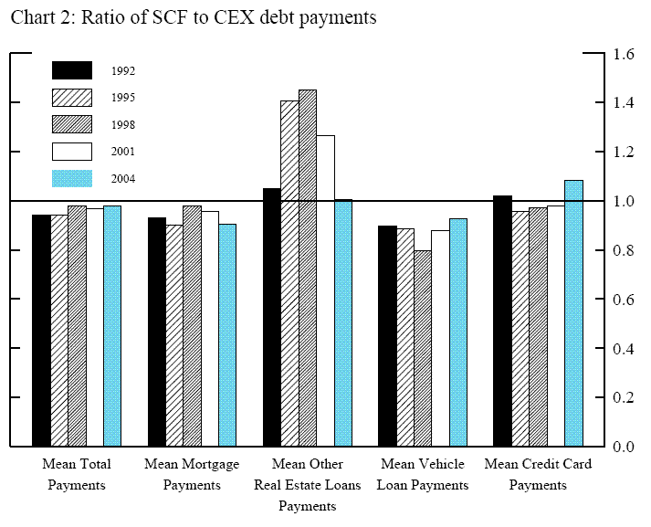
Broadly speaking, the level of total household debt payments for these three types of debt calculated from the CEX sample lines up fairly well with that calculated from the SCF sample (chart 2).⁵ For each wave of the SCF from 1992 through 2004, the mean of total household debt payments calculated from the CEX sample is within about 5 percent of the mean from the SCF sample for the corresponding year, with an average gap over the five SCF waves of about 3 percent.⁶

Much of the accuracy in the CEX data reflects mortgage payments on primary residences; on average over the four SCF waves, the mean of debt payments on primary residence mortgages calculated from the CEX sample is within 6 percent of that calculated from the SCF sample. The SCF data, in turn, aligns closely with that from the Residential Finance Survey, a survey in which chosen households are required by law to participate and incorporates information from lenders (Bucks and Pence, 2006). This alignment strongly suggests the mortgage payment data in the CEX are reported accurately.

Loans for real estate other than the household's primary residence and for automobiles align less closely between the CEX and SCF. The gap between loans for other real estate calculated from the CEX and that calculated from the SCF is about 22 percent, but payments on these loans account for only about 10 percent of total payments. The gap between payments on automobile loans measured by the two surveys, which account for about 20 percent of total payments, is only about 12 percent. Finally, minimum required payments on credit cards are closely aligned between the two surveys, with a gap of less than one percent over the five waves of the survey.⁷

Debt payments measured by the CEX sample also display patterns across demographic groups similar to patterns in debt payments measured by the SCF sample. Many of these differences across demographic groups mirror those of household income. Total debt payments in the CEX rise with the age of the household head until around age 45 and then fall steadily--a pattern mimicked by nearly all types of debt (table 3). Households whose head is white have higher debt payments on average than those whose head is nonwhite. Debt payments also rise with education--households whose head has at least a college degree had about 3 times more debt payments than those whose household head has less than a high school diploma. Finally, married households had over twice the debt payments of unmarried households. Each of these patterns is also evident in debt payments measured by the SCF sample.

Table 3: Debt Payments, by demographics and household survey

	Total Debt Payments: SCF	Total Debt Payments: CEX	Mortgage: SCF	Mortgage: CEX	Other Real Estate: SCF	Other Real Estate: CEX	Vehicle: SCF	Vehicle: CEX	Credit Card: SCF	Credit Card; CEX		Total Debt Payments: SCF	Total Debt Payments: CEX	Mortgage: SCF
Age 35	7,093	7,863	3,879	4,634	544	344	2,071	2,260	599	625	Age 35	7,093	7,863	3,879
35 - 45	11,452	12,073	7,705	7,961	717	810	2,329	2,664	701	638	35 - 45	11,452	12,073	7,705
45 - 55	12,002	11,392	7,912	7,256	1,432	1,120	2,021	2,237	637	779	45 - 55	12,002	11,392	7,912
55 - 65	9,441	9,652	5,639	5,739	1,858	1,414	1,437	1,954	508	546	55 - 65	9,441	9,652	5,639
65 - 75	5,453	5,210	3,226	3,461	1,098	513	670	953	459	284	65 - 75	5,453	5,210	3,226
Age 75	1,350	2,676	711	1,924	232	127	303	399	104	226	Age 75	1,350	2,676	711
White	9,374	9,265	5,932	5,873	1,130	803	1,740	2,009	571	581	White	9,374	9,265	5,932
Nonwhite	6,295	5,952	3,759	3,523	468	463	1,578	1,469	490	497	Nonwhite	6,295	5,952	3,759
Lower than HS	3,001	3,720	1,679	2,300	231	163	913	1,013	178	243	Lower than HS	3,001	3,720	1,679
HS	6,373	7,164	3,536	4,166	626	718	1,703	1,814	508	467	HS	6,373	7,164	3,536

Overall, debt payments in the CEX appear to be fairly accurately measured relative to those in the SCF, with debt payments for primary mortgages and for credit cards the most similar between the two surveys and those for mortgages on other real estate and automobile loans less similar. Based on this evidence, we conclude that our results should be broadly representative for the U.S. population as a whole over the period 1992 to 2005. A limitation of the study is that we do not have information after 2005, a period of some notable developments in household borrowing.

The Time Trend in CEX Debt Payments

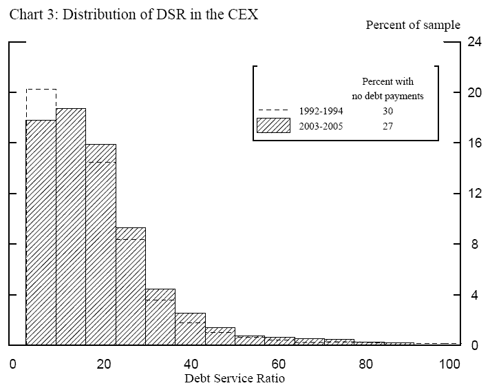
In the aggregate, the DSR rose significantly over the period covered by our survey data. Consistent with this rise, the distribution of the DSR shifted to the right during this time (chart 3). As shown in the inset, the share of households with no debt payments has declined a bit. In addition, as can be seen, there is considerable heterogeneity across households, which will help us identify the effect of the DSR on households' sensitivity to income fluctuations.

We are interested in whether this rightward shift reflects a broad-based increase in debt service, or whether it indicates as significant rise among a select group. For example, the shift in the DSR may have been related, in part, to a rise in homeownership, and the associated rise in the share of households with mortgage payments. The CEX data show that the share of households with mortgage payments increased from about 45 percent of households in the earlier years of our sample to about 51 percent in recent years. 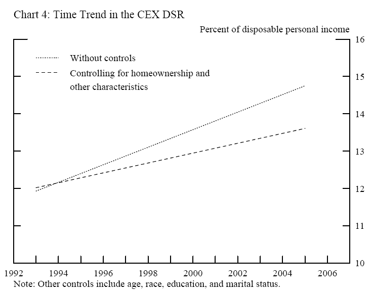To take a closer look at the influence of the rise in homeownership, along with changes in other household characteristics, on the DSR, we regressed the household-level DSR from the CEX on year dummies and compare the trends from regressions with and without homeownership and other household characteristics as control variables, shown in equation 1.

$$\left( 1 \right)\quad DSR_i =\alpha _0 +\alpha _1 time+\alpha _2 x_i ,$$

where is a vector that includes homeownership, age, education, marital status and race.

The dotted line in chart 4 shows the smoothed time trend in the household-level DSR without controlling for household characteristics.⁸ The uptrend is broadly similar to that of the aggregate DSR over the same time period. After controlling for household characteristics--indicated by the dashed line--the slope is substantially reduced but still significantly upward. All told, the remaining significant upward trend suggests that some part of the rise in the aggregate DSR over time reflects a broad trend towards higher debt service across all types of households. We now turn to how to interpret the effect of this broad trend on household spending.

Conceptual Framework and Model Specification

Our framework for analyzing the effect of debt service on consumption smoothing is a standard model of the sensitivity of consumption to income changes. Assume households maximize the expected discounted sum of lifetime utility,

$$\begin{array}{l} (2)\mbox{ }\max E\sum\limits_{t=0}^\infty {\delta ^t} U(C_t ,\mbox{ }\theta _t ) \ \ \end{array},$$

subject to the constraint

$$\mbox{(3) }A_{t+1} =A_t (1+r)+Y_t -C_t \quad \quad -\infty <A_t <+\infty ,$$

and a transversality condition

$$\mbox{(4) }\mathop {\lim }\limits_{T\to \infty } A_T \ge 0,$$

where 1 is the discount factor, is period t consumption, is a scalar function of a household demographic characteristics vector that would affect the marginal utility, is net assets, which are negative if the household is a net borrower, and is labor income. Further assume that households have constant relative risk aversion (CRRA) preference and the utility function is given by

$$\begin{array}{l} (5)\mbox{ }U(C_t ,\mbox{ }\theta _t )=\frac{C_t ^{1-\rho }}{1-\rho }\times e^{\theta _t } \ \ \end{array},$$

In an economy with complete information and perfect financial markets, the first-order condition of households can be written as the Euler equation

$$\begin{array}{l} \mbox{(6) }\Delta \log (C_t )=\beta _0 +\beta _1 \mbox{ }\Delta \theta _t \ \ \end{array},$$

where and are linear functions of the parameter in equations (2) - (5). Although these assumptions imply that consumption growth is correlated only with demographic changes and not with income growth, econometricians have typically studied the model below that nests equation (6) as a special case.

$$\begin{array}{l} \mbox{(7) }\Delta \log (C_t )=\beta _0 +\beta _1 \mbox{ }\Delta \theta _t +\gamma \mbox{ }\Delta \log (Y_t )+\varepsilon _t \ \ \end{array}.$$

The coefficient reflects the degree that consumption is sensitive to fluctuations in current income. According to the permanent income hypothesis, = 0 because consumption is sensitive only to news about permanent income, and not to changes in current income. However, if the complete information assumption is not satisfied, can deviate from 0. For example, log(Y may contain new and unanticipated information about permanent income. The response of consumption depends on the persistence of the income changes. Typically, consumption reacts more to a persistent income change than to a transitory income change. In the extreme case, if the income shock is permanent, consumption should respond one-to-one to the income change. Consumption changes may also be sensitive to income changes if financial markets are not perfect. A borrowing-constrained household will react even to anticipated changes in income because it cannot borrow to smooth consumption against the changes.

In this work, we recognize that household consumption can react to changes in current income for various reasons and ask whether the size of this reaction depends on the household's current debt payments. Some have suggested that increases in debt render households more sensitive to shocks to income (Debelle, 2004). As a household increases unalterable expenditures on debt payments, a smaller share of its income is discretionary, and it must cut back consumption in response to even small drops in income.

Although the household has borrowed to finance consumption in the past, this hypothesis presumes it has reached it borrowing limit. The presumption that some households are approaching a borrowing limit is not unreasonable. By one estimate, fourteen percent of bankcard accounts have less than ten percent of their credit card limit available (Gross and Souleles, 2002). In addition, about fifteen percent of mortgages in 2006 had a loan-to-value ratio above 90 percent (Cagan, 2007).

Have some households reached a level of borrowing that hinders their ability to smooth through future income fluctuations? To answer this question, we must change several aspects of equation (7). First, the parameters will be estimated using household-level data, so the variables will be indexed by households, rather than by time. Second, the equation includes dummy variables for the year and month of the household's observation to capture any effect of macroeconomic and seasonal factors on consumption growth. Third, the change in income is interacted with a variable that measures the household level of debt payments. These changes result in equation below:

$$\mbox{(7 ') }\Delta \log (C^i)=\beta _0 +\beta _1 \mbox{ }\Delta \theta ^i+\sum\limits_{q=1}^Q {\left[ {\gamma _q \left( {D_q ^i\Delta \log (Y^i)} \right)} \right]} +\xi Year^i+\eta Month^i+\varepsilon _i ,$$

where is a dummy variable that is equal to one if and only if the DSR of household belongs to the th ranked group, and equal to zero otherwise. is the th DSR group-specific sensitivity to current income changes. We rank household DSRs in ascending order. For example, households in group 2 have a higher DSR than households in group 1. Thus, if a higher DSR hinders the household's ability to smooth consumption, we will observe:

$$\mbox{(8) }\gamma _2 >\gamma _1 ,$$

suggesting that consumption is more responsive to current income fluctuations for households with a higher DSR.

Importantly, this paper does not attempt to test whether household consumption is excessively sensitive to changes in income, so we will not distinguish temporary income changes from permanent income changes. We will assume that all households share the same income processes and all shocks to income are drawn from the same distribution. Thus, every income change that we observe has the same expected persistence, regardless of the identity of the household or its income history. With these assumptions, we can identify the effect of the DSR on the response of consumption changes to income changes.

Data and Empirical Issues⁹

We will estimate equation using data from the 1992 to 2005 waves of the Consumer Expenditure Survey (CEX) Interview Survey. We restrict our sample to households interviewed after 1991 because prior surveys did not collect data on auto loans or credit card debt, which are important to calculate the DSR for each household. In the more recent waves of the quarterly interview survey, the BLS collected data from more than 7,500 non-institutionalized households on their monthly out-of-pocket expenditures. Each household is given an initial (first) interview that collects basic information and is subsequently interviewed once per quarter for four consecutive quarters. To estimate equation , we will use the debt payment data collected during the second interview and the change in household income and consumption collected in the second and the fifth interviews. Using the ex ante DSR partially alleviates potential endogeneity between debt and future consumption growth.

Finally, we focus on the response of nondurable goods consumption, as defined in Lusardi (1996) to changes in income because our data measures expenditures on these goods, which, unlike durable goods, closely approximates their consumption.

Sample and Variables in Regression Analysis

Our sample is based upon all respondents to the 1992 through 2005 Consumer Expenditure Survey. We restricted our sample to observations that included valid information and no topcoding for consumption, income, selected household demographics and debt payments to income. We also trimmed off the top and bottom one percent of the distributions of consumption growth and income growth and dropped households whose DSR was greater than one. Finally, we eliminated most households whose head is a student or a retiree by choosing households whose head is between 24 and 65 years of age. Our final sample included 25,679 observations.

In the final sample, a bit more than half of the household heads earned only a high school diploma, a third earned a college degree, and the remainder had not completed high school (table 4, column 1).¹⁰ Household heads in the sample are on average 44 years old, about 61 percent are married and 11 percent are black. The households in the sample had between two and three members, on average; they earned $42,000 in total income during the year prior to their interview.

Although we dropped households with incomplete data, and those with exceptionally high debt service ratios, the final sample is not unlike the overall population of U.S. households aged 25 - 64 (table 4, column 2). That said, average before tax household income in our CEX sample is a bit lower than that reported in the Current Population Survey (CPS). Although a portion of this difference may be owing to our sample selection, this discrepancy is consistent with income underreporting in the CEX documented elsewhere (Branch, 1994).

Table 4: Characteristics of CEX Respondents

Mean of Characteristics	CEX Sample: 1992-2005	U.S. Households Aged 25-64 (1992-2005)
1. Characteristics of household head
1.1. Distribution by educational attainment
1.1.1 Did not complete high school (percent)	14.0	14.0
1.1.2 High school graduate (percent)	57.3	55.7
1.1.3 College graduate (percent)	28.7	30.3
1.1.4 Age (years)	43.6	42.3
1.2. Married (percent)	61.0	66.6
1.3. Black (percent)	11.1	9.8
2. Household size (persons)	2.9	3.2
3. Before-tax household income (1992 $)	41,741	50,750

Note: To account for different sample sizes in each year, the CPS data were averaged first over households in each year and then over years.

Source: Consumer Expenditure Survey, Current Population Survey

Measurement of income in the Consumer Expenditure Survey

One concern is the measurement of income in the CEX. Although no study has validated individual household income in the CEX, studies of other surveys suggest that individual income is subject to substantial over- and under-reporting (Bound, et. al., 2001). Relevant to our analysis, differencing income increases the variance due to measurement error. If the measurement error is correlated with measured income then ordinary least squares (OLS) estimates of , the coefficient on income growth, will be biased towards zero, suggesting that all households well-smooth consumption through income fluctuations.

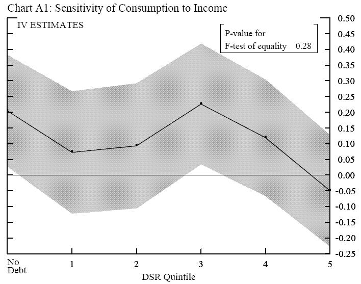
Several studies suggest that measurement error in income growth is non-classical, so the standard correction using instrumental variable (IV) estimation is invalid. In general, these studies find that measurement error in income growth violates the classical error-in-variables assumption that the error is independent of true income growth. Gervais and Klein (2006) point out that this violation can be induced by the structure of the CEX. They argue that in a model of consumption smoothing, "true" income growth is measured over the same time period as consumption growth. However, in each CEX interview, consumption includes expenditures made over the previous quarter, while income includes earnings over the previous four quarters, so measured income growth in the CEX is only an approximation of true income growth. The particular asynchrony between consumption growth and income growth can be shown to imply that under some income processes, the error in approximation may be negatively correlated with true income growth.¹¹ In addition, income validation studies of other surveys, such as the Current Population Survey (Bound and Krueger, 1991) and the Panel Study of Income Dynamics (Bound, et.al., 1994), suggest that measurement error in income growth is mean-reverting, rather than independent of the true value of income growth.

These validation studies also suggest that the bias caused by measurement error in income growth is not overwhelming. Bound and Krueger (1991) regress the "true" value of income growth on the measured value; their results imply a 23 percent downward bias in OLS estimates for men and a 15 percent downward bias for women. A similar regression in Bound, et.al. (1994) imply a 23 percent downward bias in OLS estimates. Because measurement error in income is non-classical, we will estimate equation using OLS rather than use an IV technique, but will keep in mind the effects of measurement error on our estimates.¹² We will, however, maintain the assumption that the measurement error in income is independent of the household DSR.

To help ensure that the measurement error in income is independent of the DSR, we will use expected household income in the denominator of the DSR. Expected income equals fitted income from a regression of income measured during each household's second interview on a polynomial in the age of the reference person, family size, and dummy variables for a non-white reference person, high school graduate, college graduate, and interview year.¹³ Using fitted income will also help ensure that our DSR measure is independent of the household's subsequent growth in income. To see this, suppose the DSR were calculated using debt payments and actual income collected during the second interview. If income is mean-reverting, households with temporarily low income would have both a high DSR and high income growth, creating a positive relationship between the DSR and income growth. Using expected income avoids this problem.

Smoothing variation in income

Basic result on consumption smoothing

We present first an estimate of consumption smoothing for our entire CEX sample. As shown in Table 5, the estimated parameters of equation 7 appear sensible. The estimated sensitivity of consumption to income is similar to that found by Dynarski and Gruber (1997) and Gervais and Klein (2006); a 1.0 percentage point rise in income growth leads to about a 7 basis point rise in consumption growth. Other coefficients have intuitive signs; with each additional family member, consumption grows about 7 basis points faster. Consumption grows a touch slower among households with a nonwhite household head and slightly faster among married households and households whose head earned a high school or college diploma.

Table 5: The effect of household characteristics on consumption growth

Characteristic	Parameter Estimate	Percent	StdErr
Growth in income	0.072	**	0.006
Age of the household head	0.007		0.066
agesq/100	-0.013		0.235
agecu/10000	-0.003		0.360
agefo/1000000	0.017		0.202
Change in family size	0.072	**	0.004
Non-white	-0.013	*	0.007
High school graduate	0.014	**	0.007
College Graduate	0.020	**	0.007
Married	0.016	**	0.005

**5 percent; * 10 percent

Note: Adjusted R-squared equals 0.15. Full set of month and year dummies were jointly statistically significant.

Heterogeneity in consumption smoothing, by access to credit

Next, households with different debt service ratios are allowed to smooth consumption differently. Recall our baseline specification:

$$\mbox{(7 ') }\Delta \log (C^i)=\beta _0 +\beta _1 \mbox{ }\Delta \theta ^i+\sum\limits_{q=1}^Q {\left[ {\gamma _q \left( {D_q ^i\Delta \log (Y^i)} \right)} \right]} +\xi Year^i+\eta Month^i+\varepsilon _i$$

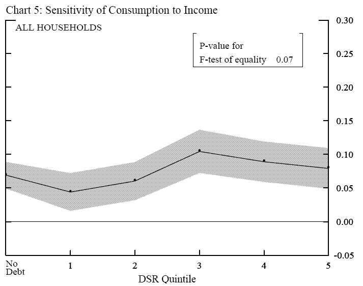
Households are placed into six groups: the first group includes households who have no debt payments, and the remaining five are the quintiles of positive debt service.

The results of this regression are shown in chart 5. The solid line plots the income coefficient for each group of households; 95 percent confidence intervals are shaded in gray. The coefficients fluctuate in a very narrow band across the DSR groups and are not higher for higher DSR households. The p-value for the F-test of whether the coefficients are equivalent, shown in the inset box, indicates that the coefficients are significantly different from one another, but this result reflects the slightly higher coefficient on quintile 3.

One reason the coefficients may lack an uptrend at the highest DSR levels is suggested in table 6. Households in the highest DSR group, the right column, do not look likely to be particularly credit constrained.¹⁴ They are slightly younger than those with lower debt service, but they have higher income on average and nearly a quarter have a college degree.

Table 6: Characteristics of CEX Sample, by DSR group

DSR Group	DRS = 0: No Debt	Lowest 20: 1	Middle 60: 2-4	Highest 20: 5
Less than highschool education (percent)	28.3	12.5	8.8	13.3
High school education (percent)	55.6	55.9	56.6	63.1
College diploma (percent)	16.1	31.6	34.6	23.6
Age (years)	44.5	44.2	43.4	42.8
Married (percent)	39.8	55.6	71.7	58.0
Black (percent)	18.4	10.8	8.5	10.7
Family size	2.6	2.7	3.1	2.8
Income (1992 $)	23,691	33,586	46,612	55,691
DSR (percent)	0.0	2.2	17.6	45.6

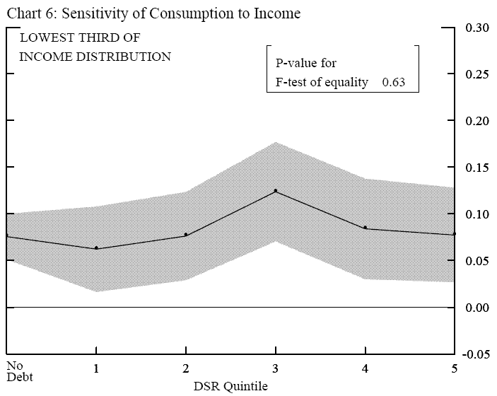
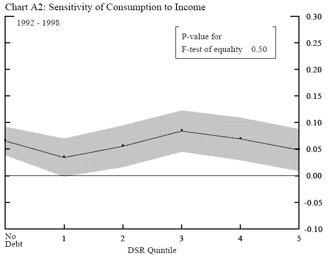
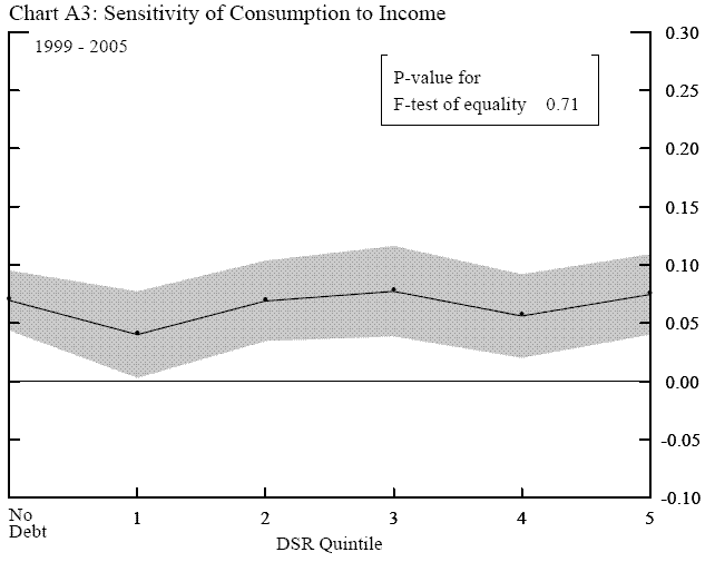
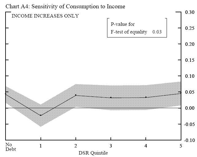
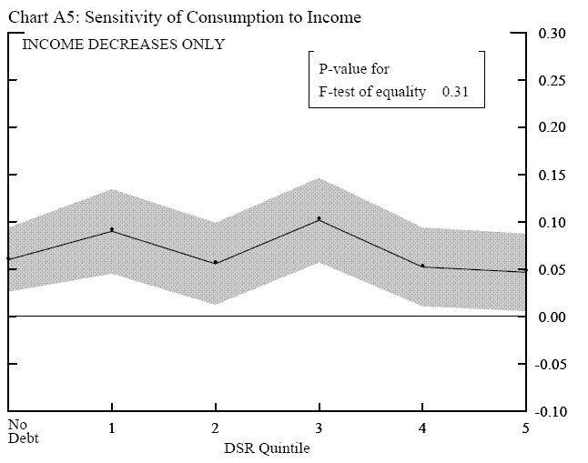
To isolate potentially more vulnerable households, we repeated our analysis, focusing on the sensitivity of consumption among households in the lowest third of the income distribution. The sensitivity of consumption for these households is plotted in chart 6. Again we find that for households with higher debt service, consumer spending is no more sensitive to income fluctuations than for households with lower debt service. These results are robust to many changes in the specification, including dividing the sample into different sub-periods and separately examining income rises and declines.¹⁵

Discussion

One possible explanation for our result is that households with high DSR are able to smooth consumption as well as other households because they have not yet exhausted their credit limits, despite having devoted a substantial share of their income to the repayment of existing debt. This in turn may reflect household's increased access to credit during the last decade and a half. However, in our CEX sample, higher debt service is associated with slower subsequent debt growth, controlling for other factors. In a regression of the change in the ratio of total debt balance to expected income on the ex ante DSR, household demographic changes, and year and month dummies, the association between the DSR and subsequent changes in the debt-to-income ratio is negative and statistically different from zero.¹⁶ The DSR coefficient implies that the debt-to-income ratio of households with a high DSR (equal to the average in DSR group 5) increases by about 5 percentage points less than the debt-to-income ratio of those with a low DSR (equal to the average in group 1). This result provides some evidence against the hypothesis that those with high debt service can borrow as much as other households.

Another explanation is that households with relatively high DSRs may have sufficient liquid assets to buffer against a change in their income. Consistent with this idea, we find that high debt service in our CEX sample is associated with high liquid assets, all else equal. In a regression of liquid assets relative to expected income on the DSR, household demographics, and year and month dummies, the association between the DSR and the asset-to-income ratio is positive and statistically different from zero.¹⁷ The DSR coefficient implies that the asset-to-income ratio of households with a high DSR is 1 percentage points higher than the asset-to-income ratio of households with a low DSR. Therefore, these results hint that high DSR households may utilize their liquid assets to smooth through income changes. However, this positive correlation is somewhat puzzling, as some households might increase their return by paying off their debt instead of holding low-return liquid assets.¹⁸

The negative correlation between DSR and debt growth suggests that a high DSR may be useful as one indicator of borrowing constraints, however the positive correlation between liquid assets and DSR likely masks this role of the DSR. To better isolate this role, we look at the effect of high DSR on consumption sensitivity among households with low liquid assets. Unfortunately, the significant number of households with invalid asset data precludes estimating equation with all five DSR groups. Instead, we placed households into just two groups, those who are in both the highest DSR group and the lowest quartile of the liquid asset distribution, which we refer to as potentially borrowing constrained households, and all other households.

Although, liquid assets have often been used in the past to identify liquidity constrained households, our CEX sample does not provide consistent evidence that the consumption of low liquid asset households is more sensitive to a change in income than the consumption of other households. For example, we find that the consumption among households in the lowest quartile of liquid assets is actually slightly less sensitive than that of other households, although this result is not robust to changes in specification.

In contrast, we find that using a household's DSR in conjunction with liquid assets consistently helps to identify households whose consumption is more sensitive to income fluctuations. The coefficient on income growth, in equation , among potentially borrowing constrained households - at 0.11 - is over 50 percent higher than among other households. Although economically meaningful, this difference is not statistically significant, with t-statistic of only 1.05, in large part because the group of high DSR, low asset households represents only about 3 percent of our sample. However, because the difference in consumption sensitivity is large and robust to changes in the specification, we feel the DSR may be useful in identifying borrowing constrained households and that more work is warranted.

Conclusion

In summary, we constructed the share of household income devoted to required payments on existing household debt (DSR) using respondents to the Consumer Expenditure Survey between 1992 and 2005. We find this household-level measure of DSR comparable to other survey data and exhibiting an upward trend that is broadly similar to a publicly-available aggregate measure of household debt service. Turning to the implications of this broad trend for household spending, we estimated the sensitivity of changes in nondurable consumption to changes in total household income across the DSR distribution. We have found that the sensitivity of changes in consumption to changes in income appears to be the same across the DSR distribution, suggesting that households with relatively high DSRs are no less able to smooth through income fluctuations than other households. This result is broadly consistent with a recent study using data from the United Kingdom suggesting that the spending of high and low debt households reacts similarly to balance sheet changes (Benito, et.al. 2007).

However, we find some evidence that, in conjunction with other information, the DSR may yet be useful to identify borrowing constrained households. In particular, the consumption of households with low liquid assets and high DSR is more sensitive to income changes than the consumption of other low liquid asset households. Although the effect of a higher DSR is not precisely estimated, it is large and robust to changes in the specification, suggesting that more work is warranted.

Admittedly, our reduced-form estimation cannot completely disentangle the factors that may increase the sensitivity of consumption to income fluctuations among households with high debt service. In addition to access to credit, these factors may include heterogeneity in time discounting. Future work must also address how these other factors may lead households to both a higher DSR and higher consumption sensitivity.

In conclusion, it seems plausible that, all else equal, higher debt obligations should make the consumption of at least some households more sensitive to cash flow but we have found only suggestive evidence that this is true. However, we should note that this result may in part reflect two limitations of the CEX data. First, the CEX data are available only through early 2005. Second, the CEX offers only limited ways to identify the most vulnerable households. While we see this research as a first step in the use of household-levelto better understand issues regarding household debt service, it suggests that the long-term uptrend in the aggregate debt service ratio is not, by itself, an indication of greater vulnerability in the household sector as a whole.

References

Bacchetta and Gerlach (1997). "Consumption and Credit Constraints: International Evidence." Journal of Monetary Economics, v. 40, n. 2, (October).

Benito, A., M. Waldron, G. Young and F. Zampolli (2007). "The Role of Household Debt and Balance Sheets in the Monetary Transmission Mechanism," Bank of England Quarterly Bulletin, 2007 Q1, pp. 70-78.

Bostic, R. (2002), "Trends in equal access to credit products," in The Impact of Public Policy on Consumer Credit. T. Durkin and M. Staten eds. Kluwer Academic Publishers. Boston.

Branch, E. R. (1994). "The Consumer Expenditure Survey: a comparative analysis." Monthly Labor Review. December. P. 47 - 55.

Bucks, B. and K. Pence (2006). "Do Homeowners Know Their House Values and Mortgage Terms?" Federal Reserve Board Finance and Economics Discussion Series 2006-3 (March).

Bureau of Labor Statistics (2006), "Consumer Expenditures and Income." BLS Handbook of Methods, Chapter 16. www.bls.gov/cex/home/htm.

Bureau of Labor Statistics (2007), "2005 Consumer Expenditure Interview Survey Public Use Microdata Documentation." http://www.bls.gov/cex/2005/cex/csxintvw.pdf.

Bound, J. and A. Krueger (1991) "The extent of measurement error in longitudinal earnings data: do two wrongs make a right?" Journal of Labor Economics, v.9, n.1, pp. 1-24.

Bound, J., C. Brown, G.J. Duncan and W.L. Rodgers (1994), "Evidence on the validity of cross-sectional and longitudinal labor market data," Journal of Labor Economics, v. 12, n.3, pp. 345-368.

Bound, J., C. Brown, and N. Mathiowetz (2001), "Measurement Error in Survey Data," in Handbook of Econometrics, vol 5. J.J. Heckman and E. Learmer, eds. Elsevier Science.

Cagan, C. (2007). "Mortgage Payment Reset: The Issue and the Impact." Research Study, First American CoreLogic. www.firstam.com

Coulibaly B., and G. Li (2006). "Do Homeowners Increase Consumption after the Last Mortgage Payment? An Alternative Test of the Permanent Income Hypothesis." The Review of Economics and Statistics. 88(1) p. 10-19.

Debelle, Guy (2004). "Macroeconomic Implications of Rising Household Debt." BIS Working Papers, n. 153.

Dynan, K. and D. Kohn (2007). "The Rise in U.S. Household Indebtedness: Causes and Consequences." Federal Reserve Board Finance and Economics Discussion Series 2007-37.

Dynan, K., K. Johnson and K. Pence (2003). "Recent Changes to a Measure of U.S. Household Debt Service." Federal Reserve Bulletin, September.

Dynarski, S. and J. Gruber (1997). "Can Families Smooth Variable Earnings?" Brookings Papers on Economic Activity, 1997(1), p. 229-303.

Gervais, M. and P. Klein (2006), "Measuring Consumption Smoothing in CEX Data," mimeo.

Gieseman, R. (1987). "The Consumer Expenditure Survey: quality control by comparative analysis." Monthly Labor Review, March. P. 8-14.

Gross, D. and N. Souleles (2002). "Do Liquidity Constraints and Interest Rates Matter for Consumer Behavior? Evidence from Credit Card Data." Quarterly Journal of Economics. 117 (1) February.

Jappelli, T. (1990). "Who is Credit Constrained in the U.S.?" Quarterly Journal of Economics. 105(1), p 219-34.

Johnson, Kathleen W. (2007), "The Transactions Demand for Credit Cards." The B.E. Journal of Economic Analysis & Policy, 7(1) http://www.bepress.com/bejeap/vol7/iss1/art16

Johnson, Kathleen W. (2005), "Recent Developments in the Credit Card Market and the Financial Obligations Ratio." Federal Reserve Bulletin, (Autumn) p. 473-486.

Kennickell, A. and R.L. Woodburn (1997), "Consistent Weight Design for the 1989, 1992, and 1995 SCFs, and the Distribution of Wealth." http://www.federalreserve.gov/pubs/oss/oss2/papers/wgt95.pdf

Ludvigson, S. (1999). "Consumption and Credit: A Model of Time-Varying Liquidity Constraints." Review of Economics and Statistics, v. 81, n. 3 (August) p. 434-47.

Lusardi, A. (1996) "Permanent Income, Current Income and Consumption: Evidence from Two Panel Data Sets," Journal of Business and Economic Statistics, v. 14, n.1 (January) pp. 81-90.

Maki (2002). "The Growth of Consumer Credit and the Household Debt Service Burden" in The Impact of Public Policy on Consumer Credit. T. Durkin and M. Staten eds. Kluwer Academic Publishers. Boston.

McCarthy (1997). "Debt, Delinquencies and Consumer Spending" Current Issues in Economics and Finance, Federal Reserve Bank of New York (February).

Mishkin (1976). "Illiquidity, Consumer Durable Expenditures, and Monetary Policy." American Economic Review, v. 66, n. 4, (September).

Stephens, M. (2005). "The Consumption Response to Predictable Changes in Discretionary Income: Evidence from the Repayment of Vehicle Loans." Working paper. http://www.andrew.cmu.edu/user/melvins/

Data Appendix - Variable definitions

Consumer Unit (CU) - a consumer unit comprises either: (1) all members of a particular household who are related by blood, marriage, adoption or other legal arrangements; (2) a person living alone or sharing a household with others or living as a roomer in a private home or lodging house or in a permanent living quarters in a hotel or motel, but who is financial independent; or (3) two or more persons living together who use their income to make joint expenditures. Financial independence is determined by the three major expense categories: housing, food and other living expenses. To be considered financially independent, at least two of the three major expense categories have to be provided entirely or in part by the respondent.

Reference person - The first member mentioned by the respondent when asked to "Start with the name of the person or one of the persons who owns or rents the home." It is with respect to this person that the relationship of other CU members is determined.

Consumption -Calculated from data reported in the Monthly Expenditures (MTAB) file. In the MTAB file, expenditures reported by a CU are identified by UCC and month in which the expenditure occurred.

Consumption is assumed to equal expenditures on nondurable goods as defined in Lusardi (1996). Nondurable goods expenditure includes those on food, alcoholic beverages, public transportation, utilities, household operations, gasoline, personal care, tobacco, apparel, health care products, reading materials, educational expenses and miscellaneous from the following UCC codes:

190904, 790220, 790230, 190901, 190902, 190903, 790410, 790430, 200900, 790310, 790320, 790420, 530110-530902, 250111-270214, 270411-270904, 330511, 340210-340530, 340620-340901, 340906-340908, 340903, 670310, 690113, 470111-470212, 640130-650900, 630110-630210, 680110-680902, 620112, 710110, 790600, 880210, 360110-430120, 440110-440900, 540000-480902, 590110-590230, 660110-660210, 660900-670210, 670901-670902.

Income before taxes - Reported on the Consumer Unit Characteristics and Income (FMLY) file. The combined income earned by all CU members 14 years old or over during the 12 months preceding the interview. The components of income are: Wage and salary income before deductions, income or loss from non-farm business, income or loss from farm, Social Security income and Supplemental Security Income, unemployment compensation, worker's compensation and veterans' benefits, public assistance, interest on savings accounts and bonds, income from dividends royalties and trusts, pensions and annuities, income from boarders or rental units, child support, alimony, scholarships, etc., food stamps.

Debt payments - Payments on mortgage, auto loans and home equity loans from the MTAB file plus payments on credit card loans. In the MTAB files, debt payments include principal and interest expenditures associated with the UCC codes for each type of secured debt. For example, auto loans debt payments include UCC codes:

850100 Reduction of principal on vehicle loan

870103 Finance charges on loans for new cars, trucks, or vans

870203 Finance charges on loans for used cars, trucks, or vans

870803 Interest, other vehicle, financed

Payments on credit card loans equal 2 percent of the outstanding balance reported in the FMLY file.

Debt service ratio - The ratio of debt payments to expected income. Expected income equals fitted income from a regression of the average income from each household's second and fifth interview on the age of the reference person, age squared, age cubed, and dummy variables for non-white reference person, high school graduates, and college graduates.

Age - Age of the CU reference person.

Change in family size - Change in the number of members in the CU.

Non-white - Race of the reference person Black, Native American, Asian, Pacific Islander or Multi-race.

High school graduate - Reference person earned a high school diploma and may have some college education but did not earn a degree.

College graduate - Reference person earned an Associate's, Bachelor's, Master's, Professional or Doctorate degree.

Married - Marital status of reference person is married.

Sample selection procedure -

• keep only households with uninterrupted debt payments, i.e. the households have not stopped paying for one or two quarters then started paying again
• delete households living in student housing facilities
• delete households with non-positive income
• trim off the top and bottom 1 percent of log income and expenditure growth
• head of household older than 25, but younger than 64 (inclusive)
• DSR lower than 2
• valid data for family size , race, education and marital status

The final sample includes 28,791 households.

Appendix Charts and Tables

Table A1 Debt Balance and Payments by year and survey

Year / Survey	1992: SCF	1992: CEX	1992: SCF / CEX	1995: SCF	1995: CEX	1995: SCF / CEX	1998: SCF	1998: CEX	1998: SCF / CEX	2001: SCF	2001: CEX	2001: SCF / CEX	2004: SCF	2004: CEX	2004: SCF / CEX
Mean Total Payments	5572	5912	0.942	6137	6523	0.941	7618	7783	0.979	8616	8912	0.967	10131	10366	0.977
Mean Total Debt Balance	29158	27554	1.058	33518	34392	0.975	42701	38106	1.121	50342	46889	1.074	74045	66092	1.120
Mean Mortgage Payments	3485	3749	0.930	3788	4203	0.901	4657	4761	0.978	5397	5651	0.955	6240	6918	0.902
Mean Mortgage Balance	24959	22796	1.095	28637	28993	0.988	36153	30880	1.171	42673	39192	1.089	62600	56931	1.100
Ratio of Mortgage 0	38.22%	39.45%		39.39%	42.07%		41.16%	41.58%		42.28%	44.26%		44.91%	48.30%
Mean Other Real Estate Loans Payments	747	712	1.049	711	506	1.405	1015	701	1.448	966	763	1.266	747	745	1.003
Mean Other Real Estate Loans Balance	1170	1710	0.684	863	1194	0.723	1360	1975	0.689	1904	2149	0.886	4270	2360	1.809
Ratio of Other Real Estate Loans 0	13.19%	10.86%		11.41%	9.66%		14.13%	12.64%		12.26%	12.64%		14.93%	11.71%
Mean Vehicle Loan Payments	1036	1155	0.897	1214	1371	0.885	1401	1761	0.796	1700	1935	0.879	1895	2046	0.926
Mean Vehicle Loan Balance	2018	2055	0.982	2605	2728	0.955	3371	3382	0.997	3927	3669	1.070	4804	4612	1.042
Ratio of Vehicle Loan 0	29.47%	34.76%		31.56%	35.75%		31.24%	40.32%		34.81%	38.47%		35.60%	40.07%
Mean Credit Card Payments	303	298	1.017	424	443	0.957	545	561	0.971	551	564	0.977	711	657	1.082
Mean Credit Card Balance	1011	994	1.017	1413	1476	0.957	1817	1869	0.972	1837	1879	0.978	2372	2190	1.083
Ratio of Credit Card 0	43.70%	45.26%		47.26%	48.20%		44.10%	49.72%		44.38%	44.91%		46.17%	42.12%

Table A2: Regression of Log Income for DSR Calculation.

Variable	Estimate	Percent	StdErr
Intercept	7.722	**	0.215
Age	0.037	**	0.019
Age square	0.120	**	0.056
Age cubed	-0.389	**	0.072
Age fourthed	0.248	**	0.033
High school	0.345	**	0.011
Some college	0.505	**	0.011
College	0.846	**	0.011
White	0.190	**	0.010
Married	0.536	**	0.008
Family size	0.062	**	0.003

**5 percent; * 10 percent

Note: Full set of year dummies were jointly statistically significant.

Instrumental Variable Estimates

Table A3: The effect of household characteristics on consumption growth - IV estimates

Characteristic	Parameter Estimate	Percent	Standard Error
Growth in income	0.110	**	0.044
Age of the household head	-0.031		0.100
agesq/100	0.094		0.358
agecu/10000	-0.132		0.557
agefo/1000000	0.072		0.317
Change in family size	0.071	**	0.006
Non-white	-0.020	*	0.011
High school graduate	0.021	*	0.011
College Graduate	0.019		0.012
Married	0.016	**	0.007

Robustness of main finding

Footnotes

1. Kathleen Johnson, Mail Stop #93, Board of Governors of the Federal Reserve System, Washington DC 20551; e-mail: [email protected]; phone (202) 452-3644. Geng Li, Mail Stop #93, Board of Governors of the Federal Reserve System, Washington DC 20551; e-mail: [email protected] ; phone (202) 452-2995. The opinions, analysis, and conclusions of this paper are solely the authors' and do not necessarily reflect those of the Board of Governors of the Federal Reserve System or its staff. The authors would like to thank Orazio Attanasio, Chris Carroll, Karen Dynan, Fumiko Hayashi, and seminar participants at the Federal Reserve Board, the 2007 Midwest Macro Meetings, the 2007 Federal Reserve System Applied Microeconomics Conference, the 2007 NBER Summer Institute, and the FDIC Center for Financial Research for helpful comments on an earlier draft. All remaining errors are our own. Return to Text

2. For a given level of debt, a fall in the interest rate will also reduce the debt payment, but this effect is small relative to the effect of a rise in debt balances on debt payments. Return to Text

3. p. 21. Return to Text

4. We do not use household's reported payments on credit card debt in part because respondents are asked to include only interest payments. Thus, debt service on credit card debt is calculated using the concept employed by the Federal Reserve System in their aggregate DSR measure. That is, households are assumed subject to a minimum credit card payment of 2 percent of their outstanding credit card balance. Return to Text

5. CEX respondents report payments for each quarter, whereas SCF respondents report average monthly debt payments so all payments were converted to an annual rate. In addition, we compared the CEX respondents who were first interviewed in the year corresponding to a SCF wave. Because CEX respondents were interviewed for several successive quarters, this implies that some of the CEX debt payment data may have been collected in the following year. Underlying data are shown in appendix table A1. Return to Text

6. Each of the means is weighted using sampling weights and thus represents the average debt payment for all households in the United States. For a full discussion of the sampling weights in each of the surveys, see Kennickell and Woodburn (1997) and Bureau of Labor Statistics (2007). Return to Text

7. Because credit card debt service is a constant share of credit card debt outstanding, the congruence between required debt payments in the two surveys reflects that of credit card debt outstanding. Return to Text

8. We smoothed the time trend by regressing the year effects on time and plotting the resulting regression line. Return to Text

9. See the data appendix for a full description of each of the variables used in the following analysis. Return to Text

10. The proportions and means presented in this section are intended to paint a picture of the sample used for estimation, and as such are not weighted by the CEX population weights. Return to Text

11. Whether this asynchrony is an issue depends on households' income process. If income growth is constant over time (for example , the CEX approximation will equal true income growth and measurement error equals zero. However, if income growth is time-dependent (for example: the measurement error will be negatively correlated with true income growth. Return to Text

12. In an earlier version of this paper, we instrumented income with earned income, which was constructed from the number of hours worked per pay period and the wages earned during the pay period. These results are presented in Appendix table 3 and chart 1. Return to Text

13. The results of this regression are shown in Appendix table 2. Return to Text

14. Indeed, households with no debt look the most credit constrained. The demographic and financial characteristics of this group resemble those of households with a high probability of being turned down for credit (Jappelli, 1990). Eighteen percent of households with no debt payments have a non-white household head, compared to about nine percent of households with positive debt payments. The head of a household with no debt payments is more than twice as likely to be without a high school diploma, and is significantly less likely to be married as the head of a household with positive debt payments. Finally, households with no debt payments earn significantly less income, on average, than households with positive debt payments. Return to Text

15. The results of these regressions are presented in Appendix charts 2-5. Return to Text

16. We use the same set of control variables as equation . The DSR coefficient in this regression equals -0.12 with a t-statistic of -6.31. Return to Text

17. The controls in this regression are similar to those in , but focus on levels and not changes in demographics. The DSR coefficient in this regression is 0.04 with a t-statistic of 3.73. Return to Text

18. A similar puzzle was also pointed out by Gross and Souleles (2002). Return to Text

This version is optimized for use by screen readers. Descriptions for all mathematical expressions are provided in LaTex format. A printable pdf version is available. Return to Text

Home | Economic Research and Data | Accessibility | Contact us
Last update: October 22, 2007