
Productivity, Aggregate Demand and Unemployment Fluctuations*
Keywords: Unemployment fluctuations, labor productivity, search and matching model, New-Keynesian model
Abstract:
JEL classifications: J64, E32, E37, E52
1. Introduction
What drives unemployment fluctuations at business cycle frequencies? Since the seminal work of Mortensen-Pissarides (1994), a vast literature, including the influential work from Shimer (2005a), has focused on labor productivity to explain movements in unemployment.1 In a Mortensen-Pissarides (MP) search and matching model, an increase in productivity raises the surplus of a match between a firm and a worker, leads firms to post more job vacancies and pulls down the unemployment rate. Shifts in labor demand are caused by changes in productivity, and productivity is seen as the central driving force of unemployment fluctuations.
Given the major role played by productivity, there is surprisingly little empirical evidence on the impact of productivity changes on unemployment. In fact, this paper uncovers new empirical findings that are inconsistent with the standard MP prediction that an increase in productivity leads to lower unemployment. I argue that the inconsistency arises because the MP model does not allow output to be demand determined in the short run, and I present a search model with nominal rigidities that can rationalize the empirical findings. In addition, I show that the interaction of hiring frictions and nominal frictions can generate a new propagation mechanism absent in standard New-Keynesian models.
The first contribution of this paper is empirical. It provides a thorough study of the relationship between unemployment fluctuations and labor productivity (measured as real output per hour) in the US and highlights new empirical facts that posit a challenge to the standard MP model. I find
that ![]() , the contemporaneous correlation between labor productivity and unemployment switched sign in the mid 80s; from negative it became positive. Furthermore, I find that a positive
technology shock, identified as in Gali (1999) as the only disturbance with a permanent impact on labor productivity, increases unemployment temporarily, whereas a positive non-technology shock (temporarily) increases productivity and decreases unemployment.
, the contemporaneous correlation between labor productivity and unemployment switched sign in the mid 80s; from negative it became positive. Furthermore, I find that a positive
technology shock, identified as in Gali (1999) as the only disturbance with a permanent impact on labor productivity, increases unemployment temporarily, whereas a positive non-technology shock (temporarily) increases productivity and decreases unemployment.
The standard search model of unemployment is confronted with two problems. First, it predicts that an increase in productivity leads to lower unemployment and implies a negative value for ![]() Second, with only one mechanism through which productivity affects the labor market, it cannot generate two different impulse responses or explain large changes in
Second, with only one mechanism through which productivity affects the labor market, it cannot generate two different impulse responses or explain large changes in ![]() .
.
The second contribution of this paper is theoretical. I develop a tractable search and matching model with nominal rigidities in which hiring firms are demand constrained in a New-Keynesian fashion. I also make a distinction between the extensive (number of workers) and the intensive (hours and
effort) labor margins. In this framework, unemployment fluctuations are the product of two disturbances: technology shocks and monetary policy (or aggregate demand) shocks. Positive technology shocks temporarily raise unemployment because with sticky prices, aggregate demand does not adjust
immediately to the new productivity level, and firms use less labor. The correlation between unemployment and productivity, ![]() , is positive. In contrast, positive aggregate demand
disturbances decrease unemployment and increase productivity temporarily, because firms increase labor effort to satisfy demand in the short run. As a result,
, is positive. In contrast, positive aggregate demand
disturbances decrease unemployment and increase productivity temporarily, because firms increase labor effort to satisfy demand in the short run. As a result, ![]() is negative. In this model,
movements in
is negative. In this model,
movements in ![]() reflect changes in the relative importance (or volatility) of technology and aggregate demand shocks.
reflect changes in the relative importance (or volatility) of technology and aggregate demand shocks.
The volatility of the non-technology shocks identified with long run restrictions displays a large drop in the early 80s. By interpreting non-technology shocks as aggregate demand shocks in the model, this can explain why ![]() increased. Model simulations suggest that changes in shock volatilities can account for about 40 percent of the increase in
increased. Model simulations suggest that changes in shock volatilities can account for about 40 percent of the increase in ![]() . Evidently some other
force must be at work. New evidence suggests that a structural change took place in the early 80s and that productivity became less procyclical, i.e. the endogenous component of productivity due to variable capacity utilization of inputs decreased. With a less endogenous response of productivity,
the negative impact that aggregate demand shocks have on
. Evidently some other
force must be at work. New evidence suggests that a structural change took place in the early 80s and that productivity became less procyclical, i.e. the endogenous component of productivity due to variable capacity utilization of inputs decreased. With a less endogenous response of productivity,
the negative impact that aggregate demand shocks have on ![]() is diminished. This can also explain why
is diminished. This can also explain why ![]() increased. I simulate the impact of the simultaneous structural change and drop in the volatility of aggregate demand shocks, and I find that these two events can quantitatively explain the sign switch of
increased. I simulate the impact of the simultaneous structural change and drop in the volatility of aggregate demand shocks, and I find that these two events can quantitatively explain the sign switch of ![]() in the mid 80s.
in the mid 80s.
Moreover, the combination of two major macroeconomic frameworks, the New-Keynesian model and the MP model, has interesting properties that extend beyond the explanation of unemployment fluctuations. By explicitly considering the interaction between hiring frictions and nominal frictions and by allowing labor to adjust along the extensive and intensive margin, the model highlights a new propagation mechanism that originates in the trade-off existing between the two labor inputs: the extensive margin can be less expensive than the intensive one but it is also less flexible because of hiring frictions. Once the firm has posted its price, demand (and hence revenue) is given, and the contribution of an additional worker is not its marginal product. Instead, it is the reduction of the wage bill through substitution of an expensive input (the intensive margin) for a cheaper one (the extensive margin), and the firm chooses the combination of labor inputs that minimizes the cost of supplying the required amount of output. In this setup, I show that the volatility of unemployment and the persistence of inflation increase with the magnitude of the trade-off.
The seminal contributions of Galí (1999) and Basu, Fernald and Kimball (1999) spawned an important empirical literature on the negative effect of technology shocks on total hours worked, but the focus has mostly been on hours and not employment or unemployment. Galí (1999) offered
a New-Keynesian explanation, and the present model invokes a similar mechanism to account for an increase in unemployment following a technology shock. A growing literature introduces search models of unemployment into New-Keynesian frameworks but to my knowledge, this paper is the first to propose
a model emphasizing the interaction between hiring frictions and nominal frictions and capable of rationalizing large movements in ![]() . Models in the spirit of Trigari (2004) or Walsh (2004)
introduce a separation between firms facing price stickiness (the retail sector) and firms evolving in a MP labor market without nominal rigidities (the wholesale sector).2 While the separation simplifies greatly the analysis, this paper shows that it is possible to model the interaction of both frictions without compromising tractability. In Krause and Lubik (2007), hiring firms are demand constrained, but without intensive margin, the
model displays a different propagation mechanism and cannot generate endogenous productivity movements. Finally, Blanchard and Galí (2008) incorporate both hiring and nominal frictions in a very elegant framework but without modeling the intensive margin and with a focus on optimal monetary
policy.
. Models in the spirit of Trigari (2004) or Walsh (2004)
introduce a separation between firms facing price stickiness (the retail sector) and firms evolving in a MP labor market without nominal rigidities (the wholesale sector).2 While the separation simplifies greatly the analysis, this paper shows that it is possible to model the interaction of both frictions without compromising tractability. In Krause and Lubik (2007), hiring firms are demand constrained, but without intensive margin, the
model displays a different propagation mechanism and cannot generate endogenous productivity movements. Finally, Blanchard and Galí (2008) incorporate both hiring and nominal frictions in a very elegant framework but without modeling the intensive margin and with a focus on optimal monetary
policy.
The remainder of the paper is organized as follows: Section ![]() studies the relationship between labor productivity and unemployment; Sections
studies the relationship between labor productivity and unemployment; Sections ![]() and
and ![]() describe the model and its properties; Section
describe the model and its properties; Section ![]() explores whether the model can quantitatively account for the empirical impulse responses to shocks and the change in the sign of
explores whether the model can quantitatively account for the empirical impulse responses to shocks and the change in the sign of ![]() ; Section
; Section ![]() discusses an alternative interpretation of the sign switch for
discusses an alternative interpretation of the sign switch for ![]() ; and Section
; and Section ![]() offers some concluding remarks.
offers some concluding remarks.
2.1 The  puzzle
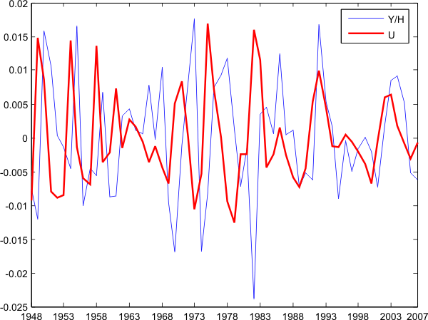
Figure ![]() shows the detrended series for US unemployment and labor productivity (i.e. output per hour) over 1948-2007.3 Until 1985, the two series seem negatively correlated with unemployment lagging labor productivity. After 1985, however, the correlation becomes positive. This is especially true for 1992 when both unemployment and labor
productivity increase sharply but it is apparent throughout the post-1985 period. The magnitude of this sign flip is large: looking at Table
shows the detrended series for US unemployment and labor productivity (i.e. output per hour) over 1948-2007.3 Until 1985, the two series seem negatively correlated with unemployment lagging labor productivity. After 1985, however, the correlation becomes positive. This is especially true for 1992 when both unemployment and labor
productivity increase sharply but it is apparent throughout the post-1985 period. The magnitude of this sign flip is large: looking at Table ![]() ,
, ![]() goes from
goes from ![]() over 1948-1984 to
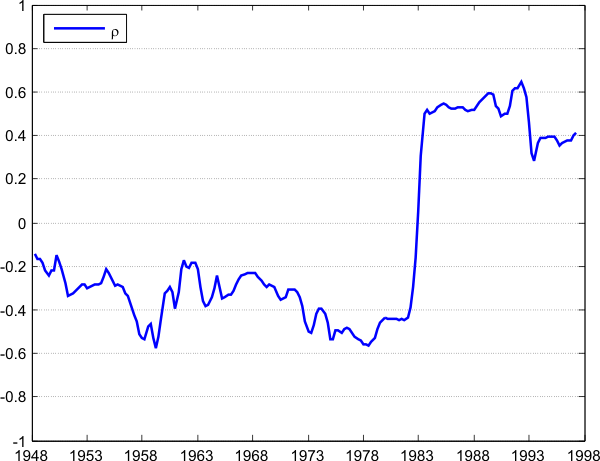
over 1948-1984 to ![]() over 1985-2007, and both estimates are significant at the 5%-level.4 To see more sharply this change in the correlation, Figure
over 1985-2007, and both estimates are significant at the 5%-level.4 To see more sharply this change in the correlation, Figure ![]() plots
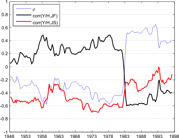
plots ![]() , the 10-year rolling contemporaneous correlation between unemployment and labor
productivity. In about a year's time, the rolling correlation switches swiftly from negative to positive values. But
, the 10-year rolling contemporaneous correlation between unemployment and labor
productivity. In about a year's time, the rolling correlation switches swiftly from negative to positive values. But ![]() also displays large fluctuations throughout the whole period, and
before 1984,
also displays large fluctuations throughout the whole period, and
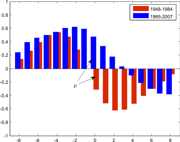
before 1984, ![]() deviates sometimes by 50% from its 1948-1984 mean. The unemployment-productivity cross-correlogram before and after 1985 gives the same conclusion. As we can see on
Figure
deviates sometimes by 50% from its 1948-1984 mean. The unemployment-productivity cross-correlogram before and after 1985 gives the same conclusion. As we can see on
Figure ![]() , the two cross-correlograms look dramatically different. Notably, the correlation between unemployment and labor productivity lagged two quarters is positive after 1985 but corresponds
to the peak negative correlation before 1985.
, the two cross-correlograms look dramatically different. Notably, the correlation between unemployment and labor productivity lagged two quarters is positive after 1985 but corresponds
to the peak negative correlation before 1985.
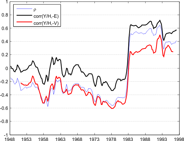
As a robustness check, I verify that the swift jump of ![]() is not the result of a change in the definition of unemployment or the labor force: in Figure
is not the result of a change in the definition of unemployment or the labor force: in Figure ![]() , I plot the 10-year rolling correlation between employment (in millions) and output per hour and the 10-year rolling correlation between vacancies and output per hour.5 Both display a large jump similar to
, I plot the 10-year rolling correlation between employment (in millions) and output per hour and the 10-year rolling correlation between vacancies and output per hour.5 Both display a large jump similar to ![]() . Table
. Table ![]() confirms this result as the correlation between productivity and vacancies went from
confirms this result as the correlation between productivity and vacancies went from ![]() over 1951-1984 to
over 1951-1984 to ![]() over 1985-2005.
over 1985-2005.
Finally, in Figure ![]() , I consider unemployment inflows and outflows, and I plot the 10-year rolling correlation between the job finding probability and output per hour and the 10-year rolling
correlation between the employment exit probability and output per hour.6 While the correlation with the job finding probability behaves similarly to
, I consider unemployment inflows and outflows, and I plot the 10-year rolling correlation between the job finding probability and output per hour and the 10-year rolling
correlation between the employment exit probability and output per hour.6 While the correlation with the job finding probability behaves similarly to
![]() , the correlation with the employment exit probability remains roughly constant and negative, displaying only a small jump in the mid-80s. This suggests that an explanation of the behavior
of
, the correlation with the employment exit probability remains roughly constant and negative, displaying only a small jump in the mid-80s. This suggests that an explanation of the behavior
of ![]() lies with inflows to unemployment and not outflows.
lies with inflows to unemployment and not outflows.
2.2 The impact of technology shocks on unemployment
There is little empirical evidence on the impact of productivity movements on cyclical unemployment. Galí (1999) and Basu, Fernald and Kimball (1999) spawned an important literature on the negative effect of technology shocks on total hours worked and its implication for business cycle models. However, the issue has little been studied in the context of models of unemployment.7
Galí (1999), following the seminal work by Blanchard and Quah (1989), impose long-run restrictions in a structural VAR model to identify technological disturbances. Technology shocks are identified as the only shocks with a permanent impact on productivity. Using a similar framework, I study the response of unemployment (instead of hours) to a technology shock. Specifically, I am interested in estimating the system
where
I use quarterly data taken from the U.S. Bureau of Labor Statistics (BLS) covering the period 1948:Q1 to 2007:Q4. Labor productivity ![]() is measured as real average output per hour in the
non-farm business sector, and unemployment
is measured as real average output per hour in the
non-farm business sector, and unemployment ![]() is the quarterly average of the monthly unemployment rate series constructed by the BLS from the Current Population Survey. Following Fernald
(2007), I allow for two breaks in
is the quarterly average of the monthly unemployment rate series constructed by the BLS from the Current Population Survey. Following Fernald
(2007), I allow for two breaks in
![]() , 1973:Q1 and 1997:Q1, and I filter the unemployment series with a cubic trend. Fernald (2007) showed that the presence of a low-frequency correlation between labor productivity
growth and unemployment, while unrelated to cyclical phenomena, could significantly distort the estimates of short run responses obtained with long run restrictions.8
, 1973:Q1 and 1997:Q1, and I filter the unemployment series with a cubic trend. Fernald (2007) showed that the presence of a low-frequency correlation between labor productivity
growth and unemployment, while unrelated to cyclical phenomena, could significantly distort the estimates of short run responses obtained with long run restrictions.8
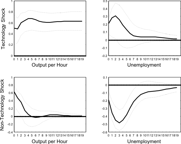
The first row of Figure ![]() displays the impulse response functions of productivity and unemployment following a technology shock. Labor productivity undershoots its new long run level by
around 20% and plateaus after about one and a half years. After an initial jump, unemployment displays a hump-shaped positive response that peaks quite rapidly, in about 2 quarters. Quantitatively, a 0.5% rise in productivity is associated with a 0.2 percentage point increase in unemployment. The second row of Figure
displays the impulse response functions of productivity and unemployment following a technology shock. Labor productivity undershoots its new long run level by
around 20% and plateaus after about one and a half years. After an initial jump, unemployment displays a hump-shaped positive response that peaks quite rapidly, in about 2 quarters. Quantitatively, a 0.5% rise in productivity is associated with a 0.2 percentage point increase in unemployment. The second row of Figure ![]() shows the dynamic effects of a non-technology shock. On impact, productivity jumps by 0.6% and reverts to its long run value
in one year. Unemployment decreases, reaches a trough after one year, and reverts slowly to its long run value. Quantitatively, a 0.6% increase in productivity is correlated with a 0.2 percentage point drop in unemployment.
shows the dynamic effects of a non-technology shock. On impact, productivity jumps by 0.6% and reverts to its long run value
in one year. Unemployment decreases, reaches a trough after one year, and reverts slowly to its long run value. Quantitatively, a 0.6% increase in productivity is correlated with a 0.2 percentage point drop in unemployment.
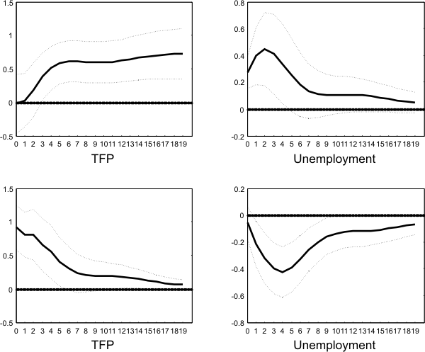
As a robustness check, I reproduce this exercise using the TFP series from Beaudry and Portier (2006) instead of output per hour in (1).9
Figure ![]() shows the impulse response functions to technology and non-technology shocks. Encouragingly, the impulse responses look very similar to the ones using output per hour, and technology
shocks increase unemployment temporarily.
shows the impulse response functions to technology and non-technology shocks. Encouragingly, the impulse responses look very similar to the ones using output per hour, and technology
shocks increase unemployment temporarily.
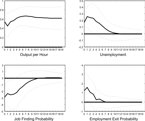
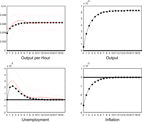
Finally, I estimate a higher dimensional (4 variable) VAR with the (logged) job finding probability and the (logged) employment exit probability as additional variables.10 Figure ![]() plots the impulse responses to a positive technology shock. The responses of unemployment and output per hour are similar to the ones obtained from a
bivariate VAR. The job finding probability declines significantly on impact and after two quarters displays a similar behavior to that of unemployment. The employment exit probability increases on impact before reverting quickly to its long run value. However, the initial response is only
marginally significant.
plots the impulse responses to a positive technology shock. The responses of unemployment and output per hour are similar to the ones obtained from a
bivariate VAR. The job finding probability declines significantly on impact and after two quarters displays a similar behavior to that of unemployment. The employment exit probability increases on impact before reverting quickly to its long run value. However, the initial response is only
marginally significant.
2.3 Confronting the MP model with the data
These results confront the standard search model with productivity shocks used in Mortensen-Pissarides (1994), Shimer (2005a) or Hall (2005) with two problems. First, it predicts a negative value for ![]() , as an increase in productivity raises the surplus of a match, leads firms to post more vacancies and pulls down the unemployment rate. However,
, as an increase in productivity raises the surplus of a match, leads firms to post more vacancies and pulls down the unemployment rate. However, ![]() is positive since the
mid 80s, and I find that a positive technology shock increases unemployment in the short run. Second, the standard MP model cannot account for changes in the sign of
is positive since the
mid 80s, and I find that a positive technology shock increases unemployment in the short run. Second, the standard MP model cannot account for changes in the sign of ![]() because it embeds only
one mechanism through which productivity affects the labor market.
because it embeds only
one mechanism through which productivity affects the labor market.
I now argue that the interaction of technology and non-technology shocks is key to understand the behavior of ![]() .
.
2.3.1 A change in the volatility of shocks
Since technology and non-technology shocks generate opposite comovements of unemployment and productivity, ![]() will depend on their relative strength. If the average "size" of one type of
shock increased relative to the other, the resulting correlation could theoretically switch between positive and negative values. For example, smaller non-technology shocks or larger technology shocks would increase
will depend on their relative strength. If the average "size" of one type of
shock increased relative to the other, the resulting correlation could theoretically switch between positive and negative values. For example, smaller non-technology shocks or larger technology shocks would increase ![]() . Figure
. Figure ![]() shows the 5-year rolling standard deviations of technology and non-technology shocks previously identified. Although the variances of both shocks
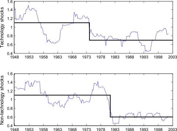
display a downward trend, it is more pronounced for non-technology shocks, with a large drop in the mid 80s.11 The standard deviation of non-technology
shocks decreased by more than 70% while the standard deviation of technology shocks was roughly constant in the mid 80s. Was the sign switch of
shows the 5-year rolling standard deviations of technology and non-technology shocks previously identified. Although the variances of both shocks
display a downward trend, it is more pronounced for non-technology shocks, with a large drop in the mid 80s.11 The standard deviation of non-technology
shocks decreased by more than 70% while the standard deviation of technology shocks was roughly constant in the mid 80s. Was the sign switch of ![]() caused by a large decrease in the volatility
of all shocks except for technological shocks? In Figure
caused by a large decrease in the volatility
of all shocks except for technological shocks? In Figure ![]() , I plot simultaneously
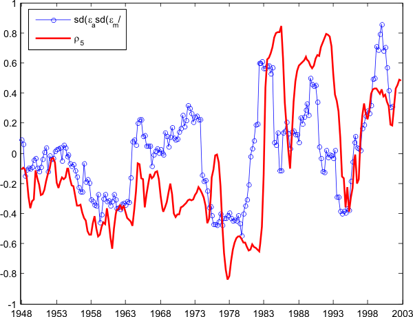
, I plot simultaneously ![]() , the 5-year rolling correlation between unemployment and labor productivity, and the ratio of the 5-year rolling standard deviation of technology shocks to the 5-year rolling standard deviation of non-technology shocks. The result is striking: the two series look very similar
despite different construction methods. Moreover,
, the 5-year rolling correlation between unemployment and labor productivity, and the ratio of the 5-year rolling standard deviation of technology shocks to the 5-year rolling standard deviation of non-technology shocks. The result is striking: the two series look very similar
despite different construction methods. Moreover, ![]() lags the shock series by about a year, suggesting a causal role for volatility fluctuations and an explanation for the sign flip of
lags the shock series by about a year, suggesting a causal role for volatility fluctuations and an explanation for the sign flip of
![]() .
.
2.3.2 Structural changes
The discussion so far has ignored structural changes as a potential explanation for rapid movements in ![]() . In fact, significant changes occurred in the early- to mid 80s: a change in the
conduct of monetary policy, a change in inventory management and a change in the regulatory environment.12 Moreover these changes could bias impulse
response functions identified over the whole post-WWII period. Analyzing the response of total hours worked to technology shocks, Galí, López-Salido and Vallés (2003) and Fisher (2006) report very different impulse response functions after splitting their data over two
sub-periods before and after the early 80s.
. In fact, significant changes occurred in the early- to mid 80s: a change in the
conduct of monetary policy, a change in inventory management and a change in the regulatory environment.12 Moreover these changes could bias impulse
response functions identified over the whole post-WWII period. Analyzing the response of total hours worked to technology shocks, Galí, López-Salido and Vallés (2003) and Fisher (2006) report very different impulse response functions after splitting their data over two
sub-periods before and after the early 80s.
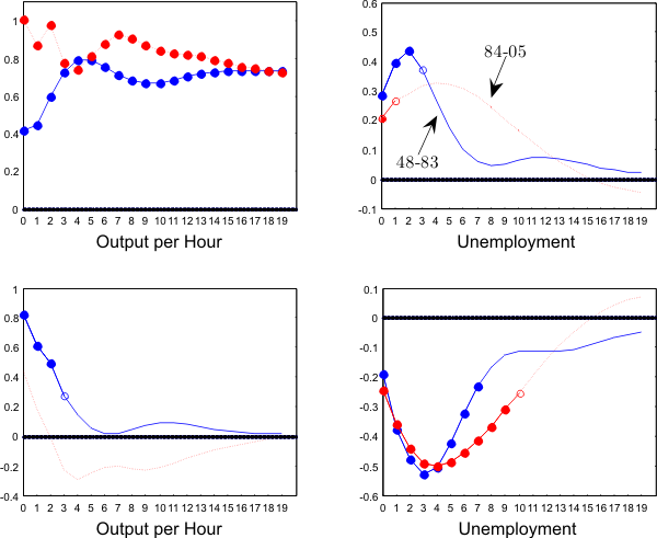
To allow for a structural change, I also split the sample in two sub-periods, 1948-1983 and 1984-2005, and Figure ![]() shows the impulse responses obtained for each period. The responses
differ in two points: (a) technology shocks have a smaller impact on unemployment after 1984, and (b) non-technology shocks have a smaller impact on labor productivity after 1984.
shows the impulse responses obtained for each period. The responses
differ in two points: (a) technology shocks have a smaller impact on unemployment after 1984, and (b) non-technology shocks have a smaller impact on labor productivity after 1984.
Monetary policy and the response of unemployment to technology shocks:
Galí, López-Salido and Vallés (2003) argue that the Fed's conduct of monetary policy significantly changed after 1982 and became more accommodating to technology shocks. They show that, in the context of a New-Keynesian model where the firm is demand-constrained in the
short-run, a more accommodating monetary policy can decrease or reverse the decline in labor demand caused by positive technology shocks. Figure ![]() is consistent with this hypothesis with a
smaller and less significant response of unemployment after 1984 that can be attributed to a change in monetary policy. However, as unemployment becomes less responsive to technology shocks, a change in the conduct of monetary policy contributes to lower
is consistent with this hypothesis with a
smaller and less significant response of unemployment after 1984 that can be attributed to a change in monetary policy. However, as unemployment becomes less responsive to technology shocks, a change in the conduct of monetary policy contributes to lower ![]() and cannot explain the sign switch.
and cannot explain the sign switch.
A decline in the procyclicality of productivity:
As we can see in Figure ![]() , productivity is less responsive after 1984. Following the same aggregate demand shock, productivity responds about half as much after 1984, with the response on
impact going from
, productivity is less responsive after 1984. Following the same aggregate demand shock, productivity responds about half as much after 1984, with the response on
impact going from ![]() to
to ![]() and becoming non significant at the 10% level after
1984.13 The responses for unemployment, on the other hand, are comparable. A lower endogenous response of productivity for the same response in unemployment
tends to decrease the negative impact that a demand shock has on
and becoming non significant at the 10% level after
1984.13 The responses for unemployment, on the other hand, are comparable. A lower endogenous response of productivity for the same response in unemployment
tends to decrease the negative impact that a demand shock has on ![]() and could explain the sign flip.
and could explain the sign flip.
This evidence indicates that the interaction of technology and non-technology shocks plays an important role in explaining unemployment fluctuations and productivity movements. I interpret non-technology shocks as aggregate demand shocks, and I now present a New-Keynesian model with search unemployment.
3. A New-Keynesian model with unemployment
In this section, I develop a general equilibrium model with monopolistic competition in the goods market, hiring frictions in the labor market and nominal price rigidities. There are three types of agents: households, firms and a monetary authority. In contrast to models such as Trigari (2004) and Walsh (2004), there is only one type of firm making both hiring and price setting decisions. In this framework, unemployment fluctuations and productivity movements are the product of two disturbances: technology shocks and monetary policy (i.e. aggregate demand) shocks.
3.1 Households
I consider an economy populated by a continuum of households of measure one and a continuum of firms of measure one. With equilibrium unemployment, ex-ante homogenous workers become heterogeneous in the absence of perfect income insurance because each individual's wealth differs based on his
employment history. To avoid distributional issues, I follow Merz (1995) and Andolfatto (1996) in assuming that households form an extended family that pools its income and chooses per capita consumption and assets holding to maximize its expected lifetime utility. There are ![]() unemployed workers who receive unemployment benefits
unemployed workers who receive unemployment benefits ![]() in units of utility of consumption,
and
in units of utility of consumption,
and ![]() employed workers who receive the wage payment
employed workers who receive the wage payment ![]() from firm
from firm ![]() for providing hours
for providing hours ![]() and effort per hour
and effort per hour ![]() .14 Denoting
.14 Denoting
![]() the individual disutility from working, the representative family seeks to maximize
the individual disutility from working, the representative family seeks to maximize
![\displaystyle E_{0}\sum\limits_{t=0}^{\infty}\beta^{t}\left[ \ln\left( C_{t}\right) +\lambda_{m}\ln(\frac{M_{t}}{P_{t}})-n_{t}\int_{0}^{1}g(h_{it},e_{it}% )di\right]](img42.gif)

 where
where  . The disutility from supplying hours of work
3.2 Firms and the labor market
Each differentiated good is produced by a monopolistically competitive firm using labor as the only input. At date ![]() , each firm
, each firm ![]() hires
hires ![]() workers to produce a quantity
workers to produce a quantity
where
 with
with In a search and matching model of the labor market, workers cannot be hired instantaneously and must be hired from the unemployment pool through a costly and time-consuming job creation process. Firms post vacancies at a unitary cost ![]() (in units of utility of consumption), and unemployed workers search for jobs. Vacancies are matched to searching workers at a rate that depends on the number of searchers on each side of the market. I assume that the matching function takes the usual
Cobb-Douglas form so that the flow
(in units of utility of consumption), and unemployed workers search for jobs. Vacancies are matched to searching workers at a rate that depends on the number of searchers on each side of the market. I assume that the matching function takes the usual
Cobb-Douglas form so that the flow ![]() of successful matches within period
of successful matches within period ![]() is given
by
is given
by
![]() where
where ![]() is a positive constant,
is a positive constant,
![]() ,
, ![]() denotes the number of unemployed and
denotes the number of unemployed and ![]() =
=
![]() the total number of vacancies posted by all firms. Accordingly, the probability of a vacancy being filled in the next period is
the total number of vacancies posted by all firms. Accordingly, the probability of a vacancy being filled in the next period is
![]() where
where
![]() is the labor market tightness. Similarly, the probability for an unemployed worker to find a job is
is the labor market tightness. Similarly, the probability for an unemployed worker to find a job is
![]() . Matches are destroyed at a rate
. Matches are destroyed at a rate ![]() . I take
. I take ![]() to be constant and exogenous following Hall (2005) and Shimer (2007), who argue that movements in the separation rate only play a marginal role in
explaining unemployment fluctuations.
to be constant and exogenous following Hall (2005) and Shimer (2007), who argue that movements in the separation rate only play a marginal role in
explaining unemployment fluctuations.
Because of hiring frictions, a match formed at ![]() will only start producing at
will only start producing at ![]() ,
i.e.
,
i.e. ![]() the employment of firm
the employment of firm ![]() at date
at date ![]() is a state variable. For a firm posting
is a state variable. For a firm posting ![]() vacancies at date
vacancies at date ![]() , the law of motion for its employment is given by
, the law of motion for its employment is given by
3.3 Hours/effort decision and procyclical productivity
When a firm and a worker meet, they must decide on the allocation of hours and effort to satisfy demand. I assume that both parties negotiate the hours/effort decision by choosing the optimal allocation. More precisely, they solve:
subject to satisfying demand
The first-order conditions imply that effort per hour is a function of hours per worker:
where
 is a positive constant. Thus, changes in hours can proxy for changes in effort,
and from now on I will only keep track of hours. Using (4), I can write a reduced-form relationship between output and hours
with
Finally, because employment is a state variable, once the firm has set its price, it can only meet demand by adjusting the intensive margin so that the hours level is given by

3.4 Wage bill setting
The discussion has so far left the wage unspecified. As is usual in the search literature, firms and workers bargain individually about the real wage and split the surplus in shares determined by an exogenous bargaining weight ![]() . Denoting
. Denoting
![]() the value of a matched worker to firm
the value of a matched worker to firm ![]() at date
at date ![]() , and
, and
![]() and
and ![]() the value for a worker of being respectively employed by
firm
the value for a worker of being respectively employed by
firm ![]() and unemployed, the equilibrium wage
and unemployed, the equilibrium wage ![]() satisfies
satisfies ![]() arg
arg
![]() and is a solution of the first-order differential equation
and is a solution of the first-order differential equation
with
A solution to (6) is given by
with
 , so that the wage increases with hours per
worker at the rate
3.5 The firm's problem
Firm ![]() will choose a sequence of price
will choose a sequence of price
![]() and vacancies
and vacancies
![]() to maximize the expected present discounted value of future profits subject to the demand constraint, the hours/effort choice and the law of motion for employment.
Formally, the firm maximizes its value
to maximize the expected present discounted value of future profits subject to the demand constraint, the hours/effort choice and the law of motion for employment.
Formally, the firm maximizes its value
![\displaystyle E_{t}\sum_{j}\beta^{j}\frac{u^{\prime}(C_{t+j})}{u^{\prime}(C_{t})}\left[ \frac{P_{i,t+j}}{P_{t+j}}y_{i,t+j}^{d}-n_{i,t+j}w_{i,t+j}-\frac{c}% {\lambda_{t+j}}v_{i,t+j}-\frac{\nu}{2}\left( \frac{P_{i,t+j}}{P_{i,t+j-1}% }-\pi^{\ast}\right) ^{2}Y_{t+j}\right]](img117.gif)


3.6 Technological progress and the central bank
In order to be consistent with the long run identifying assumption made in Section ![]() , the technology index series should be non-stationary with a unit root originating in technological
innovations. Hence, technology is comprised of a deterministic and a stochastic component:
, the technology index series should be non-stationary with a unit root originating in technological
innovations. Hence, technology is comprised of a deterministic and a stochastic component:
![]() with
with
![]() and
and
![]() is a technology shock with a permanent impact on productivity.
is a technology shock with a permanent impact on productivity.
Consistent with a growing economy and zero inflation in " steady-state", the money supply evolves according to
![]() with
with
![]() ,
,
![]() and
and
![]() I interpret
I interpret
![]() as an aggregate demand shock. As in Gali (1999), when
as an aggregate demand shock. As in Gali (1999), when
![]() , the monetary authority responds in a systematic fashion to technology shocks.
, the monetary authority responds in a systematic fashion to technology shocks.
The degree of monetary accommodation plays a key role as it determines the response of unemployment to technology shocks. Following a positive technology shock, if monetary policy is not too accommodating (
![]() , the price level has to decrease in order to bring aggregate demand in line with the new productivity level. But with price stickiness this is not possible, and aggregate
demand is sticky in the short run. Being more productive, each firm meets its demand by using less labor, and unemployment will increase.
, the price level has to decrease in order to bring aggregate demand in line with the new productivity level. But with price stickiness this is not possible, and aggregate
demand is sticky in the short run. Being more productive, each firm meets its demand by using less labor, and unemployment will increase.
3.7 Closing the model
Averaging firms' employment, total employment evolves according to
![]() The labor force being normalized to one, the number of unemployed workers is
The labor force being normalized to one, the number of unemployed workers is
![]() Finally, as in Krause and Lubik (2007), vacancy posting costs are distributed to the aggregate households so that
Finally, as in Krause and Lubik (2007), vacancy posting costs are distributed to the aggregate households so that
![]() in equilibrium.
in equilibrium.
4. Dynamics of the model
I now present the first-order conditions for vacancies and prices and discuss some properties of the model. By explicitly considering the interaction between hiring frictions and nominal frictions, the model displays a new propagation mechanism that originates in the trade-off existing between the two labor margins: the extensive margin is less expensive than the intensive one in the long run but it is also less flexible because of hiring frictions. In this section, I show that the volatility of unemployment and the persistence of inflation increase with the magnitude of this trade-off.
4.1 The vacancy posting condition
The optimal vacancy posting condition takes the form
with
 |
||
 |
Since
Using the wage equation (7), I can rewrite the marginal worker's value as
The level of hours per worker drives the firm's incentives to post vacancies. With
Log-linearizing the vacancy posting condition equation around the (zero-inflation) steady state and using the fact that firms are homogenous so that
![]() and
and
![]() in equilibrium , I get
in equilibrium , I get
![\displaystyle \frac{c\eta}{q(\theta^{\ast})}\hat{\theta}_{t}=E_{t}\beta\left[ \chi^{\ast }\hat{\chi}_{t+1}+\frac{c(1-\lambda)\eta}{q(\theta^{\ast})}\hat{\theta}% _{t+1}\right]](img145.gif)
 |
||
 |
where
4.2 The price setting condition
For the price-setting condition, I get the standard result for models with quadratic price adjustment

 |
||
 |
In order to produce an extra unit of output, the firm needs to increase hours since employment is a state variable. As a result, the wage response to changes in hours is driving the firm's real marginal cost.
Log-linearizing the price-setting condition and imposing symmetry in equilibrium yields the standard New-Keynesian Phillips curve
where
where
With
![]() , the real marginal cost increases with demand but decreases with the employment level. As a result, firms can lower the impact of shocks on their real
marginal cost and optimal price by adjusting their extensive margin. Inflation will be less responsive to shocks than in a standard New-Keynesian model without unemployment but will display more persistence. Following an increase in demand, the value of a marginal worker goes up and leads the firm
to increase its level of employment. But this decreases future real marginal cost and leads the firm to post lower prices, which itself increases demand and output next period. This in turn leads to a future rise in employment, and, as the process goes on, the response to a demand shock will die
out more slowly than in the standard New-Keynesian case.
, the real marginal cost increases with demand but decreases with the employment level. As a result, firms can lower the impact of shocks on their real
marginal cost and optimal price by adjusting their extensive margin. Inflation will be less responsive to shocks than in a standard New-Keynesian model without unemployment but will display more persistence. Following an increase in demand, the value of a marginal worker goes up and leads the firm
to increase its level of employment. But this decreases future real marginal cost and leads the firm to post lower prices, which itself increases demand and output next period. This in turn leads to a future rise in employment, and, as the process goes on, the response to a demand shock will die
out more slowly than in the standard New-Keynesian case.
As a result, the responsiveness and persistence of inflation and output depend on the trade-off between the two labor margins:
![]() . This happens for two reasons. First, looking at (11), the higher
. This happens for two reasons. First, looking at (11), the higher
![]() is, the more the firm's real marginal cost will react to changes in demand, and the more aggressive the firm will be in setting prices. Second, we saw in the
previous section that when
is, the more the firm's real marginal cost will react to changes in demand, and the more aggressive the firm will be in setting prices. Second, we saw in the
previous section that when
![]() increases, employment is more responsive to shocks so that it has an even stronger dampening effect on real marginal costs.
increases, employment is more responsive to shocks so that it has an even stronger dampening effect on real marginal costs.
5. Confronting the model with the data
In this section, I study whether a calibrated version can account for the impulse responses to technology and non-technology shocks, as well as quantitatively explain the sign flip of ![]() .
.
5.1 Calibration
First, I discuss the calibration of the parameters of the model. Whenever possible, I use the parameter values typically used in the literature. I set the quarterly discount factor ![]() to
to
![]() and the returns to efficient labor
and the returns to efficient labor ![]() to
to ![]() .
.![]() I assume that the markup of prices over marginal costs is on average 10 percent, which amounts to setting
I assume that the markup of prices over marginal costs is on average 10 percent, which amounts to setting
![]() equal to 11. To pick a value for the price adjustment cost parameter
equal to 11. To pick a value for the price adjustment cost parameter ![]() and the Phillips curve coefficient
and the Phillips curve coefficient ![]() , I exploit the mapping between my model with costly price adjustment and the model with Calvo-type price setting described in the Appendix. Both
models imply the same linearized New-Keynesian Phillips curve but in the latter,
, I exploit the mapping between my model with costly price adjustment and the model with Calvo-type price setting described in the Appendix. Both
models imply the same linearized New-Keynesian Phillips curve but in the latter, ![]() is determined by the frequency of price adjustment. When, as consistent with recent micro estimates
(Bils and Klenow, 2004), firms reset their price every 2 quarters,
is determined by the frequency of price adjustment. When, as consistent with recent micro estimates
(Bils and Klenow, 2004), firms reset their price every 2 quarters, ![]() takes the value
takes the value ![]() , so I choose
, so I choose ![]() to match
to match ![]() I set the growth rate of
technology (and money supply) to
I set the growth rate of
technology (and money supply) to ![]() a quarter so that the economy is growing by
a quarter so that the economy is growing by ![]() on average each year. I use a money growth autocorrelation parameter
on average each year. I use a money growth autocorrelation parameter ![]() of
of ![]() , in line with the first autocorrelations of M1 and M2 growth in the US. Turning to the labor market, I set the matching function elasticity to
, in line with the first autocorrelations of M1 and M2 growth in the US. Turning to the labor market, I set the matching function elasticity to ![]() as measured by
Blanchard and Diamond (1989). The scale parameter of the matching functions
as measured by
Blanchard and Diamond (1989). The scale parameter of the matching functions ![]() is chosen such that, as reported in den Haan, Ramey and Watson (2000), a firm fills a vacancy with a quarterly
probability
is chosen such that, as reported in den Haan, Ramey and Watson (2000), a firm fills a vacancy with a quarterly
probability
![]() and, as reported by Shimer (2005b) and used in Shimer (2005a), a worker finds a job with probability
and, as reported by Shimer (2005b) and used in Shimer (2005a), a worker finds a job with probability
![]() . Following Shimer (2005a), the separation rate is 10% so jobs last for about 2.5 years on average, and the income replacement ratio is set to 40%. I choose
. Following Shimer (2005a), the separation rate is 10% so jobs last for about 2.5 years on average, and the income replacement ratio is set to 40%. I choose
![]() (i.e. an hours per worker elasticity of
(i.e. an hours per worker elasticity of ![]() ) and need decide on
) and need decide on
![]() to fix a value for
to fix a value for ![]() . Bils and Cho (1994) build a model to account
for the procyclicality of labor productivity. In doing so, they allow for variable effort and variable capital utilization. The present model does not consider capital explicitly but implicitly if one assumes a constant capital-labor ratio. A key hypothesis of Bils and
Cho (1994) is that the capital utilization rate is proportional to hours. If a worker works longer hours and at a more intense pace, the utilization of the capital he operates will also tend to increase. As a result, changes in hours per worker proxy not only for variations in effort but also for
unobserved changes in capital utilization. In that case, Schor's (1997) estimate for the elasticity of effort with respect to hours
. Bils and Cho (1994) build a model to account
for the procyclicality of labor productivity. In doing so, they allow for variable effort and variable capital utilization. The present model does not consider capital explicitly but implicitly if one assumes a constant capital-labor ratio. A key hypothesis of Bils and
Cho (1994) is that the capital utilization rate is proportional to hours. If a worker works longer hours and at a more intense pace, the utilization of the capital he operates will also tend to increase. As a result, changes in hours per worker proxy not only for variations in effort but also for
unobserved changes in capital utilization. In that case, Schor's (1997) estimate for the elasticity of effort with respect to hours
![]() delivers a value for
delivers a value for ![]() of
of ![]() . I set
. I set
![]() accordingly in order to match this estimate.21 The last variable to specify is
accordingly in order to match this estimate.21 The last variable to specify is ![]() , the degree of monetary policy accommodation to technology shocks. As in Altig, Christiano, Eichenbaum and Linde (2005),
I estimate it by fitting the simulated impulse response to the empirical one and obtain an estimated
, the degree of monetary policy accommodation to technology shocks. As in Altig, Christiano, Eichenbaum and Linde (2005),
I estimate it by fitting the simulated impulse response to the empirical one and obtain an estimated ![]() of
of ![]() .22
.22
5.2 Impulse response functions
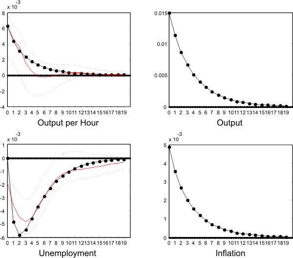
The dotted lines in Figure ![]() and
and ![]() show the simulated impulse response functions
of productivity, unemployment, output and inflation to a technology and a monetary policy shock.
show the simulated impulse response functions
of productivity, unemployment, output and inflation to a technology and a monetary policy shock.
Following a positive technology shock, real money balances (i.e. aggregate demand) do not increase as much as productivity because prices are sticky and because the central bank does not accommodate the shock. As a result, aggregate demand is sticky in the short run. Being more productive, firms initially meet their demand by decreasing hours and effort since employment is a state variable. Measured labor productivity undershoots its new long-run level because of short-run increasing returns to hours. With shorter hours and lower effort, the value of a marginal worker (i.e. the reduction in labor costs achieved with an extra worker) goes down, firms post fewer vacancies, and unemployment increases. As prices adjust to the new productivity level, both labor margins return to their long run values.
Following a positive monetary policy shock, firms increase their labor input in order to satisfy demand. Again, since they must first rely on the intensive margin, measured labor productivity initially increases as hours and effort increase. With higher hours and effort, the value of a marginal
worker goes up, firms post more vacancies and unemployment goes down. As prices adjust to the new money supply level, both labor margins return slowly to their long run values. Finally, as we saw in Section ![]() , the interaction of nominal frictions and hiring frictions can generate a strong propagation mechanism: output and inflation show persistent responses to a monetary shock despite a low degree of nominal rigidity.
, the interaction of nominal frictions and hiring frictions can generate a strong propagation mechanism: output and inflation show persistent responses to a monetary shock despite a low degree of nominal rigidity.
Apart from a slight departure from the 95% confidence interval for the unemployment response, the model is remarkably successful at matching the empirical responses. Moreover, the model's output response to a technology shock is similar to the empirical response reported by Galí (1999).
5.3 The sign switch of 
In Section 2, I argue that two events could be responsible for the large increase in ![]() in the mid-80s: (a) a decline in the relative importance (or volatility) of non-technology shocks
versus technology shocks, and (b) a structural change in the transmission mechanism of shocks. In this subsection, I test whether they can quantitatively explain the magnitude of the change in
in the mid-80s: (a) a decline in the relative importance (or volatility) of non-technology shocks
versus technology shocks, and (b) a structural change in the transmission mechanism of shocks. In this subsection, I test whether they can quantitatively explain the magnitude of the change in ![]() .
.
5.3.1 Changes in the volatility of shocks
In Section 2, I document a large drop in the volatility of non-technology shocks relative to technology shocks and present some evidence suggesting that changes in the relative size of technology and non-technology shocks drive fluctuations in ![]() . To explore whether the volatility movements around 1980 are quantitatively large enough to explain the sign flip of
. To explore whether the volatility movements around 1980 are quantitatively large enough to explain the sign flip of ![]() , I use
my calibrated model to simulate the impact of a drop in the volatility of aggregate demand shocks on the correlation between productivity and unemployment. I generate unemployment and productivity series using technology and monetary innovations with standard deviations following step functions
that mimic the volatility movements that occurred around 1980. Figure
, I use
my calibrated model to simulate the impact of a drop in the volatility of aggregate demand shocks on the correlation between productivity and unemployment. I generate unemployment and productivity series using technology and monetary innovations with standard deviations following step functions
that mimic the volatility movements that occurred around 1980. Figure ![]() depicts the step functions used in the simulation. The validity of this approach is subject to the correct identification
and separation of technology and non-technology shocks. There is reassuring evidence (see Galí and Rabanal, 2004) that technology shocks are correctly identified by long run restrictions but, since I emphasize the role played by aggregate demand shocks, I also look at the Romer and Romer
(2004) monetary shocks. Those shocks are identified with a different method, but we can see in Figure
depicts the step functions used in the simulation. The validity of this approach is subject to the correct identification
and separation of technology and non-technology shocks. There is reassuring evidence (see Galí and Rabanal, 2004) that technology shocks are correctly identified by long run restrictions but, since I emphasize the role played by aggregate demand shocks, I also look at the Romer and Romer
(2004) monetary shocks. Those shocks are identified with a different method, but we can see in Figure ![]() that, notwithstanding the large volatility increase in the late 70s, their volatility
in 1975 is twice as high as that in 1990, a volatility drop similar to the one used in the simulation.
that, notwithstanding the large volatility increase in the late 70s, their volatility
in 1975 is twice as high as that in 1990, a volatility drop similar to the one used in the simulation.
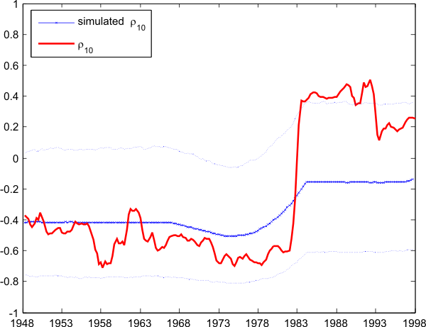
I simulate 60 years of data for unemployment and productivity. After filtering the (non-stationary) productivity series, I can calculate
![]() , the simulated 10-year rolling correlation between simulated productivity and unemployment. I repeat this exercise 5000 times to obtain the empirical distribution of
, the simulated 10-year rolling correlation between simulated productivity and unemployment. I repeat this exercise 5000 times to obtain the empirical distribution of
![]() . As shown in Figure
. As shown in Figure ![]() ,
,
![]() increases by around
increases by around ![]() and explains about 40% of the total increase
in
and explains about 40% of the total increase
in
![]() . In addition,
. In addition,
![]() overestimates
overestimates
![]() until 1980 and underestimates
until 1980 and underestimates
![]() afterwards, lying marginally inside the 95% confidence interval.23 If a drop in aggregate demand volatility seems to be part of the story, something else contributed to the sign switch in the mid 80s.
afterwards, lying marginally inside the 95% confidence interval.23 If a drop in aggregate demand volatility seems to be part of the story, something else contributed to the sign switch in the mid 80s.
5.3.2 Structural changes
In Section 2, I argued that two structural changes could be responsible for the large movement in ![]() in the mid-80s: (a) the central bank became more accommodating to technology shocks
after 1984, and (b) the procyclicality of measured labor productivity declined after 1984. In my model, a decrease in the procyclicality of productivity appears as a decrease in
in the mid-80s: (a) the central bank became more accommodating to technology shocks
after 1984, and (b) the procyclicality of measured labor productivity declined after 1984. In my model, a decrease in the procyclicality of productivity appears as a decrease in ![]() , the
short run returns to hours. Explicitly modeling a decrease in
, the
short run returns to hours. Explicitly modeling a decrease in ![]() is beyond the scope of the model but it would still be interesting to test if the decrease in the procyclicality of
productivity is enough to account for the sign flip of
is beyond the scope of the model but it would still be interesting to test if the decrease in the procyclicality of
productivity is enough to account for the sign flip of ![]() . I estimate the value of
. I estimate the value of ![]() and
and ![]() for each sub-sample, and I find that
for each sub-sample, and I find that ![]() decreased from
decreased from ![]() to
to ![]() between 1948-1983 and 1984-2005, while
between 1948-1983 and 1984-2005, while ![]() increased from
increased from ![]() to 0.
to 0.
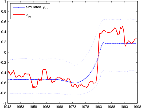
To study the impact of more accommodating monetary policy and less procyclical productivity on ![]() , I proceed as previously and simulate 60 years of data for
unemployment and productivity but allowing for different
, I proceed as previously and simulate 60 years of data for
unemployment and productivity but allowing for different ![]() and
and ![]() over
the two sub-periods as well as a drop in the volatility of monetary policy shocks. As shown in Figure
over
the two sub-periods as well as a drop in the volatility of monetary policy shocks. As shown in Figure ![]() ,
,
![]() increases this time from around
increases this time from around ![]() to
to ![]() , lies comfortably within the 95% confidence interval and does not over overestimate
, lies comfortably within the 95% confidence interval and does not over overestimate
![]() before the 80s.
before the 80s.
A remaining question is why productivity became less procyclical after 1984. A possible answer lies with a change in the behavior of inventories. The covariance between inventory investment and sales switched sign in 1984 and turned from positive to negative. A negative covariance means that inventories are used to smooth production fluctuations. To satisfy demand in the short run, firms use their inventories and do not rely as much on the intensive labor margin. With short run increasing returns to hours, productivity is less procyclical. On the other hand, with a positive covariance, inventory investment increases with sales, and in the short run, firms use their intensive margin to satisfy demand and increase inventories. Productivity is more procyclical. Various explanations have been proposed to explain this change in the covariance. Kahn, McConnell and Perez-Quiros (2002) argue that the late 70s and early 80s were times of dramatic innovations in manufacturing technology and inventory management. This has facilitated using inventories to smooth production. Looking at the automobile industry, Ramey and Vine (2004) propose a different explanation after showing that the serial correlation of sales decreased after 1984. With more transitory shocks, firms can more easily allow for deviations from their desired inventory-sales ratio since they know that deviations will be short-lived. Again, this facilitates the use of inventories to smooth production.
6. Embodied Technology and creative destruction
In this section, I discuss an alternative interpretation of the empirical relationship between labor productivity and unemployment studied in Section ![]() . In this alternative, we could ignore
aggregate demand altogether and emphasize instead the Schumpeterian aspect of technological progress. Indeed Michelacci and Lopez-Salido (2007) and Canova, Michelacci and Lopez-Salido (2007) argue that a technology shock with a permanent impact on productivity may increase unemployment through
creative destruction. The introduction of new technologies brings about a simultaneous increase in the destruction of technologically obsolete jobs which prompts a contractionary period during which employment temporarily falls. In that framework, the sign flip of
. In this alternative, we could ignore
aggregate demand altogether and emphasize instead the Schumpeterian aspect of technological progress. Indeed Michelacci and Lopez-Salido (2007) and Canova, Michelacci and Lopez-Salido (2007) argue that a technology shock with a permanent impact on productivity may increase unemployment through
creative destruction. The introduction of new technologies brings about a simultaneous increase in the destruction of technologically obsolete jobs which prompts a contractionary period during which employment temporarily falls. In that framework, the sign flip of ![]() in the mid 80s could be due to an acceleration of creative destruction spawned by the Information Technology (IT) revolution. Put differently, technology was disembodied before 1984 but became more embodied with the IT
revolution, and there is no need to appeal to aggregate demand to explain the sign switch. However, I see a number of arguments suggesting that creative destruction is not the most plausible explanation.
in the mid 80s could be due to an acceleration of creative destruction spawned by the Information Technology (IT) revolution. Put differently, technology was disembodied before 1984 but became more embodied with the IT
revolution, and there is no need to appeal to aggregate demand to explain the sign switch. However, I see a number of arguments suggesting that creative destruction is not the most plausible explanation.
First, if technical progress had become more embodied, this should have appeared in the empirical impulse responses. But as we saw, technology shocks had a quantitatively smaller negative impact on unemployment after 1984; exactly the opposite of what more creative destruction would imply but consistent with an improvement in the conduct of monetary policy.
Second, in a world with creative destruction, when productivity increases, unemployment goes up temporarily because firms destroy old and less productive jobs. If technology had become more embodied after 1984, movements in the separation rate should contribute to a larger fraction of unemployment fluctuations. However, Shimer (2005b) finds that the proportion of unemployment fluctuations accounted for by variations in the separation rate actually decreased from 21% to only 5% after 1985.24
Moreover, with embodied technology, firms need to post vacancies to create new matches with the latest level of technology. Hence, an acceleration of creative destruction in the mid 80s could have caused the correlation between productivity and unemployment to become positive, but it could not
have caused the correlation between productivity and vacancies to become negative. In contrast, an explanation emphasizing the role of aggregate demand shocks is consistent with large movements in both correlations: when productivity increases because of a technology shock, aggregate demand does
not adjust immediately, firms post fewer vacancies, and unemployment goes up. Looking again at Figure ![]() , the 10-year rolling correlation of labor productivity and
vacancies displays a sign switch similar to
, the 10-year rolling correlation of labor productivity and
vacancies displays a sign switch similar to ![]() and favors the latter explanation.
and favors the latter explanation.
Finally, it is important to distinguish between embodiment in new jobs and embodiment in new capital. For example, technology may be embodied in capital but disembodied in jobs.25 In order to explain the sign switch of ![]() with creative destruction, technological progress needs to be embodied in new jobs. Studying the impact of productivity
growth on unemployment, Pissarides and Vallanti (2005) find that technology embodied in jobs and creative destruction play no role in the dynamics of unemployment.
with creative destruction, technological progress needs to be embodied in new jobs. Studying the impact of productivity
growth on unemployment, Pissarides and Vallanti (2005) find that technology embodied in jobs and creative destruction play no role in the dynamics of unemployment.
7. Conclusion
By studying the joint behavior of labor productivity and unemployment, I uncover a sign switch in their correlation that poses a puzzle to the MP model of unemployment. From negative, the correlation turned positive in the mid 80s. Further, using long run restrictions to identify technological innovations, I find that, contrary to what search models imply, a positive technology shock increases unemployment in the short run.
I present a model with hiring frictions, variable effort and costly price adjustment that can rationalize the empirical observations. In this framework, positive technology shocks temporarily raise unemployment because with costly price adjustment, aggregate demand does not increase as much as
productivity, and firms use less labor. The correlation between unemployment and productivity, ![]() , is positive. On the other hand, positive aggregate demand disturbances decrease unemployment
and increase productivity temporarily because firms increase workers' effort to satisfy demand in the short run. As a result,
, is positive. On the other hand, positive aggregate demand disturbances decrease unemployment
and increase productivity temporarily because firms increase workers' effort to satisfy demand in the short run. As a result, ![]() is negative. I document two new facts that can account for the
large and swift increase in
is negative. I document two new facts that can account for the
large and swift increase in ![]() in the mid 80s: (a) an increase in the size of technology shocks relative to other shocks, and (b) a decline in the procyclicality of measured productivity
since the mid 80s. Using a calibrated version of the model, I simulate the impact of these two events and find that they quantitatively explain the sign switch of
in the mid 80s: (a) an increase in the size of technology shocks relative to other shocks, and (b) a decline in the procyclicality of measured productivity
since the mid 80s. Using a calibrated version of the model, I simulate the impact of these two events and find that they quantitatively explain the sign switch of ![]() . I suspect that the
decrease in the procyclicality of labor productivity after 1984 is linked to a change in inventory management after 1984 but a precise examination would require a theoretical integration of capacity utilization decisions (such as workers' effort) and inventory decisions,
and I leave this task for future research.
. I suspect that the
decrease in the procyclicality of labor productivity after 1984 is linked to a change in inventory management after 1984 but a precise examination would require a theoretical integration of capacity utilization decisions (such as workers' effort) and inventory decisions,
and I leave this task for future research.
Finally, by explicitly considering the interaction between hiring frictions and nominal frictions and by allowing labor to adjust along the extensive and intensive margin, the model highlights a new propagation mechanism that originates in the trade-off existing between the two labor inputs: the extensive margin is less expensive than the intensive one in the long run but it is also less flexible because of hiring frictions. In this setup, I show that the volatility of unemployment and the persistence of inflation increase with the magnitude of the trade-off.
Bibliography
Altig D., L. Christiano, M. Eichenbaum and J. Linde. "Firm -Specific Capital, Nominal Rigidities and the Business Cycle," Working Paper, 2004.
Andolfatto, D. "Business Cycles and Labor-Market Search," American Economic Review, 86(1), 1996.
Basu, S. and J. Fernald. "Aggregate productivity and aggregate technology," European Economic Review, vol. 46(6), pp. 963-991, 1997.
Basu, S. and M. Kimball. "Cyclical Productivity with Unobserved Input Variation," NBER Working Papers 5915, 1997.
Basu, S., J. Fernald and M. Kimball. "Are Technology Improvements Contractionary?," NBER Working Papers 10592, 2004.
Bils, M. and J. Cho. "Cyclical Factor Utilization," Journal of Monetary Economics, 33, 319-354, 1994.
Bils, M. and P. Klenow. "Some Evidence on the Importance of Sticky Prices," Journal of Political Economics, 112(5), pp. 947-985, 2004.
Blanchard, O. and P. Diamond, "The Beveridge Curve," Brookings Papers on Economic Activity 1, pp. 1-60, 1989.
Blanchard, O. and J. Galí. "A New Keynesian Model with Unemployment ," Working Paper, 2006.
Blanchard, O. and D. Quah. "The Dynamic Effects of Aggregate Demand and Supply Disturbances,", American Economic Review, 79(4), 655-673, 1989.
Blanchard, O. and J. Simon. "The Long and Large Decline in U.S. Output Volatility," Brookings Papers on Economic Activity 1, pp. 135 - 164, 2001.
Braun, H., R. De Bock and R. DiCecio, "Aggregate Shocks and Labor Market Fluctuations," Federal Reserve bank of St. Louis Working Paper, 2006.
Canova, F., C. Michelacci and D. López-Salido, "Schumpeterian Technology Shocks," mimeo CEMFI, 2007.
Christoffel, K., K. Kuester and T. Linzert " Identifying the Role of Labor Markets for Monetary Policy in an Estimated DSGE Model," ECB Working Paper No 635, 2006.
den Haan, W., G. Ramey and J. Watson. "Job Destruction and Propagation of Shocks," American Economic Review, 90(03), 2000.
Fernald, J. "Trend Breaks, long run Restrictions, and the Contractionary Effects of Technology Shocks," Working Paper, 2005.
Fisher, J. "The Dynamic Effects of Neutral and Investment-Specific Technology Shocks," Journal of Political Economy, 114(3), 2006.
Francis, N. and V. Ramey, "The Source of Historical Fluctuations: An Analysis using long run Restrictions," NBER International Seminar on Macroeconomics, 2004.
Galí, J. "Technology, Employment and The Business Cycle: Do Technology Shocks Explain Aggregate Fluctuations?," American Economic Review, 89(1), 1999.
Gali, J. and L. Gambetti. "On the Sources of the Great Moderation," Universitat Pompeu Fabra Working Paper 1041, 2007.
Galí, J., D. López-Salido and J. Vallés. "Technology Shocks and Monetary Policy: Assessing the Fed's Performance," Journal of Monetary Economics, vol 50, pp. 723-743, 2003.
Galí, J and P. Rabanal. "Technology Shocks and Aggregate Fluctuations: How Well Does the RBC Model Fit Postwar U.S. Data?," NBER Macroeconomics Annual, 2004.
Gertler, M. and A. Trigari "Unemployment Fluctuations with Staggered Nash Wage Bargaining," Working Paper 2006.
Hall, R. "Employment Fluctuations with Equilibrium Wage Stickiness," American Economic Review, 95(1), pp. 50-65, 2005.
Hall, R. "Job Loss, Job Finding, and Unemployment in the U.S. Economy over the Past Fifty Years," NBER Macroeconomics Annual, pp. 101-137, 2005.
Kahn, J., M. McConnell, G. Perez-Quiros. "On the Causes of the Increased Stability of the U.S. Economy," FRBNY Economic Policy Review, 183 - 202, 2002.
Krause, M and T. Lubik. "The (Ir)relevance of Real Wage Rigidity in the New Keynesian Model with Search Frictions", Journal of Monetary Economics, 54 pp. 706-727, 2007.
López-Salido, D. and C. Michelacci "Technology Shocks and Job Flows", CEMFI WP 0405, 2006.
Mertz, M. "Search in the Labor Market and the Real Business Cycle," Journal of Monetary Economics, 49, 2002.
Michelacci, C. and D. López-Salido, " Technology Shocks and Job Flows," Review of Economic Studies, 74, 2007.
Mortensen, D. and E. Nagypal. "More on Unemployment and Vacancy Fluctuations," NBER Working Papers 11692, 2005.
Mortensen, D and C. Pissarides. "Job Creation and Job Destruction in the Theory of Unemployment," Review of Economic Studies,61, 397-415, 1994.
Pissarides, C. "Search, Wage Bargains and Cycles," Review of Economic Studies, 54, 473-83, 1987.
Pissarides, C. Equilibrium Unemployment Theory, 2nd ed, MIT Press, 2000.
Pissarides, C. and G. Vallanti. "The Impact of TFP Growth on Steady-State Unemployment," International Economic Review, Forthcoming, 2005.
Ramey, V. and D. Vine. "Declining Volatility in the U.S. Automobile Industry," American Economic Review, Forthcoming.
Ravenna, F. and C. Walsh, "Vacancies, Unemployment, and the Phillips Curve," Kiel Working Papers 1362, 2007.
Schor J., "Does Work Intensity Respond to Macroeconomic Variables? Evidence from British Manufacturing," Working Paper, 1987.
Shapiro, M. and M.Watson. "Sources of Business Cycle Fluctuations," NBER Macroeconomics Annual, pp. 111 - 148, 1988.
Shimer, R. "The Cyclical Behavior of Equilibrium Unemployment and Vacancies," American Economic Review, 95(1), pp. 25-49, 2005.
Shimer, R. "The Cyclicality of Hires, Separations, and Job-to-Job Transitions," Federal Reserve Bank of St. Louis Review, 87(4), pp. 493-507, 2005.
Shimer, R. "Reassessing the Ins and Outs of Unemployment," NBER Working Paper No. 13421, 2007.
Stock, J. and M. Watson. "Has the Business Cycle Changed and Why?", NBER Macroeconomics Annual, 2002, pp. 159 - 218.
Stock, J. and M. Watson. "Has the Business Cycle Changed? Evidence and Explanations," FRB Kansas City symposium, Jackson Hole, Wyoming, August 28-30, 2003.
Trigari, A. "Labour Market Search, Wage Bargaining and Inflation Dynamics," IGIER Working Paper, 2004.
Walsh, C. "Labor Market Search and Monetary Shocks," in Elements of Dynamic Macroeconomic Analysis, S. Altug, J. Chadha, and C. Nolan, Cambridge University Press, 2004, 451-486.
Woodford, M. "Inflation and Output Dynamics with Firm-Specific Investment," Working Paper, 2004.
| 1948-1984 | 1985-2007 | |
| -0.31** | 0.46** | |
(Standard Error) |
(0.11) | (0.18) |
| 0.34** | -0.19 | |
(Standard Error) |
(0.14) | (0.17) |
Note: Table 1 reports estimates of the correlation between unemployment and labor productivity over 1948:Q1-1984:Q4 and 1985:Q1-2007:Q4, and between vacancies and labor productivity over 1951:Q1-1984:Q4 and 1985:Q1-2007:Q4. All series are detrended with an HP-filter with smoothing parameter 1600. Standard-errors are shown in parentheses. Significance is indicated by one asterisk (10-percent level) or two asterisks (5-percent level).
 |
 |
 |
 |
 |
 |
 |
 |
 |
 |
 |
 |
 |
 |
 |
Estimation of technology and non-technology shocks
I am interested in estimating the system
where
Without loss of generality, (12) can be written
 |
||
 |
As discussed in Shapiro and Watson (1988), imposing the long run restriction that only technology shocks have a permanent effect on
 |
(13) | |
 |
(14) |
Since
(Non-stationary) Equilibrium
In this non-stationary model economy, I rescale the non-stationary variables with the technology index ![]() Denoting rescaled variables with lower-case letters, the frictionless economy
is described by the following system with 5 equations and 5 unknowns
Denoting rescaled variables with lower-case letters, the frictionless economy
is described by the following system with 5 equations and 5 unknowns
![]() ,
, ![]() ,
, ![]() ,
, ![]() and
and ![]() :
:
 |
||
 |
||
 |
||
 |
where
An equivalent model with Calvo price setting
In this section, I describe a model similar to the one presented on Section 3 but with the assumption of Calvo price setting instead of costly price adjustment. Specifically, firms can only reset their price (at no cost) at random dates, and each period a fraction ![]() of randomly selected firms cannot reset its price.
of randomly selected firms cannot reset its price.
Since the job posting condition remains unchanged, I do not repeat it here. With Calvo-type price setting however, the optimal price setting rule is different, and a firm resetting its price at date ![]() will satisfy the standard Calvo price setting condition:
will satisfy the standard Calvo price setting condition:
![\displaystyle E_{t}\sum_{j=0}^{\infty}\nu^{j}\beta_{j}\left[ \frac{P_{it}^{\ast}}{P_{t+j}% }-\mu s_{it+j}\right] Y_{t+j}P_{t+j}^{\varepsilon}=0](img242.gif)

To derive the New-Keynesian Phillips curve, I log-linearize around the zero inflation equilibrium. However, because of firms' ex-post heterogeneity, the derivation is not as straightforward as with costly price adjustment. I follow Woodford's (2004) similar treatment of endogenous capital in a
New-Keynesian model with Calvo price rigidity. In my case, employment is the state variable and plays the role of capital in Woodford's model. I start by log-linearizing the first-order conditions around the zero-inflation equilibrium. For any ![]() , the vacancy posting condition becomes
, the vacancy posting condition becomes
with the value of a marginal worker

with
The notation
Denoting log prices by lower-case letters and
Averaging across all firms, I get
where
 is the average price chosen by all price setters at date
 With Calvo price-setting, I can write

 . Further,
 .
.Averaging (17) across all firms, I can rewrite the real marginal cost as
where
Using that
Moreover, subtracting (15) from its average, I get
since
The firm's pricing decision depends on its employment level and the economy's aggregate state. But to a first order, the log-linearized equations are linear so that the difference between
with
with
Subtracting (23) from its average, I obtain
This equation is of the conjectured form (22) if and only if
Finally, averaging (23) and using
Hence, a model with a Calvo price setting mechanism is described by the same log-linearized first-order conditions as a model with costly price adjustment.
![\displaystyle \left( \begin{array}[c]{c}% \Delta x_{t}\\ u_{t}% \end{array} \right) =C(L)\left( \begin{array}[c]{c}% \varepsilon_{t}^{a}\\ \varepsilon_{t}^{m}% \end{array} \right) =C(L)\varepsilon_{t}%](img19.gif)


![\displaystyle \frac{c_{t}}{q(\theta_{t})}=E_{t}\beta_{t+1}\left[ \chi_{it+1}+\frac{c_{t+1}% }{q(\theta_{t+1})}(1-\lambda)\right]%](img133.gif)


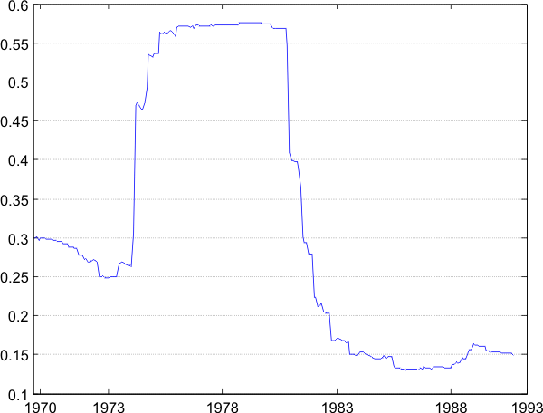
![\displaystyle \left( \begin{array}[c]{c}% \Delta x_{t}\\ u_{t}% \end{array} \right) =C(L)\left( \begin{array}[c]{c}% \varepsilon_{t}^{a}\\ \varepsilon_{t}^{d}% \end{array} \right) =C(L)\varepsilon_{t}%](img211.gif)
![\displaystyle \frac{c\eta}{q(\theta^{\ast})}\hat{\theta}_{t}=E_{t}\beta\left[ \chi^{\ast }\hat{\chi}_{it+1}+\frac{c(1-\lambda)\eta}{q(\theta^{\ast})}\hat{\theta}% _{t+1}\right]%](img249.gif)
![\displaystyle % {\displaystyle\sum\limits_{k=0}^{\infty}} (\nu\beta)^{k}\hat{E}_{t}^{i}\left[ \tilde{p}_{it+k}-\hat{s}_{it+k}\right] =0%](img252.gif)


![\displaystyle =\hat{y}_{t+1}-\varepsilon\left[ \nu(% {\displaystyle\int\limits_{0}^{1}} p_{it}di-p_{t+1})+(1-\nu)(% {\displaystyle\int\limits_{0}^{1}} p_{it+1}^{\ast}di-p_{t+1})\right]](img261.gif)

![\displaystyle \left( 1+\varepsilon\left( \frac{1+\sigma_{h}}{\varphi}-1\right) \right) p_{it}^{\ast}=\left( 1-\nu\beta\right) {\displaystyle\sum\limits_{k=0}^{\infty}} (\nu\beta)^{k}\hat{E}_{t}^{i}\left[ \hat{s}_{t+k}+\left( 1+\varepsilon \left( \frac{1+\sigma_{h}}{\varphi}-1\right) \right) p_{t+k}-\left( \frac{1+\sigma_{h}}{\varphi}-1\right) \tilde{n}_{it+k}\right]%](img272.gif)
![\displaystyle \phi p_{it}^{\ast}=\left( 1-\nu\beta\right) {\displaystyle\sum\limits_{k=0}^{\infty}} (\nu\beta)^{k}\hat{E}_{t}^{i}\left[ \hat{s}_{t+k}+\left( 1+\varepsilon \left( \frac{1+\sigma_{h}}{\varphi}-1\right) \right) p_{t+k}\right] -(1-\nu\beta)\left( \frac{1+\sigma_{h}}{\varphi}-1\right) \tilde{n}% _{it}%](img285.gif)

