Heterogeneous Car Buyers: A Stylized Fact
JEL Codes: E01, E31
Prices for light vehicles tend to fall over their model year, and retrace those declines when next year's models are introduced. Using a new dataset, we document that the characteristics of car buyers vary significantly over the model year as well: as average prices of vehicles fall over the model year, so does the average income of the buyers. Under the assumption that income is negatively correlated with price sensitivity, our results show that price-insensitive consumers buy early in the model year, with more price-sensitive consumers waiting until prices fall.
This empirical result suggests car dealers engage in price skimming (i.e. intertemporal price discrimination), introducing new models at a high price, selling to those willing to pay top dollar, and then lowering the price to sell to the remaining market segments. A large theoretical literature explores various facets of this practice but there is little empirical evidence (see Nair (2007)). However, there are other explanations for price declines over the model year,4 and we do not attempt to test between these competing stories. Rather, we point out that our findings have potentially important implications for price measurement.5 In particular, the heterogeneity in the data raises questions about the ability of standard matched-model methods to value quality improvements in new goods.
A description of the data and our main finding is provided in section 2, and the implications for price measurement are discussed in section 3.
2. Stylized Fact
Data on transaction prices and unit sales of new light vehicles at the make/model/model-year level (for example a 2001 Honda Accord) are from JDPower.6 The data cover virtually all make/model/model-year combinations (models for short) sold in the U.S. in our sample period, from late 1999 to 2003. The price data gives average transaction prices, net of cash rebates and financing incentives across all buyers in a month (consumers, firms and government);7 the unit counts are the number of consumers reporting the purchase of a vehicle. We aggregate the monthly data to quarterly to match timing with our buyer characteristics data.
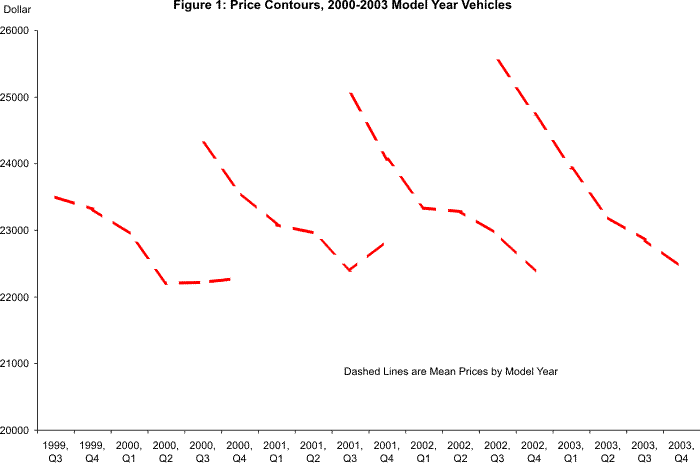
Figure 1 shows the average price for all models in a given model year in each quarter, for the 2000-2003 model years. The average price of these cars range from just above $22,000 to a bit below $26,000, with an evident decline over the model year. During our sample period, U.S. auto makers used incentives quite liberally; this trend was especially apparent in 2003, and these incentives account for much of the steep price decline seen that year. Figure 1 is not direct evidence that the prices of individual models are falling, on average, over the model year: the price of individual models may be constant, but more expensive models may be sold earlier in the model year. We consider this possibility below.
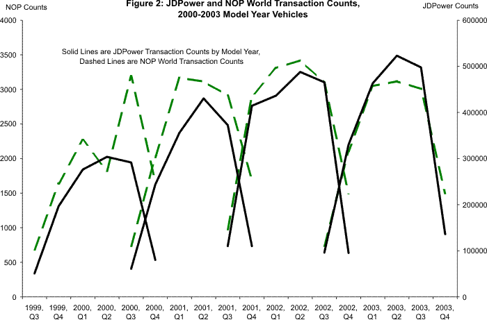
Data on the characteristics of car buyers is from surveys compiled by market data vendor NOPworld. Respondents to their questionnaire report whether they purchased a new vehicle in the previous 90 days. About half of NOP's questionnaires are sent out in the first month of the quarter; we assume respondents purchased their vehicles in the prior quarter. This classification system is not perfect, as some of these respondents may have purchased their vehicles in the same quarter they responded to the survey, rather than the prior quarter. Figure 2 shows, for each model year, the number of NOP transactions we attribute to each quarter, along with the sales counts from JDPower's database where the date of each sale is assigned accurately. The NOP data display approximately the same hump-shaped pattern in sales over the model year as the JDPower data, indicating our timing classifications are approximately accurate.
The make/model/model-year information in the NOP world data is self-reported and some responses do not correspond exactly with a JDPower make/model/mode-year category. In some cases we aggregate several NOP categories into a match with a JDPower category, but in most cases we have a one-to-one match between the two databases.
The annual household income of the buyer is reported by NOP in brackets, with widths of $5,000 for most brackets (for example the $25,000-$29,999 bracket) expanding to $50,000 at the top end of the distribution ($150,000-$199,999); we use the midpoint of each category as a proxy for the buyer's income.8 To ensure that these midpoints produce adequate proxies for income, we ran regressions of household income as measured by the midpoints on other demographic variables in the data set (such as the age and educational attainment of the household head), and found patterns quite similar to those exhibited in more widely-used surveys such as the Current Population Survey Annual Demographic Supplements and the Consumer Expenditure Surveys.
We assume that a household's income is an important determinant of its willingness to pay for a vehicle. A household's permanent income or consumption is probably better suited for this purpose. As a robustness check, we computed predicted values for income based on household heads' age, educational attainment, and other demographics. In the next section, we substituted these predicted values for the midpoints and obtained similar empirical results.
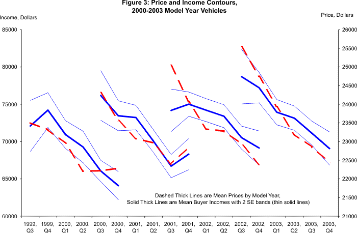
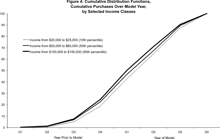
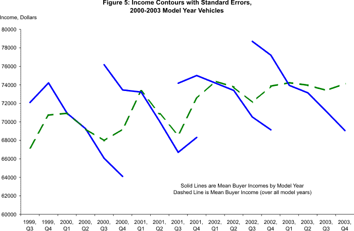
Figure 3 shows the main stylized fact of the paper, plotting the quarterly mean income of car buyers over each of the 2000-2003 model years, along with the corresponding contours for prices; two-standard error bands for the income means are also shown. Average buyer income falls substantially over the course of a model year along with the average car price. Getting at this fact from a slightly different angle, we computed cumulative distribution functions (CDFs) of car buyers by timing of purchase over the model year, for each income bracket. The CDFs of buyers in the lower-income brackets were generally below the CDFs of buyers in the higher-income brackets: lower-income buyers tend wait longer to buy a new car, buying later in the model year. This can be seen in Figure 4. The fall in average buyer income for buyers of a particular model year occurs despite the fact that the overall average income of car buyers in our sample trended up from late 1999 to the end of 2003 (shown in Figure 5).9
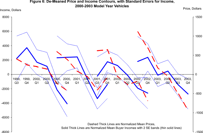
It is possible that more-expensive models are sold disproportionately earlier in the model year, and since the rich tend to buy these models more than the poor, this could explain the common fall in prices and buyers' incomes over the model year. To check that this is not the whole story - i.e. that the prices of individual models are falling on average, and that the income of buyers conditional on model type is falling on average as well - we ran regressions of average prices and incomes on a full set of make/model/model-year fixed effects, then averaged the residuals over makes/models in each model year. The resulting plot - Figure 6 - shows that eliminating the fixed effects associated with each make/model/model-year does not remove the downward sloping pattern that prices and income show over the model year. In other words, prices and buyer incomes continue to decline over the model year, holding the type of vehicle fixed. The changes in income from the fourth quarter of the year before the model year to the fourth quarter of the model year, for the 2000-2003 model years, are about $7800, $3800, $4400, and $5100, respectively, and these declines in average income are statistically significant, with t-statistics of 5.4, 2.7, 3.2, and 3.5, respectively.
With regard to periods where the two models overlap, in 2000Q4, households who bought 2001 model-year cars had about $6500 more income than households who bought 2000 model-year cars, and the t-statistic for this difference is 4.9 (Figure 6). In 2001Q4, households who bought the newer model-year had about $3100 more income (t-stat of 2.5), and in 2002Q4, newer model-year buyers had about $5000 more income (t-stat of 3.4). In each case, buyers of the newer model year cars have significantly higher income than buyers of the still-available older model year cars, after controlling for composition.
3. Implications for Price Measurement
Matched-model methods often translate the observed price declines for cars over the model year into rapid rates of quality improvement; the matched-model indexes of Corrado, Dunn and Otoo (2006) show an average quality improvement of 8% per year. An alternative method in Bils (2004) supports these magnitudes of quality improvements. However, while the BLS uses matched model indexes for some components of the CPI, it does not do so for cars. Instead, the BLS obtains estimates of quality improvements directly from firms, and their resulting price indexes fall much less rapidly.
Numerically, matched-model indexes account for quality change in two ways. Over the model year, the indexes control for quality change by tracking prices for identical goods. Our finding does not in and of itself present problems for measuring price change over the model year; as long as the goods may be considered identical, the price declines represent "pure price change" that will be properly recorded as such by the matched-model index. 10
The potential difficulty with buyer heterogeneity lies in the ability of matched-model methods to value quality improvements in new goods. When new models with potentially different characteristics are introduced, the matched-model method interprets any gap in prices for old and new models at a point in time as the market's valuation of the quality differences--differences in characteristics across goods (Aizcorbe 2006). This makes sense with a representative consumer that buys all goods every period; he was willing to pay all prices so that the gaps between them could reflect his value of the quality differences.
However, with heterogeneous consumers, this gap comingles differences in the price that arise from the fact that the goods are different--differences in quality--with those that arise because the buyers are different--differences in valuations across buyers. In the simplest case with only two goods, where an old good exits at time t and is replaced by a new good, the matched-model compares the prices of the new and old good to value the quality improvement in the new good.11 Literally, the gap in prices measures the difference between what price-insensitive buyers paid for the new good and what a price-sensitive buyers paid for the old good.
Suppose, instead, that one wanted a measure of the average valuation over all buyers in the market in that period. Intuitively, buyers of the old model were not willing to buy the new model at the market price, so the gap in prices probably overstates their valuation of the quality differences. However, the new-model buyers similarly did not want to buy the old model at the market price so the gap in market prices probably understates their valuation of the quality differences.12 Hence, it is not clear how one can tie the usual matched-model valuation to the valuations of the underlying buyers. Year-over-year price comparisons across model years may hold the characteristics of buyers more constant, alleviating the problems of buyer heterogeneity we have documented. But some alternative method for valuation of quality change must be employed in such comparisons, possibly hedonic regression.
References
Ana Aizcorbe, 2006. "Why Did Semiconductor Price Indexes Fall So Fast in the 1990s? A Decomposition," Economic Inquiry, Oxford University Press, 44(3):485-496, July.
Bils, Mark (2004). "Measuring Growth from Better and Better Goods," NBER Working Paper Series 10606. Cambridge, Mass., July.
Copeland, Adam, Wendy Dunn and George Hall (2004) "Prices, Production and Inventories over the Automotive Model Year." (FEDS Working Paper 2005-25)
Corrado, Carol, Maria Otoo and Wendy Dunn (2006) "Incentives and Prices for Motor Vehicles:What has been Happening in Recent Years?" (FEDS Working Paper 2006-09).
Erickson, Timothy and Ariel Pakes (2008) "An Experimental Component Index for the CPI: From Annual Computer Data to Monthly Data on Other Goods." Mimeo.
Nair, Harikesh (2007). "Intertemporal Price Discrimination with Forward-looking Consumers: Application to the US Market for Console Video-Games," Quantitative Marketing and Economics, 5(3):239-292.
Pakes, Ariel (2003) "A Reconsideration of Hedonic Price Indices with an Application to PCs." American Economic Review 93:1578-1596.
Pashigian, Peter, Brian Bowen, and Eric Gould (1995). "Fashion, Styling, and the Within-Season Decline in Automobile Prices," Journal of Law and Economics, 38:281-309.
