Skip to: [Printable Version (PDF)] [Bibliography] [Footnotes]

Finance and Economics Discussion Series: 2009-32 Screen Reader version ^♣

Improving Real-Time Estimates of the Output Gap

Thomas M. Trimbur*

Federal Reserve Board

April 2009

Keywords: Business cycles, Kalman filter, potential output, state space, stochastic cycles, unobserved components.

Abstract:

This paper investigates strategies for real-time estimation of the output gap. First, I examine estimates from univariate models with stochastic cycles. This corresponds to the use of model-based band-pass filters in real-time, and I find that the turning points in real-time and final output gap series match more closely for higher order models and that the revisions properties and real-time accuracy are more favorable. Second, I investigate the use of capacity utilization as an auxiliary indicator to improve on output gap estimates in real-time. I find that this bivariate approach leads to significant gains in the accuracy of real-time estimates and in the quality of revisions.

JEL classification: C22, E32.

Disclaimer: This report is released to inform interested parties of ongoing research and to encourage discussion of work in progress. The views expressed on statistical, methodological, technical, or operational issues are those of the authors and not necessarily those of the Federal Reserve Board.

1 Introduction

The measurement of the output gap, or position of the business cycle, is of central importance in discussions about the current state of the economy. As a summary indicator of aggregate demand conditions and economic performance, estimates of the output gap serve as a key input in policy-making. Updated assessments or policy decisions are made with the information available at the time, so attention centers on the real-time estimate of the output gap.

In studying macroeconomic fluctuations, current analysis reflects real-time data. Therefore, in accounting for agents' beliefs and their relationship with the economy, one must incorporate the proper knowledge at each time point. The evolution of the output gap is of particular interest as it signals the general economic climate and the potential for inflationary pressures. Yet recent work, such as Orphanides and Van Norden (2002) and Watson (2006), has highlighted the challenges in getting useful and accurate estimates in real-time. The importance of real-time analysis has been exemplified in the work of Orphanides (2001), who showed that basic conclusions about the stance of monetary policy can be affected. Orphanides and Van Norden (2002) compared a number of methods for estimating output gaps and concluded that none of the methods was particularly reliable, in the sense that revisions were excessively large and had undesirable properties.

In this paper, I try a different approach along two separate dimensions. First, I produce the real-time estimates of the output gap from time series models that explicitly account for cyclical behavior. Second, I investigate the strategy of using capacity utilization as an auxiliary indicator to improve on these estimates.

Recently, a class of unobserved components models has been proposed by Harvey and Trimbur (2003). The implied filters for such models give rise to a class of low-pass and band-pass filters, related to the well-known Butterworth filters in engineering. The filters generated by the model are consistent with each other and with the data, and thus, one of their prime advantages is the coherency of the output gap estimates that are produced. Another advantage is that they automatically adapt to the ends of the sample. The "ideal filter", or perfectly sharp filter, which has been emulated in applied work such as Baxter and King (1999) and Christiano and Fitzgerald (2003), emerges as a limiting case of the model-based filters. Harvey and Trimbur (2003) fit the models to US real GDP and investment and show how the higher order models lead to smoother cycles. The implied band-pass filters taper off gradually at the frequency endpoints. One goal in this paper is to investigate the application of the models and associated band-pass filters in real-time.

Another goal is to examine the ability of capacity utilization as an indicator for the output gap. Capacity utilization (CU) is a broad indicator of economic activity that has clear cyclical properties and that has close links with a number of major economic variables, such as the inflation rate. The use of additional series to help improve estimates of trend, or potential has been demonstrated recently in Basistha and Startz (2007), who relate cyclical components in different series to get a more accurate estimate of the natural rate of unemployment. Watson (2006) also finds some improvement in combining series with economic content, or information about the business cycle, in real-time estimation. In another study, Planas and Rossi (2004) use inflation data to improve real-time estimates of the output gap. One motivation for using capacity utilization is that it is well known to represent a highly procyclical indicator. Another motivation is that macroeconomic theory, such as the real business cycle models in Burnside and Eichenbaum (1996) and Boileau and Normandin (2003), suggest a close connection with variations in output.

The Federal Reserve Board publishes industrial production, capacity, and capacity utilization measures for the U.S. industrial sector, which includes manufacturing, mining, and utilities. For a summary of the measurement of capacity utilization and a discussion of its role as a business cycle indicator, see Corrado and Mattey (1997). For more detailed information on the calculation of capacity and utilization from the source survey data, see Morin and Stevens (2003).

Capacity is defined as a realistically sustainable maximum level of output. This definition, involving the full use of available factors of production, has a close connection with the concept of potential output. As the rate of utilization measures the deviation of current activity from its capacity, or potential activity, it naturally helps indicate the position of the business cycle, or output gap. Despite this link with cyclical components, previous work on modeling and estimating the output gap has not considered capacity utilization as an indicator. In this paper, I attempt to fill this gap in the literature by examining how the rate of capacity utilization may be used in a real-time analysis to improve GDP gap estimation. As a precursor, a further aim is to investigate the cyclical dynamics of capacity utilization using structural time series models estimated in real-time.

The rest of the paper proceeds as follows. In Section 2, I discuss the real-time dataset on capacity utilization and apply a univariate time series model centered on a flexible cyclical component. In Section 3 I apply unobserved components models to quarterly real-time GDP and compare the results with those for capacity utilization. In Section 4 I first adapt the monthly real-time utilization data to the quarterly level, which requires careful consideration of data release timing, and then set up a bivariate model of real GDP and capacity utilization. The bivariate model is analyzed, and the properties of the real-time output gap estimates are measured and compared with earlier results. Section 5 concludes.

2 The cyclical behavior of Capacity Utilization

This section analyzes the real-time dataset on capacity utilization using an unobserved components approach. The stochastic cycle model is briefly reviewed, and estimates are first computed for the most recently available data to examine the overall characteristics of the series.

At each point in time, a particular sample, or vintage, is publicly available and represents the updated information available to the user of the data at that point in time. In real-time analysis, a distinction is made between the different vintages that have been available throughout the history of the dataset. The final estimates of the cycle are based on the latest vintage, or most recently available data. By comparing the real-time estimates with the final ones, the accuracy can be quantified, to assess how well the real-time estimates represent the final estimates, computed with the benefit of hindsight. Thus, the total revisions for the capacity utilization cycle are analyzed using several measures.

A primary focus of this paper is to improve real-time estimates of the GDP cycle, or gap. In choosing a useful indicator, I focus on capacity utilization for the manufacturing sector, which is the largest and most cyclical sector of production. Note also that earlier vintages are available for manufacturing utilization than for total industry utilization.

2.1 Real-time data

Data are taken from the real-time database of the Federal Reserve Bank of Philadelphia. The data on capacity utilization represents an expansion of the original real-time dataset for macroeconomics described in Croushore and Stark (2001). For CU, these vintages are recorded on a monthly basis, and the sample for each vintage extends to one month prior to the vintage month. For each vintage, labelled by month, the sample is assumed to include all information available by the end of the vintage month. The CU figures for a particular month are first released around the middle of the following month. For example, the earliest recorded vintage of the dataset for manufacturing CU is August 1979. This corresponds to the data available by the end of August, including the figures for July capacity utilization, which were originally released around the 15th of August. For all vintages up to August 2007 (the most recent vintage available at the time of writing), the recorded time series started in January 1969 or before. For consistency, in estimating models and components, I use a fixed starting point of January 1969.

The real-time estimate for a given month is based on data ending in that month (so the vintage is the following month), and each real-time estimate is revised a number of times with the arrival of information with each new vintage. In terms of vintage, the sample period for each vintage extends up to the month preceding the vintage month, so the most recent filtered estimate of the cyclical component, at the end of the sample period, also lies in the month preceding the vintage month; this gives the most timely indicator of the output gap. Thus, real-time estimation starts with the vintage of August 1979 (sample period from January 1969 to July 1979) and ends with the vintage of August 2007 (sample period from January 1969 to July 2007). In terms of comparing real-time and final estimates, the first cyclical estimate analyzed is July 1979, and the last cyclical estimate analyzed is May 2005. This allows for reasonable spacing, or duration, between final estimate and final vintage.

2.2 Modeling cyclical dynamics

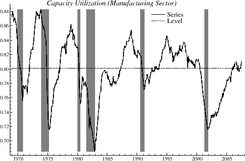
Figure 1 shows the data available in August 2007. Shaded regions indicate recessions as dated by the NBER. A simple inspection of the graph shows that it is highly cyclical, and in fact, many declines in the utilization rate foreshadowed or coincided with the onset of an economic downturn¹. As there is no obvious long-term trend in the series, a natural model to capture the cyclical behavior is given by

$\displaystyle y_{t}=\overline{\mu}+\psi_{n,t}+\varepsilon_{t}$ , $\displaystyle % \varepsilon_{t}\sim WN(0,\sigma_{\varepsilon}^{2}),$ $\displaystyle t=1,...,T %$

(1)

where

denotes `white noise', the parameter $\overline{\mu}$ represents an average level, and $\psi_{n,t}$ is an

th order stochastic cycle.

This class of cyclical models, introduced in Harvey and Trimbur (2003), is defined as²

$\displaystyle \left[ \begin{array}[c]{l}% \psi_{1,t}\\ \psi_{1,t}^{\ast}% \end{array} \right] =\rho\left[ \begin{array}[c]{ll}% \cos\lambda_{c} & \sin\lambda_{c}\\ -\sin\lambda_{c} & \cos\lambda_{c}% \end{array} \right] \left[ \begin{array}[c]{l}% \psi_{1,t-1}\\ \psi_{1,t-1}^{\ast}% \end{array} \right] +\left[ \begin{array}[c]{c}% \kappa_{t}\\ \kappa_{t}^{\ast}% \end{array} \right]%$

(2)

$\begin{displaymath} \left[ \begin{array}[c]{l}% \psi_{i,t}\ \psi_{i,t}^{\ast}% \end{array}\right] =\rho\left[ \begin{array}[c]{ll}% \cos\lambda_{c} & \sin\lambda_{c}\ -\sin\lambda_{c} & \cos\lambda_{c}% \end{array}\right] \left[ \begin{array}[c]{l}% \psi_{i,t-1}\ \psi_{i,t-1}^{\ast}% \end{array}\right] +\left[ \begin{array}[c]{c}% \psi_{i-1,t-1}\ \psi_{i-1,t-1}^{\ast}% \end{array}\right] ,\quad i=2,...,n \end{displaymath}$

where $\kappa_{t},\kappa_{t}^{\ast}\sim WN(0,\sigma_{\kappa}^{2})$ and $\kappa_{t}$ is uncorrelated with $\kappa_{t}^{\ast}$ . Note that $\kappa_{t}$ and $\kappa_{t}^{\ast}$ are assumed uncorrelated with $\varepsilon_{t}%$ . The parameter $\rho$ is called the damping factor; it satisfies $0<\rho\leq1$ , while $0\leq\lambda_{c}\leq\pi$ . The central frequency of oscillation is $\lambda_{c}$ , with corresponding period of 2 $\pi/\lambda_{c}$ .

The model in (2) guarantees a peaked spectral shape, with a certain width, for suitable parameter values. This shape characterizes cyclical behavior in economics where, in the frequency domain, a spectrum displaying a clear peak indicates a tendency for periodic movements. Relative to engineering or the physical sciences, one typically would expect a wider peak because, for economic series, random disturbances of different kinds play a relatively more important role. For , the shocks on the right hand side of the recursion in (2) are themselves cyclical; this gives rise to a kind of resonance effect, reinforcing the cycle. Harvey and Trimbur (2003) found that higher order models were especially appropriate for US investment, a series known to have a pronounced cyclical component.

One advantage of (2) is that the model parameters are directly linked to cyclical behavior; periodicity may be studied directly, for instance, through $\lambda_{c}$ . An advantage of the models $\psi_{n,t},$ with , is that they allow for estimation of smoother cycles, which can be useful for studying turning points. General expressions for the autocovariances and spectrum are given in Trimbur (2006). The spectral shape shows increased concentration around the central frequency as increases.

Estimation results for different orders are shown in table 1 for the most recent vintage for CU. I estimate the models by ML using state space methods; this requires the stronger assumption of Gaussian disturbances. Given a feasible parameter vector, the likelihood function is evaluated from the prediction error decomposition obtained from the Kalman filter, see Harvey (1989). The parameter estimates are computed by optimizing over the likelihood surface in each case. To do the calculations for the results given below, programs were written in the Ox language (Doornik 2006) and included the Ssfpack library of state space functions (Koopman et. al 1999). Several diagnostics are reported in the table. $R_{D}^{2}$ is the coefficient of determination with respect to first differences, and $\widehat{\sigma}$ is the equation standard error. is the Box-Ljung statistic based on the first P residual autocorrelations. In all cases, I have set to the largest integer less than or equal to $\sqrt{T}$ where is the sample size. should be compared with a chi-squared distribution with degrees of freedom. The Akaike Information Criterion (AIC) is defined by $=-2\log\hat{L}+2k,$ where $\log\hat{L}$ is the maximized log-likelihood and is the number of model parameters.

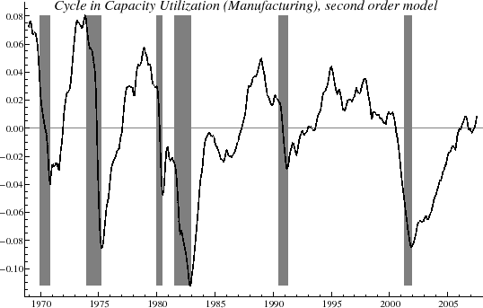
In figure 1, the level, $\overline{\mu}=0.800$ , indicated by the dotted line, was estimated with the cyclical model with . The component $\widetilde{\psi}_{2,t}$ is shown in figure 2; this indicates the cyclical oscillations above and below the mean level of utilization. The component $\widetilde{\varepsilon}_{t}$ represents the nonsystematic noise in the series and is graphed in figure 3. As $\widetilde{\varepsilon}_{t}$ is removed, $\widetilde{\psi}_{2,t}$ is smoother than the original series, and it is easier to make comparisons with recession dates and, more generally, to study transitions in the cycle. The diagnostics suggest that and 3 are the preferred models. As increases, the estimated variance³ of the cycle $\sigma_{\psi}^{2}$ declines somewhat, though the change from order 1 to 6 is relatively moderate, being somewhat less than 25%. It is clear in table 1 that the value of $\rho$ falls with ; this owes to the resonance property of higher order cycles, where shocks are increasingly reinforced within the system. For , the noise assigned to the irregular increases as the order rises, and the implied band-pass filter has a sharper cutoff on the right.

Typically, periods between, say, 1 1/2 to 8 years are taken as representative of business cycle movements. For , the estimated period is about seven years, and the estimate of $\rho$ is close to 0.99, indicating substantial persistence in the cycle. For higher orders, there is difficulty in estimating a period within the business cycle interval due to irregularities in the finite sample likelihood. These results are consistent with the experience of Harvey and Trimbur (2003) where an excessively large period was obtained for real GDP for . This problem is successfully addressed in Harvey, Trimbur, and van Dijk (2007), where it is shown how a weakly informative prior reflecting business cycle expectations can help overcome flatness in the likelihood surface. The Bayesian approach, in addition to providing a practical solution to an irregular likelihood, is appealing from other standpoints as well. In the current paper, however, I use a frequentist approach, and I choose to fix the period for higher to the value estimated for (this value, equal to about seven years, is plausible for a business cycle period, and fixing the frequency effectively corresponds to using an extremely sharp prior in a Bayesian analysis).

In preparation for the real-time analysis, suppose that a researcher starts with the first recorded vintage in the Philadelphia Fed's dataset, which became available in August 1979. This covers data from January 1969 to July 1979, and the researcher would encounter the series shown in figure 4. This differs from the early portion of the later vintage sample shown in figure 1. Now suppose model (1) is estimated on the early vintage dataset. Results are given in table 2 for different orders .

Figure 4 shows oscillations in the cycle, above and below an estimated mean level of utilization, due to the first two major oil price shocks. It is notable that, although there are only two cyclical swings present in the sample, the model in (1) is still able to pick out plausible periods for both (slightly above four years) and (about seven years). The pattern of estimated $\rho$ with respect to order is similar to that in table 1. There is again difficulty in estimating periods for higher orders , so these results are based on fixing the period to the average of the first and second order periods, that is, 66.4. The model chosen on the basis of fit is again with other higher order models also performing well. The estimated variance of the cycle $\sigma_{\psi}^{2}$ is slightly higher for than for other orders, so that the second order component explains a greater proportion of overall movements. The main point of this exercise is that, when a researcher estimates the output gap in real-time, starting with the data in figure 4, estimation of the models in (1) are viable and further, the results show that a higher order model, in particular , would tend to be chosen at an early stage of estimation.

2.3 Real-time estimation of the CU cycle

The previous Section showed the results of fitting the stochastic cycle model to two different data vintages of capacity utilization. In this sub-Section, I extend the treatment to real-time estimation for the range of available vintages.

Repeated estimation over different vintages shows that is consistently the best performing model, as for the first and last vintage. When unrestricted estimation led to a period outside the business cycle range (2 to 8 years), the period is constrained to equal seven years, or 84 months; this value, lying with the proper interval, approximately matches the estimate for the first vintage for the best fitting model (. Figure 5 shows the real-time estimates for the second order cycle and compares them with the final estimates obtained for the most recent vintage of August 2007. Note that in some periods the real-time estimates lie below the final ones for several consecutive periods, such as in 1982 (this means that the real-time estimates reflected greater severity of the recession) and in 1995-2000, whereas in other periods, the real-time estimates are consistently higher, such as 1984-7. Overall, however, the real-time estimates track the final ones rather well.

The quality and accuracy of the real-time estimates, in representing the final measures, is quantitatively assessed in tables 3 and 4. Table 3 presents a number of statistics related to the size and accuracy of revisions. Table 4 compares the characteristics of the real-time and final cyclical estimates. The values in the tables may be compared with those reported in Orphanides and van Norden (2002) for various methods applied to real-time GDP gap estimation.

The relatively accurate real-time estimation of the capacity utilization cycle is confirmed by looking at the measure, which indicates the correlation between real-time and final estimates. The correlation of nearly 0.95 is well above the correlations computed for all eight methods investigated in Orphanides and van Norden (2002). Further, opposite signs are obtained for the final and real-time cycles less often, and the ratio, representing the noisiness of revisions relative to output gap signal, is lower in every case. The high real-time accuracy is consistent across different These findings are encouraging for the use of the CU cycle as a real-time indicator for the output gap.

Figure 6 shows the revisions over the vintage set for and . The revisions are highly persistent, as indicated by the first order autocorrelation, , of more than 0.95. There is no tendency, however, for the real-time estimates to perform worse around the recession times. In contrast, for the first three recessions shown, the revisions immediately preceding the downturn are relatively small. The graphs shows moderate upward revisions around the start of the 1980 recession (indicating better than expected rates of utilization) and moderate downward revisions around the start of the 2001 recession (worse than expected). The biggest revisions occur around 1983-85, which saw large, downward, and erratic adjustments; around 1992, for which there were large, upward changes over a limited time span; and between 1998 and 2000, when there is an interval of noisy, upward revisions. The revisions then switch sign in the year 2000. There is little difference between the revisions for and . Overall, on comparison with the results for the GDP gap shown in the next Section, the summary statistics imply that the real-time estimates for the capacity utilization cycle are relatively successful as they anticipate the final values with reasonable accuracy.

3 The cyclical behavior of real GDP

In this Section, I investigate to what extent univariate models, which explicitly account for cyclical behavior, can give useful real-time estimates of the output gap. It is useful to focus on the cycle since it represents systematic deviation from potential, or the gap with noise removed. These models are also of interest in that they give rise to filters with band-pass properties. These implied filters enable one to extract cycles in a way that is consistent with the properties of the series and with the other components in the model. Furthermore, as they adapt to sample endpoints automatically, they provide a natural candidate for generating real-time cycle estimates. In this Section, I first discuss the dataset and unobserved components models briefly and then study the properties of the real-time estimates and their revisions.

3.1 Real-time data

Data are available from the real-time database of the Federal Reserve Bank of Philadelphia. Each vintage for real GDP covers a specific quarter and refers to the data that were available by the middle of the quarter. Note that the first estimate of GDP for a particular quarter is typically released around the end of the first month of the following quarter and so is already available around the middle of the second month of the following quarter. For instance, take 1985Q4; this vintage contains data that were available by mid-November, and the last observation recorded is for 1985Q3. Similarly, for each vintage up to the most recent one (2007Q3), the dataset contains values up to the quarter immediately preceding the vintage quarter. For each vintage, data are available from 1947Q1. The real-time estimates are computed by taking, for each vintage, the last estimate of the cycle in the sample. The final estimates are all computed from the last vintage of 2007Q3.

3.2 Modeling cyclical dynamics

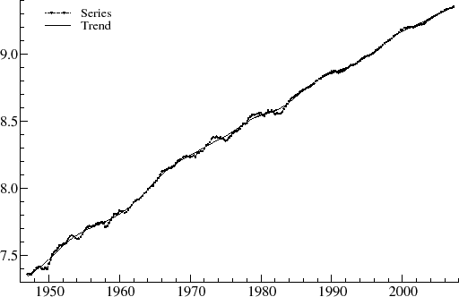
Figure 7 shows the latest vintage dataset for the logarithms of GDP. The graph shows cyclical movements around a clear upward trend.

The model fitted to the series is the following decomposition:

$\displaystyle y_{t}=\mu_{m,t}+\psi_{n,t}+\varepsilon_{t}$ , $\displaystyle \varepsilon _{t}\sim WN(0,\sigma_{\varepsilon}^{2}),$ $\displaystyle t=1,...,T %$

(3)

where $\psi_{n,t}$ is defined as before.

Now $\mu_{m,t}$ can be defined generally as an m-th order stochastic trend. Thus, given positive integer ,

$\displaystyle \mu_{1,t}^{{}}=\mu_{1,t-1}^{{}}+\zeta_{t}^{{}}%$

(4)

$\displaystyle \mu_{i,t}^{{}}=\mu_{i,t-1}^{{}}+\mu_{i-1,t}^{{}},\quad i=2,...,m$

where the disturbance term, $\zeta_{t}^{{}}\sim WN(0,\sigma_{\zeta}^{2})$ , is uncorrelated with $\varepsilon_{t}$ and with $\kappa_{t},\kappa_{t}^{\ast}$ . In what follows, I assume

, which gives the smooth trend model; this model underpins, for example, the well-known Hodrick-Prescott filter for smoothing a time series, and it is often used in structural time series models. Typically, in time series modelling,

or 2 as most series are

. The choice

has the advantage of producing smoother trends, which also makes it more feasible to estimate the cyclical behavior in a series. In the frequency domain, the resulting low-pass filter has a sharper cutoff at low frequencies.

The link of (3) with low-pass and band-pass filters was explored in Harvey and Trimbur (2003). Specifically, considering (3) as a signal extraction problem, the optimal estimator of the cycle is a filter with band pass properties applied to $y_{t}%$ ⁴. As increases the band pass filter tends toward a sharp filter, such as the one emulated in Baxter and King (1999)⁵.

Figure 7 is based on the model. The trend is clearly stochastic as there are changes in growth rate; for instance, potential output grew more quickly in the 1960's than in the 1970's. The fluctuations around the trend correspond to the changing output gap over the economic cycle, and these are shown in figure 8. The estimated period of the cyclical component is 2 $\pi/18.4$ , or about four and a half years.

Table 5 shows results for different orders for the last vintage, 2007Q3 (sample period from 1947Q1 to 2007Q2). These results may be compared with the estimates reported in Harvey and Trimbur (2003) for a sample period ending in 2001Q3. As in Harvey and Trimbur (2003), there is again difficulty in estimating a business cycle period for higher orders, so I fix the period for $n\geq2$ to the value obtained for . This difficulty, due to the flatness or irregularity of the likelihood, can also be overcome by the Bayesian approach in Harvey, Trimbur, and van Dijk (2007). In particular, one can specify an informative prior on the frequency, expressing expectations about the business cycle in a consistent way, and Bayesian modeling in real-time would provide other advantages, such as accounting for parameter uncertainty. In this paper, I retain a classical approach.

The estimation results in table 5 for the last vintage are basically similar to those in Harvey and Trimbur (2003). In addition to a period of between four and five years, for , the estimate of $\rho$ indicates a somewhat persistent cycle. The pattern of $\rho$ with respect to different is similar to that in tables 1 and 2, though the values are somewhat smaller for real GDP. Similar to the results for capacity utilization, as increases, the estimated variance $\sigma_{\varepsilon}^{2}$ rises as the irregular absorbs increasing amounts of noise from the cycle. In table 5, the cycle variance is relatively stable with respect to order, with $\sigma_{\psi}^{2}$ reaching a maximum for . The preferred models are 2 and higher with the second order doing best on the basis of $R_{D}^{2}$ and of AIC comparisons. For comparison, the estimated cycle for is shown in figure 8 along with the case.

In the next sub-Section, I will apply the model-based band-pass filters to real GDP in a real-time setting. As noted, the cyclical models have clear links with band-pass filters, but there is a key difference from the direct design of band-pass filters in the frequency domain. The intention of nonparametric methods, such as Baxter and King (1999) and Christiano and Fitzgerald (2003), is to select out the range of periods in an input process associated with the business cycle component, and the strategy is to emulate a particular shape of gain function. The interval of periods is chosen in advance, and further, the shape of the "ideal" filter is prespecified to be perfectly sharp. Although the concept is simple, this strategy involves a serious risk of properties distortion, as discussed, for instance, in Murray (2003) and Harvey and Trimbur (2003). Such distortions may, however, be avoided by designing a model-based band pass filter with the time series modelling approach. In this way, the cyclical component is estimated in a framework consistent with the data, and the filters for trends and cycles are also mutually consistent.

3.3 Real-time estimation of the GDP cycle

In a previous sub-Section, results were given for fitting the smooth trend plus stochastic cycle model to real GDP for the latest vintage, 2007Q3. Given the empirical performance of the models, their close connection with low-pass and band-pass filtering, and the availability of real-time data, I now investigate the use of the models and their associated filters in a real-time application.

Recall that the earliest vintage for monthly capacity utilization is August 1979; in transforming to a quarterly real-time dataset with quarterly vintages, the first vintage becomes 1979Q3 (discussed in the next Section). Now suppose a researcher estimating the output gap in real-time begins with the vintage of 1979Q3 for real GDP. The results of estimation are shown in table 6, and they have a similar form to the results in table 5. Thus, there is the same decline in $\rho$ with respect to , and the model is still preferred to . For the earlier vintage, however, a period in the business cycle range is estimated for both and 2, and the fit of the models for slightly improves on the fit for .

I now examine the real-time estimation of the GDP gap, with the different cyclical models, without using any information about the capacity utilization rate or other auxiliary indicators. In each case, the period, 2 $\pi/\lambda_{c}$ , is first estimated without restriction. If the resulting estimate lies outside the business cycle interval of two to eight years, then the period is constrained to equal five years, or 20 quarters; this nearly matches the average estimate for the first vintage for and 2, and the value falls near the center of the business cycle interval. For each quarterly vintage, the model is estimated and the most recent cyclical estimate is recorded as the real-time output gap. The last cyclical estimate analyzed is 2005Q2.

Tables 7 and 8 shows summary statistics for real-time estimates and revisions for the different cycle models. These results clearly differ from the results for capacity utilization given in tables 3 and 4, and they are typical of the results shown for different methods in Orphanides and van Norden (2002) for estimation of the GDP gap. The correlation between real-time and final estimates, which for capacity utilization was nearly 0.95, is now reduced to just above 0.50. Further, the values of are about three times higher for quarterly real GDP, and the frequency of matching signs is significantly reduced. On the other hand, the measure shows that the revisions to the GDP gap typically average about zero. The volatility, measured by and RMSE, decreases with order.

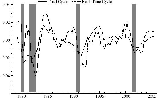
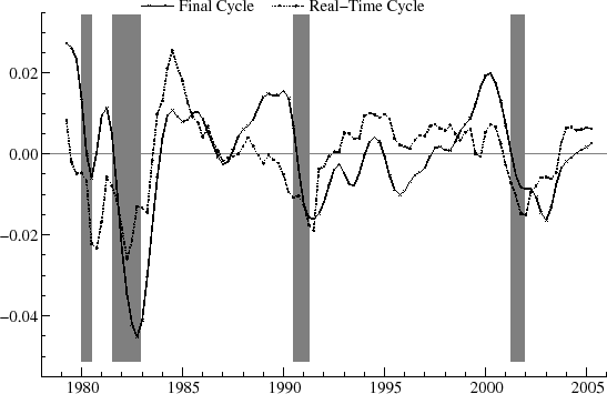
As an example, the real-time estimates of the output gap for are shown in figure 9 and for in figure 10. The relationship between the real-time and final estimates varies significantly over the historical period. At certain times, such as near the end of 1981 and during 1986, for they match up reasonably well. Over a number of intervals, however, there are clear differences. For instance, in 1989, the real-time estimate is negative and falling, while the final estimates are positive and stable. Also, in the mid-90's, the real-time estimates are often of opposite sign than the final estimates. Despite the sometimes large revisions, it appears that, with , the turning points in the real-time estimates roughly coincide with the turning points in the final estimates on a number of occasions. For instance, for , the downturn in the cycle marking the start of the 1981-2 recession is apparent in both real-time and ex post. Similarly, the recovery beginning after the 90-91 recession is evident in both series, and the decline in the cycle around 2000-1 starts at the same point in both real-time and final estimates. These turning points show up more clearly for than for .

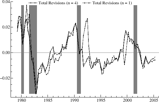
Figure 11 compares the revision history for and 4. The revisions tend to track each other, though one exception is that there is a large upward revision for several quarters in 1991-2 for , whereas for the revision is downward and of more moderate size. For each of the first three recesions, the revisions show a tendency to decrease as the downturn in the cycle progresses. The revisions show a fairly steady increase from about 1983 to 1990; from around 1984 to 1987, the revisions are larger in magnitude for the first order model. Generally, the revisions are highly persistent, for example remaining negative throughout much of the 1990's. Compared to those for , typically, the revisions for appear less volatile (note the lower and RMSE in table 7 and the lower in table 8) and slightly more persistent (higher in table 7).

The performance of the real-time estimates, as described by the summary statistics in tables 7 and 8, appears basically consistent across different cyclical orders. The biggest differences seem to arise between and 2 estimates. Generally, the $n\geq2$ models performed best in terms of real-time estimation. In terms of the measures CoSign, , and , the model is preferred, though the differences with the and 4 cases are not large. Further, the volatility of revisions, as captured by Std and RMSE, declines further as moves to 6, which suggests that removing noise from the cycle leads to a more stable real-time estimate. Thus, we might prefer models in the range $2\leq n\leq4$ , noting that models with higher orders involve a higher dimensional state space. When viewed against the results for capacity utilization, however, the differences between the cyclical models are not large. Essentially, the correlation between real-time and final estimates is about 0.50 and around 40% of the time, the two estimates are of opposite sign. This suggests room for improvement in the accuracy of real-time estimates, and extensions in modeling, such as designing a multivariate analysis, may contribute to better real-time performance.

4 The CU cycle and the GDP gap

In this Section, I combine the models for GDP and CU into a bivariate setup where the cycle may be estimated in real-time using both sources of data. Since the utilization rate is defined as proportional use of capacity, a reasonable maximum level of sustainable output, there is a natural link with the output gap as a measure of deviation from potential.

To the extent that capacity utilization provides useful information about the output gap and the CU cycle revises relatively little, one may expect gap estimates at sample end-points to be significantly improved by its application. The paper by Orphanides and Van Norden (2002) compared a number of methods including a few multivariate models, specifically ones with a Phillips-curve relationship between output and inflation, following the work of Kuttner (1994). The Kuttner model produced a correlation of 0.88 between real-time and final estimates, considerably higher than univariate methods. Further, Orphanides and Van Norden (2002) then decomposed the sources of revisions and concluded that the primary difficulty lay in estimating the end-of-sample trend, rather than in real-time updating of datasets. In his study, Watson (2006) noted some modest improvement in estimates by including certain auxiliary indicators, such as housing starts and yield spreads, but he did not include capacity utilization or another indicator with a similarly close relationship with the output gap⁶.

This section first discusses the conversion of the real-time dataset on CU to the quarterly frequency, so as to produce quarterly vintages of utilization rate series that are comparable with quarterly vintages of real GDP. This requires a careful consideration of data release dates. Next, a class of bivariate unobserved components models is set up for capturing the joint trend and cyclical properties of the indicator (CU) and target (GDP) series. The models are used to compute new real-time estimates of the business cycle component of real GDP for the range of data vintages. The properties of revisions are studied and compared with those of previous univariate estimates.

4.1 Real-time data

In the real-time database of the Federal Reserve Bank of Philadelphia, the recorded vintages for real GDP refer to data available in the middle of the quarter. On investigating historical release dates for each vintage of capacity utilization, it becomes clear that, at each vintage month, the first estimate for the previous month usually became available slightly after the middle of the vintage month. Therefore, in constructing the quarterly real-time CU data, I assume that, for each vintage quarter, in the middle of quarter, the CU rates for the three months of the previous quarter were known. Then I construct the average quarterly estimates from the monthly estimates.

The cycle parameters (variance and period) estimated for the quarterly series are similar to the ones reported in table 1 for the monthly case. There is again difficulty in estimating a reasonable period for higher orders, though for , a period of 29.7, quarters, or about 7 1/2 years, is obtained.

4.2 A bivariate model for real GDP and CU

In the most general case, define the $N\times1$ vector of observations $\mathbf{y}_{t}$ , where $\mathbf{y}_{t}=(y_{t}^{1},...,$ $y_{t}^{N})^{\prime }.$ Similarly, define the $N\times1$ vectors $\boldsymbol{\mu}_{t},$ $\mathbf{\boldsymbol{\psi}}_{n,t}$ , and $\boldsymbol{\varepsilon}_{t}$ as the trend, cycle, and irregular. I then consider the multivariate structural time series model:

$\displaystyle \mathbf{y}_{t}\mathbf{=}\boldsymbol{\mu}\mathbf{_{t}+\boldsymbol{\psi}}% _{n,t}\mathbf{+}\boldsymbol{\varepsilon}_{t},\;\qquad\boldsymbol{\varepsilon }_{t}\sim NID(\mathbf{0,\Sigma}_{\varepsilon}),\quad t=1,...,T,%$

(5)

where $NID(\mathbf{0,\Sigma}_{\varepsilon})$ denotes that the vector is serially independent and normally distributed with zero mean vector and $N\times N$ positive semi-definite covariance matrix, $\mathbf{\Sigma }_{\varepsilon}$ .

The $N\times1$ vector $\boldsymbol{\psi}_{n,t}=[\psi_{n,t}^{1},...,\psi _{n,t}^{N}]^{\prime}$ contains the cycles in the different series, assumed to have order . In the similar cycles model, $\rho$ and $\lambda_{c}$ are the same across all series. Therefore, the cycles have the same dynamic properties in the sense that their autocorrelation functions and spectral densities are identical. The cycles themselves are not, however, identical in their movements. The similar cycles model, originally proposed by Harvey and Koopman (1997) for , was applied to US real GDP and investment in Harvey and Trimbur (2003) and to US and Canadian real GDP in Carvalho, Harvey, and Trimbur (2007) for different orders . The similar cycles model is expressed for higher order cycles by defining a $2nN\times1$ state vector

$\displaystyle \boldsymbol{\psi}_{t}=[\psi_{n,t}^{1},...,\psi_{n,t}^{N},\psi_{n,t}^{1\ast },...,\psi_{n,t}^{N\ast},...\psi_{1,t}^{1},...,\psi_{1,t}^{N},\psi _{1,t}^{1\ast},...,\psi_{1,t}^{N\ast}]^{\prime}%$

(6)

Now construct the matrix

$\displaystyle \mathbf{T}_{n}=\mathbf{I}_{n}\otimes\mathbf{T}+\mathbf{S}_{n}\otimes \mathbf{I}_{2}%$

(7)

where

$\displaystyle \mathbf{T}=\rho\left[ \begin{array}[c]{ll}% \cos\lambda_{c} & \sin\lambda_{c}\\ -\sin\lambda_{c} & \cos\lambda_{c}% \end{array} \right]%$

(8)

and $\mathbf{S}_{n}$ is

$\times$

with ones on the off-diagonal strip that lies adjacent to the main diagonal on the right hand side and zeros everywhere else; that is, the row

column

element of $\mathbf{S}% _{n}$ equals 1 for

and all other elements equal 0. Define $\mathbf{c}_{n}$ to be an $n\times1$ vector with one in the last position and zeroes elsewhere. Then

$\displaystyle \boldsymbol{\psi}_{t}=(\mathbf{T}_{n}\otimes\mathbf{I}_{N})\boldsymbol{\psi }_{t-1}+\mathbf{c}_{n}\otimes\left[ \begin{array}[c]{c}% \boldsymbol{\kappa}_{t}\\ \boldsymbol{\kappa}_{t}^{\ast}% \end{array} \right] ,%$

(9)

where the assumptions on the $N\times1$ vectors of Gaussian disturbance, $\boldsymbol{\kappa}_{t}$ and $\boldsymbol{\kappa}_{t}^{\ast},$ are

$\displaystyle E(\boldsymbol{\kappa}_{t})=\mathbf{0},$ $\displaystyle E(\boldsymbol{\kappa}% _{t}\boldsymbol{\kappa}_{t}^{\prime})=E(\boldsymbol{\kappa}_{t}^{\ast }\boldsymbol{\kappa}_{t}^{\ast^{\prime}})=\boldsymbol{\Sigma}_{\kappa},\quad E(\boldsymbol{\kappa}_{s}\boldsymbol{\kappa}_{t}^{\prime})=\mathbf{O},\text{ for }s\neq t$

with $\boldsymbol{\Sigma}_{\kappa}$ an $N\times N$ covariance matrix and $E(\boldsymbol{\kappa}_{s}\boldsymbol{\kappa}_{t}^{\ast^{\prime}})=\mathbf{O}$ for all

Now I focus attention on the real GDP, Capacity Utilization application. Set and the trend has the special form:

$\displaystyle \boldsymbol{\mu}_{t}=[\mu_{t}^{GDP},\overline{\mu}]^{\prime},$ $\displaystyle \boldsymbol{\beta}_{t}=[\beta_{t}^{GDP},0]^{\prime}% ,$ $\displaystyle \boldsymbol{\Sigma}_{\boldsymbol{\zeta}}=\left[ \begin{array}[c]{cc}% \sigma_{\boldsymbol{\zeta}}^{2(GDP)} & 0\\ 0 & 0 \end{array} \right]%$

(10)

where $\mu_{t}^{GDP}$ follows a smooth trend. Note that for the trend section of the state space, the Kalman filter is initialized with level and slope assigned zero variance for the CU part and assigned a diffuse prior for the GDP part. The cycle state vector has initial conditions given by the unconditional variance matrix, shown in Trimbur (2006).

Parameter estimates and measures of fit are shown in table 9 for the latest available vintage, that is, 2007Q3. The period for was fixed to the value estimated for to ensure a period in the business cycle range. Generally, the results suggest that the similar cycles assumption is appropriate, as the values of the cyclical correlation $\nu_{\kappa}$ are large and reach 0.92 for order 6. The values of $\nu_{\varepsilon}$ show moderate correlation between the irregular components in the two series. It is clear that, compared to the case, the higher order models dominate on the basis of model selection criteria and lead to improved goodness of fit and diagnostics for both GDP and capacity utilization. The results in table 9 generally point to higher order models, which have larger values of $\sigma_{\varepsilon}^{2}$ , as particularly successful; while is the preferred model, the measures of performance do not fall excessively for and 4.

Figure 12 shows estimated GDP cycles for and 4. The series give a similar message about changes in the output gap over the sample period; in particular, the recent movements indicate the beginning of a downturn in the cycle which has been interrupted by the last observation, which shows an uptick. There are, however, some differences. Specifically, the cycle suggests that the economy began from a slightly stronger state before the downturn in early 2000's, whereas between 1993 and 1998, the gap displayed larger values. Note that the timing of the start of the decline around 2000 seems clearer for because of its greater smoothness. In recent years, the model points to a slightly more pronounced upswing moving beyond the mid 2000's.

4.3 Real-time estimation with bivariate model

In this sub-Section I examine the real-time estimation of the GDP gap using the bivariate model with capacity utilization. As noted earlier, the CU rate leads to a coherent measure of deviation from potential production. Given the high relative accuracy of real-time estimates of the CU cycle, this naturally suggests the use of the series to improve real-time estimates of the GDP gap. Given a particular cycle order, the model (5) is estimated in real-time starting with the vintage of 1979Q3. In each case, the period, 2 $\pi/\lambda_{c}$ , is first estimated without restriction, but if the resulting estimate lies outside the business cycle interval of two to eight years, then the period is constrained to equal seven years. This fits with the preliminary estimates of the period for the earliest vintage for capacity utilization. Also, in estimating the bivariate model with the latest vintage, a nearly equal period of about 7 1/2 years was obtained. The series of real-time estimates is then compared to the final output gap series computed with the most recent vintage of 2007Q3. Over the range of models, I examine real-time GDP cycle estimates from 1979Q2 to 2005Q2.

Tables 10 and 11 show the revision statistics for the real-time output gap estimates from the bivariate model. For all orders , the measure is higher than in table 6, and the Std and RMSE are lower. Also, the NS measure is lower and the CoSign larger for the bivariate models. Overall, the results show considerable improvement in the accuracy of real-time estimates. For all higher order models, the performance is better than for on all reliability measures except for CoSign. The success of the models with $n\geq2$ may be linked to their providing a better description of the dynamics of CU and GDP over most of the available vintages. Indeed, the models for $n\geq2$ produce more highly correlated cycles between CU and GDP, and as increases, more irregular movements are removed, which may lead to a clearer, more accurate signal being generated by the model.

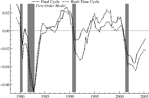
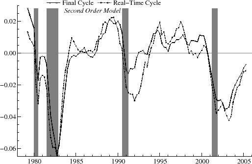
Examples are shown in figures 13, 14, and 15 for and 4. The real-time and final cycles track each other fairly well over much of the sample period. The cycles tend to be close in the early phase of recessions. In the case of the 1990-1 recession, it appears that the downturn in the real-time cycle leads the decline in the final cycle by a slight margin. The biggest discrepancy in the cycles occurs in the period following the 1990-1 recession, where the real-time cycle appears to overestimate the extent of the fall in output and then makes a late call in marking the start of the upturn. On the other hand, the magnitude of this discrepancy dimishes for larger , as seen from inspection of the graphs or from inspection of the measure in table 8. Overall, there are several stretches where the real-time and final estimates show the same timing and kinds of transitions, even though their values may differ. For instance, in the recovery after the 1981-2 recession, there is a good deal of accuracy in timing the turning point, even though the level of the real-time estimate soon departs from that of the final estimate as the real-time estimate accelerates upward more quickly.

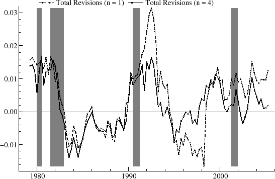
Figure 16 shows the revisions series for both and 4. The series follow each other closely at certain times, for instance, 1986 to 1990, but at other times, the revisions are clearly more favorable. Especially noticeable is the period 1991 to 1993, where the graph shows the revisions for reaching about twice the value for . Between 1996 and 1998, and between 2000 and 2002, the series for is clearly smaller in magnitude. This improved performance may be due to the combination of having more noise removed from the signal (output gap), as well as linking the "cleaner" signals in the two series through the assumption of correlated components.

5 Conclusions

This paper has investigated real-time estimation of the output gap using models based on the class of stochastic cycles introduced in Harvey and Trimbur (2003). In a univariate analysis, the models give estimates whose properties are comparable to those of the methods examined in Orphanides and van Norden (2002). This analysis demonstrates the viability of using model-based band-pass filters in real-time. Overall, the higher order models performed better than the basic (first order) model in term of fit and accuracy measures.

The real-time estimates tend to perform well around the NBER-dated recessions, particularly for higher orders, and appear to gauge turning points relatively well. This suggests that, even though discrepancies remain between real-time and final estimates throughout the sample period, during periods of transition, the direction of the real-time estimates can serve as a valuable guide.

Throughout the paper, a few references to Bayesian methods have been made. Given the irregularities in the likelihood surface, in some cases, I have used the convention of fixing the central period to a value plausible for business cycle fluctuations. A more satisfactory way to express business cycle expectations is to set up a Bayesian prior, as in Harvey, Trimbur, and van Dijk (2007), and using the Bayesian approach allows for other advantages, such as accounting for parameter uncertainty. A possible topic for future work would be to explore the feasibility of Bayesian estimation in real-time to see if consistent use of prior knowledge may perhaps lead to further improvements in the quality of real-time estimates of the output gap.

In this paper, I have focussed on a classical approach and have shown how the pooling of information from a closely related series can increase the accuracy of real-time estimation and improve revision properties. The capacity utilization series has clear cyclical dynamics, and I have demonstrated the relatively small revisions to the cycle as new data become available. It seems natural to link the output gap with CU given its definition as a measure of deviation from potential. This relationship has been expressed in a bivariate unobserved components model in which the cycles in CU and real GDP are intertwined. Indeed, the estimated correlation parameter between the two cycles, which rises with increasing order, reaches 0.92 for . The properties of revisions and accuracy of real-time estimates are significantly improved relative to the univariate analysis, and again, the higher order models outperform the basic model. The correlation between real-time and final estimates of the GDP gap peaks at about 0.93 for .

References

Basistha A, Startz R. 2007. Measuring the NAIRU with Reduced Uncertainty: a Multiple Indicator-Common Cycle Approach. Review of Economics and Statistics, forthcoming.

Baxter M, King R. 1999. Measuring business cycles: approximate band-pass filters for economic time series. Review of Economics and Statistics81 : 575-93.

Carvalho V, Harvey A, and Trimbur T. 2007. A note on common cycles, common trends and convergence. Journal of Business and Economic Statistics 68 : 863-77.

Christiano L, Fitzgerald T. 2003. The band pass filter. International Economic Review 44 : 435-65.

Corrado C, Mattey J. 1997. Capacity Utilization. Journal of Economic Perspectives 11 : 151-167.

Croushore D, Stark T. 2001. A Real-Time Data Set for Macroeconomists. Journal of Econometrics 105 : 111-130.

Doornik J. 2006. Ox: An Object-Oriented Matrix Programming Language. Timberlake Consultants Ltd.: London.

Durbin J, Koopman S. 2001. Time series analysis by state space methods. Oxford University Press: Oxford.

Harvey A. Forecasting, structural time series models and the Kalman filter. Cambridge University Press: Cambridge.

Harvey A, Koopman S. 1997. Multivariate structural time series models. In System dynamics in economic and financial models, Heij C et al(eds). Wiley and Sons: Chichester.

Harvey A, Trimbur T. 2003. General model-based filters for extracting trends and cycles in economic time series. Review of Economics and Statistics 85 : 244-55.

Harvey A, Trimbur T, van Dijk H. 2007. Trends and cycles in economic time series: a Bayesian approach. Journal of Econometrics 140 : 618-649.

Koopman S, Shephard N, Doornik J. 1999. Statistical algorithms for models in state space using SsfPack 2.2. Econometrics Journal2 : 113-66.

Kuttner K. 1994. Estimating potential output as a latent variable. Journal of Business and Economic Statistics 12 : 361-8.

Morin N, Stevens J. 2005. Estimating Capacity Utilization from Survey Data. IFC Bulletin 20 : 42-61.

Murray C. 2002. Cyclical properties of Baxter-King filtered time series. Review of Economics and Statistics, 85 : 471-6.

Orphanides A, Van Norden S. 2002. The unreliability of output gap estimates in real-time. Review of Economics and Statistics 84 : 569-83.

Planas C, Rossi A. 2004. Can inflation data improve the real-time reliability of output gap estimates? Journal of Applied Econometrics 19: 121-33.

Trimbur T. 2006. Properties of higher order stochastic cycles. Journal of Time Series Analysis 27 : 1-17.

Watson M. 2007. How Accurate are Real-Time Estimates of Output Trends and Gaps? Federal Reserve Bank of Richmond Economic Quarterly 93 : 143-61.

**Figure 1:** Most recent vintage (August 2007) for capacity utilization, sample period January 1969 to July 2007.

**Figure 2:** Estimated second order cycle in capacity utilization for January 1969 to July 2007 (August 2007 vintage).

**Figure 3:** Estimated irregular component in capacity utilization for January 1969 to July 2007 (August 2007 vintage).

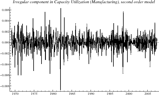Table 1.--Estimates for cyclical model of monthly capacity utilization

	$\overline{\mu}$	$\sigma_{\psi}^{2}$ $\times10^{3}$	$\sigma_{\varepsilon}^{2}$ $\times10^{5}$	$\rho$	2 $\pi/\lambda_{c}$	$R_{D}^{2}$	$\widehat{\sigma}$
1	0.7995	1.48	0.00	0.988	85.32	0.12	6.08	65.6	-3396.4
2	0.8003	1.37	0.72	0.868	--	0.17	5.91	32.7	-3423.4
3	0.8001	1.21	0.92	0.761	--	0.13	6.03	44.3	-3404.2
4	0.8000	1.16	1.00	0.685	--	0.11	6.11	52.4	-3392.5
5	0.8000	1.13	1.04	0.627	--	0.10	6.16	57.6	-3385.3
6	0.7999	1.11	1.06	0.581	--	0.09	6.19	61.2	-3380.4

Note: Results for August 2007 vintage (sample period January 1969 to July 2007). For ${\small n>1},$ the cycle period, 2 ${\small\pi /\lambda}_{{\small c}},$ was set equal to the value obtained for ${\small n=1}.$ $\overline{{\small\mu}}$ (level) $,{\small\sigma }_{\varepsilon}^{2}$ (the irregular variance), and ${\small\rho}%$ correspond to other parameters in model (1). ${\small\sigma}_{\psi}^{2}$ is the cycle variance. The designation ` ${\small\times10}^{3}$ ' in the second row means that the variance parameter has been multiplied by ${\small 10}^{3}.$

**Figure 4:** The first available vintage (August 1979) for capacity utilization, sample period January 1969 to July 1979.

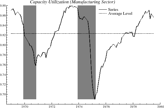Table 2.--Estimates for cyclical model of monthly capacity utilization

	$\overline{\mu}$	$\sigma_{\psi}^{2}$ $\times10^{3}$	$\sigma_{\varepsilon}^{2}$ $\times10^{5}$	$\rho$	2 $\pi/\lambda_{c}$	$R_{D}^{2}$	$\widehat{\sigma}$ $\times10^{3}$	Q(P)	AIC
1	0.8179	1.75	0	0.984	49.39	0.279	7.79	56.6	-858.4
2	0.8234	1.86	0.40	0.829	83.47	0.398	7.11	10.9	-881.6
3	0.8226	1.59	0.81	0.705	--	0.383	7.24	16.4	-877.0
4	0.8224	1.48	0.97	0.618	--	0.363	7.37	22.7	-872.7
5	0.8224	1.44	1.10	0.561	--	0.347	7.46	28.6	-869.6
6	0.8225	1.47	1.27	0.534	--	0.335	7.52	34.5	-867.5

Note: Results for August 1979 vintage (sample period January 1969 to July 1979). For ${\small n>2},$ the cycle period, 2 ${\small\pi /\lambda}_{{\small c}},$ was set equal to the average of the periods for ${\small n=1}$ and 2. See also Note for Table 1.

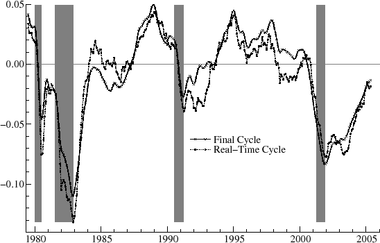**Figure 5:** Final and real-time cyclical estimates for capacity utilization for July 1979 to May 2005 for model. The latest vintage is August 2007.

Table 3.-- Properties of Revisions: Monthly Capacity Utilization

	$\times10^{3}$
1	4.76	0.0126	0.0134	0.0347	-0.0276	0.943
2	4.90	0.0123	0.0133	0.0315	-0.0237	0.951
3	4.78	0.0124	0.0133	0.0333	-0.0235	0.950
4	4.76	0.0125	0.0134	0.0342	-0.0236	0.949
5	4.76	0.0125	0.0134	0.0347	-0.0237	0.949
6	4.77	0.0125	0.0134	0.0348	-0.0237	0.948

Note: The integer ${\small n}$ denotes the order of the cyclical model. ${\small Mean}$ is the average revision, while ${\small Std}$ denotes the standard deviation of revisions. ${\small RMSE}$ is the root mean-square of revisions. ${\small Max}$ stands for the maximum revision, ${\small Min}$ for the minimum revision. ${\small ACF(1)}$ is the first order serial correlation in the revision series.

**Figure 6:** Revisions in cyclical estimates for capacity utilization for July 1979 to May 2005 for and models.

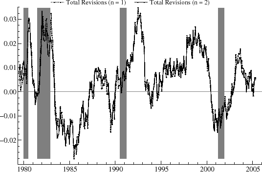Table 4.-- Real-Time Accuracy: Monthly Capacity Utilization


1	0.946	0.345	0.818
2	0.945	0.335	0.829
3	0.944	0.338	0.817
4	0.943	0.340	0.813
5	0.944	0.340	0.814
6	0.943	0.341	0.814

Note: ${\small Corr}$ stands for the correlation between real-time and final estimates. ${\small NS}$ is the ratio of the standard deviation of revisions to the standard deviation of the final output gap estimates. ${\small CoSign}$ gives the frequency with which the final and real-time estimates have the same sign.

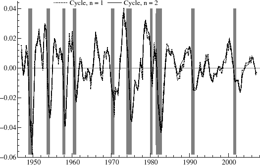**Figure 7:** Series of quarterly US real GDP (logarithms), with estimated trend, for the vintage of 2007Q3 (sample period from 1947Q1 to 2007Q2) with .

**Figure 8:** Estimated cycles (first and second order) in US real GDP (logarithms) shown for the vintage of 2007Q3 (sample period from 1947Q1 to 2007Q2).

Table 5.--Estimates for cyclical model of quarterly real GDP

	$\sigma_{\zeta}^{2}$ $\times10^{6}$	$\sigma_{\psi}^{2}$ $\times10^{4}$	$\sigma_{\varepsilon}^{2}$ $\times10^{5}$	$\rho$	2 $\pi/\lambda_{c}$	$R_{D}^{2}$	$\widehat{\sigma}$ $\times10^{3}$
1	1.52	2.78	0	0.897	18.36	0.054	9.54	30.9	-1536.6
2	1.17	3.12	1.24	0.716	--	0.083	9.39	16.9	-1543.8
3	1.19	3.05	1.56	0.602	--	0.081	9.40	17.3	-1543.3
4	1.23	2.98	1.66	0.521	--	0.078	9.42	18.0	-1542.5
5	1.28	2.91	1.71	0.461	--	0.075	9.43	18.6	-1541.9
6	1.30	2.87	1.73	0.415	--	0.074	9.44	19.0	-1541.4

Note: Results for 2007Q3 vintage (sample period 1947Q1 to 2007Q2). $\sigma_{\zeta}^{2}$ denotes the slope disturbance variance parameter in model (3). See note under table 1 for descriptions of other parameters.

Table 6.--Estimates for cyclical model of real GDP

	$\sigma_{\zeta}^{2}$ $\times10^{6}$	$\sigma_{\psi}^{2}$ $\times10^{4}$	$\sigma_{\varepsilon}^{2}$ $\times10^{5}$	$\rho$	2 $\pi/\lambda_{c}$	$R_{D}^{2}$	$\widehat{\sigma}$ $\times10^{3}$	Q(P)	AIC
1	1.21	4.02	0	0.918	17.47	0.128	10.28	10.85	-792.43
2	0.859	5.07	1.25	0.726	21.52	0.156	10.11	7.18	-796.80
3	0.933	4.71	1.51	0.622	--	0.160	10.09	7.82	-797.29
4	0.928	4.71	1.86	0.547	--	0.161	10.09	8.16	-797.46
5	0.925	4.70	1.91	0.490	--	0.162	10.08	8.32	-797.53
6	0.925	4.69	1.94	0.446	--	0.162	10.08	8.41	-797.58

Note: Results for 1979Q3 vintage (sample period 1947Q1 to 1979Q2). For ${\small n>2},$ the cycle period, 2 $\pi/\lambda_{c},$ was set equal to the average of the periods for and 2. See notes to tables 1 and 5 for further explanation.

Table 7.--Properties of Revisions: Real GDP

	$\times10^{4}$
1	5.7	0.01258	0.01260	0.0371	-0.0251	0.865
2	-0.6	0.01212	0.01213	0.0271	-0.0307	0.915
3	-1.4	0.01206	0.01206	0.0284	-0.0320	0.911
4	-1.8	0.01185	0.01185	0.0284	-0.0322	0.907
5	-1.5	0.01169	0.01169	0.0283	-0.0323	0.905
6	-1.4	0.01151	0.01151	0.0281	-0.0321	0.902

Note: See note under table 3.

Table 8.--Real-Time Accuracy: Real GDP

			CoSign
1	0.474	1.089	0.601
2	0.518	0.891	0.638
3	0.501	0.897	0.628
4	0.494	0.901	0.609
5	0.492	0.901	0.609
6	0.493	0.902	0.600

Note: See note under table 4.

**Figure 9:** Real-time and final estimates of the output gap from 1979Q2 to 2005Q2, for cyclical model with .

**Figure 10:** Real-time and final estimates of the output gap from 1979Q2 to 2005Q2, for cyclical model with .

**Figure 11:** Revisions of output gap estimates, sample period 1979Q2 to 2005Q2, for cyclical model with and . (Vintages from 1979Q3 to 2007Q3)

**Figure 12:** Estimated cycles (first and fourth order) in US real GDP (logarithms) shown for the vintage of 2007Q3 (sample period from 1947Q1 to 2007Q2) for bivariate model with capacity utilization.

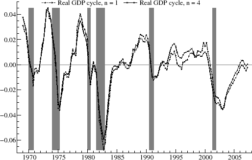Table 9a.--Estimates for bivariate cyclical model: capacity utilization

	$\overline{\mu}$	$\sigma_{\psi}^{2}$ $\times10^{3}$	$\sigma_{\varepsilon}^{2}$ $\times10^{5}$	$R_{D}^{2}$	$\widehat{\sigma}$
1	0.800	1.15	0	0.212	0.0119	41.58
2	0.800	1.43	0.03	0.344	0.0108	36.98
3	0.799	1.29	0.34	0.319	0.0110	42.12
4	0.798	1.22	1.26	0.297	0.0112	54.85
5	0.797	1.18	1.84	0.293	0.0112	59.75
6	0.797	1.17	2.12	0.287	0.0113	62.42

Note: Results for 2007Q3 vintage (sample period 1969Q1 to 2007Q2). See note under table 1.

Table 9b.--Estimates for bivariate cyclical model: Real GDP

	$\sigma_{\zeta}^{2}$ $\times10^{7}$	$\sigma_{\psi}^{2}$ $\times10^{4}$	$\sigma_{\varepsilon}^{2}$ $\times10^{5}$	$R_{D}^{2}$	$\widehat{\sigma}$ $\times10^{3}$
1	3.21	3.57	0.55	0.098	7.83	24.43
2	4.29	3.52	1.01	0.154	7.58	15.03
3	5.57	3.10	1.09	0.137	7.65	16.11
4	5.77	3.01	1.29	0.133	7.68	17.10
5	5.77	2.96	1.41	0.135	7.66	18.63
6	5.83	2.97	1.48	0.134	7.67	19.44

Note: Results for 2007Q3 vintage (sample period 1969Q1 to 2007Q2). See note under table 5.

Table 9c.--Estimates for bivariate cyclical model

	$\nu_{\kappa}$	$\nu_{\varepsilon}$	$\rho$	2 $\pi/\lambda_{c}$	AIC
1	0.780	0.742	0.945	30.3	-2023.6
2	0.891	0.525	0.725	--	-2056.4
3	0.918	0.342	0.551	--	-2049.2
4	0.919	0.454	0.479	--	-2042.2
5	0.918	0.505	0.436	--	-2039.1
6	0.920	0.524	0.400	--	-2035.4

Note: Results for 2007Q3 vintage (sample period 1969Q1 to 2007Q2). See note under table 1. $\nu_{\kappa}$ is the correlation between cyclical disturbances in real GDP and CU, and $\nu_{\varepsilon}%$ is the correlation between irregular components in real GDP and CU.

**Figure 13:** Real-time versus final estimates of the GDP gap, 1979Q3 to 2005Q2 for bivariate cyclical model with .

**Figure 14:** Real-time versus final estimates of the GDP gap, 1979Q3 to 2005Q2 for bivariate cyclical model with .

**Figure 15:** Real-time versus final estimates of the GDP gap, 1979Q3 to 2005Q2 for bivariate cyclical model with .

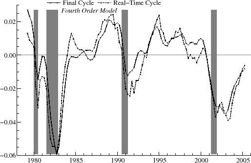Table 10.--Properties of Revisions for bivariate model: Real GDP

	$\times10^{3}$
1	3.89	0.01056	0.01124	0.0313	-0.0164	0.913
2	3.59	0.00825	0.00901	0.0256	-0.0118	0.915
3	2.51	0.00757	0.00797	0.0191	-0.0127	0.904
4	2.11	0.00746	0.00776	0.0168	-0.0138	0.879
5	1.62	0.00760	0.00777	0.0184	-0.0150	0.843
6	1.18	0.00749	0.00758	0.0209	-0.0156	0.838

Note: See Note for Table 3.

Table 11.--Real-Time Accuracy for bivariate model: Real GDP

			CoSign
1	0.890	0.546	0.838
2	0.918	0.445	0.829
3	0.928	0.417	0.791
4	0.925	0.410	0.800
5	0.922	0.415	0.809
6	0.920	0.408	0.810

Note: See Note for Table 4.

**Figure 16:** Revisions of output gap estimates, sample period 1979Q2 to 2005Q2, for bivariate cyclical model with and . (Vintages from 1979Q3 to 2007Q3)

Footnotes

* Address: Division of Research and Statistics; 20th and C Street, NW - Stop 82; Federal Reserve Board; Washington DC 20551. Telephone: (202) 452 2935. Fax: (202) 736 1937. Email:[email protected]. Return to Text

1. The dates of expansions and recessions are established by the NBER; note that this classification is based on judgmental procedures applied with hindsight. Further, there may be loss of information in moving from continuous-valued cyclical components to a binary upturn-downturn labelling. Return to Text

2. The model structure in (2) has a degree of symmetry in that $\psi_{n,t}$ and $\psi_{n,t}^{\ast}$ are both subject to shocks, and similarly there is balance in the equations for [ $\psi_{i,t}%$ , $\psi_{i,t}^{\ast}$ ] in the recursion when both $\psi_{i-1,t-1}$ and $\psi_{i-1,t-1}^{\ast}$ enter on the right side. An alternative form, called the Butterworth form, has both $\kappa_{t}^{\ast}$ and $\psi_{i-1,t-1}^{\ast}$ replaced by zero and $\psi_{i-1,t-1}$ shifted ahead to $\psi_{i-1,t}$ ; this gives a more direct link with the frequency domain.

In what follows, I work with this balanced form. Experience suggests that the balanced form works slightly better empirically for US macreconomic series and produces more plausible periods. A further advantage of (2) is that the time-domain properties of the stochastic cycle are more easily derived compared to the Butterworth form. Return to Text

3. Analytical expressions for the variance in terms of

, $\sigma_{\kappa}^{2}$ , and $\rho$ are given in Trimbur (2006). Return to Text

4. Harvey and Trimbur (2003) introduce a class of model-based band-pass filters based on the slight variation of (2) called the Butterworth form. The

th order cycle then gives rise to a generalized band-pass Butterworth filter of order

. This encompasses a wide array of patterns for the gain; as

increases, for instance, the equivalent of the `ideal' filter is obtained as a special case. Return to Text

5. In particular, higher

are associated with sharper band pass filters in the frequency domain. The location of the left and right boundaries and the particular shape might, however, be different. For instance, it is shown in Harvey and Trimbur (2003) that for US investment, the results of applying the optimal band-pass filter for

differed from the results of applying the BK filter. Return to Text

6. Note that since the analysis in Watson (2006) is based on the Baxter-King filter (augmented with endpoint adjustments), the results are subject to the same criticism of possible distortions when using the "ideal" filter that were noted previously. Return to Text

^♣ This version is optimized for use by screen readers. Descriptions for all mathematical expressions are provided in LaTex format. A printable pdf version is available. Return to Text