
Using Policy Intervention to Identify Financial Stress1
Keywords: Financial stress, financial markets, financial institutions
Abstract:
This paper describes the construction of a financial stress index. This stress index differs from other indexes in that it incorporates the co-movement and volatility of financial series as well as the levels of the series. Our index also uses past experience more than others to guide the assessment about which characteristics of the data suggest financial stress exists. In addition to describing the construction of our financial stress index, we spend some time discussing issues relevant to the general construction of stress indexes.
1 Introduction
The purpose of this paper is two-fold. First, we describe the construction of a financial stress index. There have been a number of such indexes introduced in the past few years, see for instance Brave and Butters (2011), Hakkio and Keeton (2009), Illing and Liu (2006), Kliesen and Smith (2010), Kritzman, Li, Page, and Rigobon (2010), Oet, Eiben, and Bianco (2011), and Bank of America Merrill Lynch (2010). Nevertheless, the measure discussed here has some novel features which make it a useful addition to the literature. The second purpose of this paper is to provide a more detailed discussion of some of the issues regarding how financial stress indexes are constructed.5
The stress index described in this paper builds on the index introduced by Nelson and Perli (2005). That index is based on the behavior of 12 financial series that in turn capture market measures of risk pricing, uncertainty, and liquidity. To construct their overall index, Nelson and Perli first calculate three sub-indexes based on the level, speed of change, and co-movement of the series. They then select historical crisis periods and, using a logistic regression framwork, examine whether the three sub-indexes are associated with being in a crisis period or a normal period. The results of the logit regression are used to convert the sub-indexes into an overall stress index.
The stress index described here follows the same general procedure used by Nelson and Perli, but make some adjustments. The most substantive change is the way crisis periods are selected. Nelson and Perli choose crisis periods based on opinion regarding when financial markets were under stress, a method similar to Illing and Liu (2006). In this paper, we base crisis periods on whether policymakers responsible for regulating financial institutions intervened in financial markets out of concern about systemic risks posed by troubles at a U.S. financial institution or impaired functioning in a U.S. financial market. As such, the financial stress index presented in this paper can be interpreted as indicating the degree to which conditions in financial markets are similar to periods when policymakers were concerned enough about systemic risks to intervene. While this procedural shift does not have much practical impact on the resulting index, it does mark a consequential shift in interpretation. We make a few other changes to the index described by Nelson and Perli, such as using a volatility sub-index rather than a rate of change sub-index and modifing the composition of the 12 underlying financial series. All these changes are noted below.
The structure of the stress index presented here differs somewhat from other stress indexes described in the literature and is a useful vehicle for discussing some issues related to the construction of the stress indexes. The first issue we consider is the role of a financial stress index versus a financial conditions index. A financial conditions index provides some information on the price or non-price costs of obtaining credit. A financial stress index provides more information on whether markets are functioning or behaving in a typical fashion. Both issues are important yet quite different; it is necessary to consider what a particular index is capturing to determine which should be applied in a particular setting.
The second issue is which characteristics of asset prices matter. Many stress indexes focus on levels of different variables, whereas the measure described here incorporates multiple dimensions. We argue that behavioral differences in markets that reflect different levels of stress indicate that looking at more than just the level is useful.
The third issue follows from the second. When more than one financial series is used, those series need to be combined in some fashion. While a variety of weighting mechanisms have been employed, principal-component based approaches and market-size weighting schemes have been the most common. The approach here draws more heavily on historical experience to determine appropriate weights.
The fourth issue is the use of historical experience to develop the stress index. Many stress indexes do this to some extent by using history as guide for looking at which financial series to use in the construction of the index. The measure in this paper involves greater use of the historical experience. We use historical crisis episodes and policymaker responses to financial market stresses to gauge the importance of our sub-indexes in the construction of an overall metric of stress.
Related to the use of history as a guide is the role of updating, our fifth issue. As more time passes and the underlying series used to construct the stress index have either more placid periods or more volatile periods, one might re-interpret history. In particular, periods that might have looked stressful prior to the experience of the fall of 2008 may no longer look particularly problematic. The issue of updating impacts all financial stress indexes, but may have a larger impact on the index described here given the procedure that is used.
The paper is organized as follows. In section two, we describe the construction of the financial stress index. In section three, we discuss each of the issues noted here and compare our approach to other stress indexes. Section four concludes.
2 Development of the Financial Stress Index
As in Nelson and Perli (2005), the financial stress index described here is a composite of three sub-indexes, each of which in turn describes a specific aggregate characteristic of twelve underlying data series. Here, we present the basic building blocks and review the steps taken to convert these into an overall stress index. The underlying data consist of twelve financial series that cover market liquidity, risk pricing, and uncertainty.6 All of these series would be expected to respond to financial stress.7 To make the series comparable, we standardize each variable. We examine the data at a daily frequency using the 5-day moving average of each variable to reduce noise.8
2.1 The Levels Sub-index
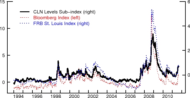 |
In most measures of financial market stress or strain, the focus is squarely on the level of various financial market indicators, which is captured here in the first sub-index. This sub-index is simply the average of the twelve standardized series, plotted as the black line in Figure 1. The series are standardized such that each value is the number of standard deviations that variable's level is away from its long-run mean. As might be expected, the series is higher during periods often considered to be stressful, such as the one around the Russian default/collapse of Long Term Capital Management (LTCM) in late 1998 or during the recent financial crisis period from 2007-2009.
In constructing any one of the other recent stress indexes, authors have used many different variables as well as several different aggregation strategies. The index here uses a fairly small number of variables and a basic aggregation methodology for reasons of relative parsimony. We argue that this simple average provides the majority of the information regarding the level of the various series, and that these series capture the majority of the distinct movements associated with financial stress. Some other financial stress indexes have used more complex aggregation methods, for example principal components, rather than the average to combine series. Doing so here would have little material effect. Similarly, some indexes use many more variables in their effort to characterize financial stress. As shown in Figure 1, two other stress indexes that use more variables and different aggregation methods yield largely similar results. Our point is not that our choice of variables or simple averaging approach is superior, rather that there appears to be something of a consensus regarding measures of the aggregate level of financial market variables and that our first sub-index yields the results found by other researchers and organizations.
2.2 The Volatility Sub-Index
Not only do the levels of measures of risk, uncertainty, and liquidity premia tend to increase, during periods of financial stress, their volaility increases as well. Typically, during the onset of a crisis, prices of risky or illiquid assets plunge, which causes risk spreads and liquidity spreads to widen sharply. Other scholars, such as Kritzman, Li, Page, and Rigobon (2010) have noted that the prices of risk assets remains especially sensitive to news as the crisis continues. This idea motivates the construction of the second sub-index, a volatility sub-index, shown in figure 2.9 This sub-index is again an average across the twelve underlying financial variables, this time looking at the sum of squared daily changes over an 8-week rolling window.10 Changes in volatility are expected to correspond to shifts between more stressful and less stressful periods.
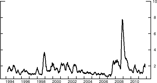 |
Our measure of realized volatility allows us to assess changes in asset price volatility that may not be as forward-looking as changes in implied volatility exercises, but give us the ability to look further back in time than options-based metrics would. The series in Figure 2 demonstrates changes in volatility during several peak stress events, most notably in the time immediately following the Lehman Brothers failure in late 2008.
2.3 The Comovement Sub-Index
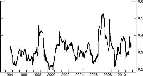
Finally, during financial stress episodes, asset prices tend to move together more; "the correlation goes to one" in colloquial terms. The third sub-index looks at the time-varying level of comovement among the variables. To capture the changing co-movement, we again follow Nelson and Perli (2005) and calculate the principal components of the changes in the twelve series using 26-week rolling windows. The comovement sub-index is the percent of total variation explained by the first principal component in each 26-week window. The higher this measure, the more of the changes in the underlying series can be explained by a single common factor. This sub-index is plotted in Figure 3.
The data in Figure 3 show that the percentage of variation explained by a single common factor was also at its peak during the financial crisis of 2007-2009, but that the events of 2007-2009 were less of an outlier than was the case in the other sub-indexes.
2.4 Historical Stress Episodes
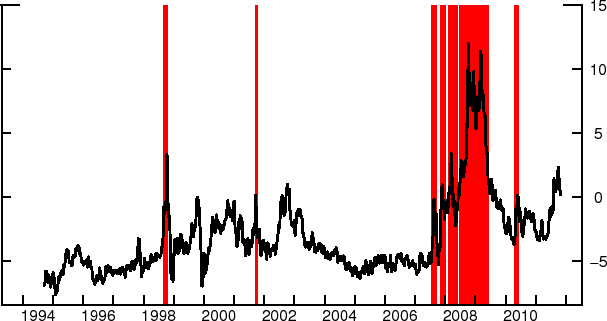
To combine the three sub-indexes into a single index, it is useful to consider how they behaved during historical stress episodes. To determine what constituted a stress event, we start by identifying interventions by policymakers that occurred out of concern that troubles at a U.S. financial institution or the impairment in functioning of a U.S. financial market might present systemic risks to financial stability and have negative consequences for economic activity. The policymakers we look at include the Federal Reserve, the Federal Deposit Insurance Corporation, and the Treasury Department; although, in the final analysis, interventions by the Federal Reserve end up being far more common than those of other agencies. The types of interventions that qualify are fairly broad, as our rule is to include all actions taken by policymakers that are done specifically to protect financial market functioning. For example, the action by the Federal Reserve to convene a conference of the heads of major financial firms to organize the rescue of Long Term Capital Management counts as an intervention, as does the extraordinary provision of liquidity by the Federal Reserve on and in the days following September 11, 2001, and of course the facilities of the three agencies designed to confront the market functioning concerns of 2007-2009. We count as an intervention the announcement of any new action, or any escalation of previous interventions, but we do not count the implementation of a given action.11 The complete list of interventions is provided in Appendix B. We do not consider changes in monetary policy to be interventions, as the motivating factor for that action is considered to be more macroeconomic, and less in consideration of financial market functioning, per se.12
We consider the stress episodes to be the periods extending from four weeks before an intervention is announced to four weeks after this announcement.13 This time frame is meant to capture the majority of the period in which the stress built to a level that resulted in policymaker action, as well as a period following the action that encompassed evaluation of the market reaction, and a lag for implementation of the policy. A sensitivity analysis of the choice of window size demonstrates that the size of the total window around the policy announcement date only becomes a significant factor if it is shrunk down to 4 weeks or below. Windows of 5-16 weeks produce similar results, so a choice was made to remain on the smaller end of the spectrum to avoid false positives.
Some of the interventions we consider are ones that occur on a single day, such as the August 10, 2007 issuance of a statement reaffirming the commitment to provide liquidity and the addition of an extraordinary amount of reserves through multiple operations, while other interventions resulted in facilities that were in use for some time, such as the Term Auction Facility. In both cases, we look only at the four weeks surrounding the annoucement. By looking at the eight-week window, even in cases in which the annoucement concerned the creation of a facility that would be in place for some time, we focus on conditions that prevailed in financial markets around the time that the policymakers decided to intervene. We also avoid confounding, at least to some extent, the conditions in financial markets leading to the intervention and the impact on financial markets from the announced intervention.
We treat periods outside those policy intervention windows as "normal." In order to follow our rule for determining stress period, we do not classify the last 4 weeks of the data as either a stress period or a normal period; this is explained further in Section 3.5. The twelve underlying series are all available consistently since January of 1994. Given the rolling window structure of the data, all three sub-indexes become available starting in July of 1994. The last observation used here is from October 31, 2011.
2.5 Logistic Regression Model
To look at how the sub-indexes behaved in the stress periods, we use a logistic regression framework and regress a stress episode indicator on our three sub-indexes, levels (![]() ), changes in
volatility (
), changes in
volatility (![]() ), and comovement (
), and comovement (![]() ). The regression takes the form:
). The regression takes the form:
The results appear in Table 1. Higher levels of all three of the sub-indexes are associated with being in a stress period. It is notable that, despite the common spike across each of the three sub-indexes in the financial crisis of 2007-2009, each of these sub-indexes remains statistically and economically important in helping us to define an overall index of financial stress. After taking account of the different variances in the sub-indexes, changes in the sub-index capturing the co-movement of the different variables appears most strongly associated with the shift from a normal to a stress period, while the sub-index capturing the change in asset market volatility has the smallest, though still strongly significant, relative impact in determining a stress period.
Table 1: Logistic regression model estimation results
| Estimate | Std. Error |
|
||
| Intercept | -9.6003 | 0.5280 | -18.184 |
|
| L | 6.5802 | 0.3400 | 19.354 |
|
| V | -1.5883 | 0.2043 | -7.773 |
|
| C | 23.6309 | 1.4409 | 16.400 |
|
2.6 Index Construction
We can use the coefficients from the logistic regression in equation (2.1) in at least one of two ways. The first method would be to simply use the coefficients as weights to combine the three sub-indexes that describe the three characteristics of the data we feel help to describe financial stress:
This version of the index is shown in Figure 4.14
 |
As we use a logistic regression framework to derive the coefficients it is also natural to express the financial index as the estimated probability of being in a period of stress. This estimated probability is given as:
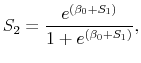
and is shown in Figure 5.
2.7 Interpreting the output
To be clear, the sense in which this index is expressing a probability is limited to the context of identifying current conditions. The probability in Figure 5 is the probability that financial markets are currently experiencing conditions identical to those identified as stress episodes.
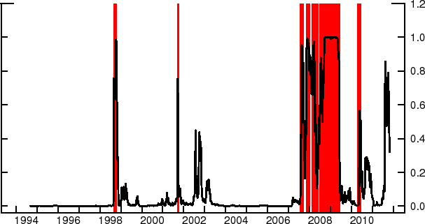 |
Of course, policymakers have access to the information entering the analysis in real time anyway, so they would likely know if there was a financial crisis or not. What this index provides is a sense of historical context for those opinions. Rather than thinking of this as a probability of stress episode, one should think of it as a statistical measure of the similarity between current conditions, and those that prevailed at a time already identified as a crisis. The more continuous measure in Figure 4 is simply a smoother interpretation of the same information, which is useful to researchers in need of a more continuous series to study effects of stress on other areas of the macroeconomy.
We emphasize that the stress index presented here is descriptive of financial conditions and is not designed as an early warning system. Specifically it does not provide an indication of the likelihood of a financial crisis over any particular time horizon.
3.1 Financial Stress versus Financial Condition
A financial stress index (FSI) is meant to capture something about the functioning or fragility of financial markets.15 Impaired functioning might take the form of increased difficulty in executing transactions or an inability of intermediaries to fund their market-making operations at usual tenors. Fragility might take the form of exceptionally heightened sensitivity to new information or shocks (as in Kritzman, Li, Page, and Rigobon (2010)). Hakkio and Keeton (2009) note that financial stress tends to be associated with increased uncertainty about the fundamental value of assets, increased uncertainty about the behavior of other investors, increased asymmetry of information, flights to quality, and flights to liquidity; all of these items would reduce functioning in markets and might result in market dislocations. A financial stress index is a device to distill the information about financial market functioning and fragility.
Having a measure of the stress in financial markets and being able to identify difficulties early can enhance policymakers' ability to take steps to alleviate the crisis (IMF 2009). In this regard, our index might be particularly apt as it provides a comparison of current conditions to periods when policymakers opted to intervene out of concern regarding financial stability.
A financial conditions index (FCI), by contrast, is more useful in assessing the macroeconomic implications of developments in the financial sector (see English, Tsatsaronis, and Zoli (2005)). Information about such things as the cost of borrowing for households, cost of capital for business, real exchange rates, and household wealth, has implications for spending, investment, output, and inflation. An FCI extracts information from a wide variety of indicators about these items and condenses it into a single measure. One way to construct an FCI is to extract one or more principal components from a large number of financial series that reflect items such as borrowing costs and wealth. Researchers sometimes adjust the underlying financial series to remove the impact of lagged real economic conditions prior to the principal component computation. By contructing the FCIs in this way, it is hoped that they provide an indication about some financial conditions that cannot be measured directly, such as risk aversion and sentiment. As shown by English, Tsatsaronis, and Zoli (2005) and Hatzius, Hooper, Mishkin, Schoenholtz, and Watson (2010), FCIs can be useful in forecasting economic activity. Thus, such indexes are also useful for policymakers, but more in connection with setting monetary (or fiscal) policy.
FSIs and FCIs serve quite different purposes; however, such distinctions are not always clear in the literature.16 Clouding the issue, FSIs and FCIs may be constructed in similar ways and may include some similar indicators. For example, a number of such indicies are constructed using principal component analysis. The spread between yields on corporate bonds and Treasury bonds serves as a measure of risk and the cost of financing and is often included in both FSIs and FCIs. However, as noted above, other items can differ. FCIs often include other measures of the cost of funding, such as indicators of lending standards, or measures of household wealth. FSIs often include some measures of liquidity in financial markets and of uncertainty. It is important for the creators and users of these FSIs and FCIs to be careful in considering how they are constructed and what they measure to effectively use and interpret them. In constructing the index in this paper, we have tried to select underlying series that reflect the functioning and fragility of markets and relate developments in these measures to stress episodes; thus we consider our index to be clearly tied to financial stress.
3.2 Dimensions of asset price developments
Many financial stress indexes focus on the level of variables such as risk spreads, spreads that are indicative of liquidity premia, and indicators of the level of uncertainty such as measures of implied volatility. These factors certainly matter and they are included here as well.
However, as noted above, asset prices are often described as displaying additional characteristics during financial crises. A stress episode is often characterized by rapid changes in asset prices. Hakkio and Keeton (2009) argue that greater volatility in the market prices of the assets reflects the heightened uncertainty about fundamental values that generally accompanies financial stress. News and economic shocks can thus result in large reactions in asset prices. Often episodes of financial stress are associated with an initial sharp plunge in asset prices, but large movements in asset prices may continue as long as strains in markets persist. The sub-index based on the volatility of asset prices is meant to capture this dynamic of financial stress. As indicated by the logit analysis in Table 1, this measure of asset price movements is indeed generally associated with periods considered to be stressful.
Another characteristic of financial stress periods is that asset prices tend to move more together. The increased co-movement may reflect heightened concerns about macroeconomic or other broad factors that will impact a wide range of asset prices. The IMF (2009) suggests that tail risk dependence can boost co-movement and be a measure of systemic risk. Heightened co-movement could also be related to more microeconomic issues such as increased use of quantitative risk models that are similar across financial institutions and thus point to common responses to asset price changes (Hendricks, Kambhu and Mosser 2007); such common responses may be more pronounced during periods when institutions are looking to reduce risk and de-leverage. the sub-index based on the share of the movement in the twelve series explained by the first principal component is meant to capture this increased co-movement. Kritzman, Li, Page, and Rigobon (2010) also propose measuring the share of variation in markets explained (or "absorbed") by a limited number of factors as an indicator of systemic risk. They argue that this measure indicates the extent to which markets have become tightly coupled and thus more fragile in the sense that negative shocks can propagate more quickly and broadly. Both their measure and our measure tend to rise during stress periods.17 The logit analysis also shows that a higher degree of co-movement is associated with a crisis episode.
We consider the addition of measures of the volatility and co-movement of asset prices to be an important contribution to the literature on the construction of financial stability indexes.
3.3 Weighting Different Series
When using different series, it is necessary to weight them. Depending on the number of series, these weighting schemes can be quite complex; Brave and Butter (2011) use over 100 different series that are available at different frequencies. There are a variety of weighting options available and many alternatives have been used in the literature on financial stress indexes (and in the literature on financial conditions indexes). Equal weightings would imply using a simple average, but such a scheme is not commonly used. A more common approach is to use a principal component analysis so that series that move more together are given more "weight" in the overall index while series that display idiosyncratic movements are given lower weights (Hakkio and Keeton (2009), Kliesen and Smith (2010)). Illing and Liu (2006) discuss a variety of weighing schemes including principal components, market size weights, variance-equal weights, and weights using the position within the variables cumulative distribution functions; then find that the credit weights perform the best among the schemes they test.
Some schemes construct sub-indexes based on different markets or themes and then combine these sub-indexes into an aggregate index. Generally underlying financial series are included in only one sub-index. (Oet, Eiben and Bianco (2011) use such a modular technique that combines several series related to a particular market into a sub-index and then combine these sub-indexes using a weighting scheme based on Flow of Funds credit data (a market size approach). The Bank of America Merrill Lynch financial stress index is constructed using sub-indexes based around different themes, such as risk, skews, and flows (and sub-sub-indexes are created within these). Component series are converted to z-scores, measuring distance from historical norms, in order to produce the aggregate series.
In the financial stress index described in this paper, there are essentially two weighting schemes. In the construction of the sub-indexes, each of the twelve underlying financial series is given equal weight. (This is true even for the co-movement indicator that uses principal components as it is based on the share of the twelve series explained by the first principal component rather than the first principal component itself.) We use the same twelve series in the creation of each of the three sub-indexes and focus on different dimensions of the price movements. In the construction of the overall index, we use historical experience and logit analysis to weight the sub-indexes. Thus this weighing scheme involves looking more at which pricing dimensions' levels, volatility, co-movement's are more relevant for signaling stress than it does in determining which particular asset prices are better at providing signals of stress.
3.4 Use of Historical Experience
Historical experience plays a role in many financial stress indexes. Sometimes the role history plays is subtle. When constructing a financial stress index, it is impossible to base such an index on the universe of financial asset prices. Thus, scholars generally limit the series examined in the construction of a financial stress index to those series that reacted notably during the crisis.
History is used as a guide in other ways as well. In order to assess the performance of a stress index, the creators of the stress index will check to see how strongly it is associated with historical stress episodes.18 Sometimes these stress episodes are determined quantitatively or according to some rule: Demirguc-Kunt and Destragiache (1998) look at whether problem assets in the banking sector reach a particular threshold or there is a large-scale nationalization of the banking system, Bordo and Schwartz (2000) focus on the inability of sovereign nations or the private sector to service debts, while Reinhart and Rogoff (2009) use bank runs or emergency measure taken to assist the banking system.
In other cases, the stress episodes are determined more subjectively. Illing and Liu (2006) use an internal survey of Bank of Canada staff to determine stressful episodes in Canadian history. More than just using historical episodes to judge the quality of a proposed index, Illing and Liu use the historical episodes to select the most preferred stress index from among a number of potential candidate series (where these candidate series reflect different ways of combining different financial series). Grimaldi (2010) uses the prevalence of selected words in European Central Bank Monthly Bulletins as a guide for whether periods ought be be characterized by more normal or stressful financial conditions. This approach, like Illing and Liu, also draws on assessments by central bank staff though more indirectly.19 While there is some subjectivity in terms of which words are selected as keywords, the counting process provides a rule-based framework.
Thus, use of historical episodes has played an important role in the development of other financial stress index. The procedure used here involves history to a slightly greater degree in that we use historical episodes to judge and weight the importance of our sub-indexes. Historical stress episodes are determined based entirely the actions of policy makers in reaction to events in financial markets; the procedure somewhat similar to Illing and Liu but based on a more rigid assessment criteria: policymaker action.
In the absence of the framework used here, it is not immediately obvious how one might combine these three sub-indexes given their different nature. However, using history in this way has trade-offs. On the positive side, it provides a framework for weighting the three sub-indexes that describe different facets of the data with minimal subjective decision-making in favor of a rules-based system for assessing stress periods. One limitation of this framework is that, by construction, no shades of gray exist in the definition of a stress episode. A policy intervention is a policy intervention, so to speak. For example, a reduction in the Federal Reserve's primary credit spread receives the same weight as the introduction of the FDIC's program to guarantee the debt of banks and bank holding companies, two actions which would appear to differ substantially as to the underlying stress they indicate.
At a finer level of distinction, the construction of an index based on the logit regression assumes that the financial system is either in a crisis or not in a crisis, when it fact the degree of stress may produce many more shades of gray (see, for example, Oet, Eiben and Bianco 2011). In particular, some near crisis episodes that provide information on asset price behavior during stress may be missed. However, as argued by some, such as Kritzman, Li, Page, and Rigobon (2010) and IMF (2009), models of regime shifts seem to fit asset price developments during stress episodes fairly well, which would suggest our more dichotomous approach may be reasonable.20 We could allow for some gradation in the severity of financial crises by using an ordered logit and distinguishing between major stress episodes and minor stress episodes, but there is a practical limit to the granularity with which episodes can be classified. Moreover, the interventions by policymakers on which we base our index are more easily thought of as dichotomous-whether an intervention has occurred or not-rather than a continuous measure.21 Note that this drawback relates to the construction of our index and not to the resulting output. We can construct a financial stress index as the (coefficient) weighted sum of the sub-indexes that can be continuous-either untransformed or transformed using a logit conversion. Moreover our sub-indexes are continuous measures. Nevertheless, the discrete nature of the crisis classification used in the construction of the stress index might have the propensity to emphasize particular factors more than others.
3.5 Role of updating
Over time, new information can have an impact on the financial stress index. Depending on the type of weighting scheme used to compare different sub-series, new data or shifting correlations can impact the financial stress index. If the creation of the financial stress index uses principal component analysis over the whole sample period, then shifting correlations may result in shifting weights being applied to the series and alter the resulting first principal component over the life of the series. There are some approaches, such as using principal components over rolling windows, a dynamic principal components analysis as in Brave and Butters (2011) or market size weighting schemes such as (Oet, Eiben and Bianco (2011), that alleviates this issue in part or in whole.
Another related issue is that if standardized series are used then the addition of exceptionally volatile or calm periods can shift the standardization parameters in such a way as to shift the stress index over time. This adjustment is necessary because the means and variance of the underlying series will evolve.
Given the use of history in the construction of the stress index presented here, there is an additional channel through which new information can impact the stress index. Each time data is updated it must be re-standardized, then the logit must be re-estimated to determine how the new sub-series are related to the crisis episodes. In doing so, we must also update whether any new periods covered in the data were crisis periods or not such that there is correspondence between the period used to standardize the data and the period used in the logit estimation. Over time, as new crisis and normal periods are added, the commonalities between stress periods in the behavior of the levels, rate of change, and co-movement of different asset prices may vary. These changes may result in changes to the coefficients in our logit regression. Thus, the history of the financial stress index will change over time as new information arrives.
One benefit of the rules-based structure of this index helps to ease the challenges of updating. Because the rule stipulates a 4-week window on either side of a policy action, we can always know whether or not any period of time-up to 4 weeks prior to the current date-is a stress episode or not. Thus, our decision rule keeps us from having to repeatedly have a conversation about whether or not the current period should be labeled a stress period or not.
4 Conclusion
This paper describes a financial stress index that incorporates the level, volatility, and co-movement of asset prices. Historical experience is used as a guide about the relative importance of these particular factors. The use of history and three factors has advantages and disadvantages. The trade-offs involved are discussed in depth in the context of more general construction of financial stability indexes. In general, we view the approach taken here as an important compliment to the construction of financial stability indexes by others.
References
Bank of America Merrill Lynch (2010): "Launching GFSI," Bank of America Merrill Lynch Global Financial Stress Index Research Report.
Bordo, M. and A. Schwartz (2000): "Measuring Real Economic Effects of Bailouts: Historical Perspectives on How Countries in Financial Distress Have Fared with and without Bailouts," NBER Working Paper 7701.
Borio, C., and P. Lowe (2002): "Asset Prices, Financial and Monetary Stability: Exploring the Nexus," BIS Working Papers 114.
Boyd, J., F. De Nicolo, and E. Loukoianova: "Banking Crises and Crisis Dating: Theory and Evidence," CESifo Working Paper 3134.
Brave, S., and R. A. Butters (2011): "Monitoring financial stability: A financial conditions index approach," Federal Reserve Bank of Chicago Economic Perspectives, pp. 22-43, First Quarter.
De Brandy, O., and P. Hartmann (2000): "Systemic Risk: A Survey," European Central Bank Working Papers 35.
Demirguc-Kunt, A., and E. Detragiache (1998): "The Determinants of Banking Crises in Developing and Developed Countries," International Monetary Fund Staff Papers, 45(1), 81-109.
English, W., K. Tsatsaronis, and E. Zoli (2005): "Assessing the Predictive Power of Measures of Financial Conditions," Bank of International Settlements Papers, 22.
Grimaldi, M. B. (2010): "Detecting and interpreting financial stress in the euro area," ECB Working Paper Series, Number 1214.
Hakkio, C., and W. Keeton (2009): "Financial Stress: What Is It and How Can It Be Measured, and Why Does It Matter?" Federal Reserve Bank of Kansas City Economic Review, pp. 5-50, Second Quarter.
Hatzius, J., P. Hooper, F. Mishkin, K. Schoenholtz, and M. Watson (2010): "Financial Conditions Indexes: A Fresh Look after the Financial Crisis," NBER Working Paper 16150.
Hendricks, D., J. Kambhu, and P. Mosser (2007): Systemic Risk and the Financial System," Federal Reserve Bank of New York Economic Policy Review, pp. 65-80.
Illing, M., and Y. Liu (2006): "Measuring Financial Stress in a Developed Country: An Application to Canada," Journal of Financial Stability, 2(3), 243-265.
Inclan, C., and G. C. Tiao (1994): "Use of Cumulative Sums of Squares for Retrospective Detection of Changes of Variance," Journal of American Statistical Association, 89(427), 913-923.
International Monetary Fund (2009): Detecting Systemic Risk chap. 3, Global Financial Stability Report. International Monetary Fund.
Kliesen, K., and D. Smith (2010): "Measuring Financial Market Stress," Federeal Reserve Bank of St. Louis Economic Synoposes, 2.
Kritzman, M., Y. Li, S. Page, and R. Rigobon (2010): "Principal Components as a Measures of Systemic Risk," MIT Sloan School Working Paper 4785-10.
Kritzman, M., K. Lowry, and A.-S. Van Royen (2001): "Risk, Regimes, and Overconfidence," The Journal of Derivatives, 8(3), 32-43.
Nelson, W., and R. Perli (2005): "Selected indicators of financial stability," Irving Fisher Committee's Bulletin on Central Bank Statistics, 23, 92-105.
Oet, M., R. Eiben, and T. Bianco (2011): "Financial Stress Index: Identification of Systemic Risk Conditions," Federal Reserve Bank of Cleveland mimeo.
Reinhart, C., and K. Rogoff (2009): This Time is Different: Eight Centures of Financial Folly. Princeton University Press.
A. Underlying Data Series
The data used to build the index are:
- Liquidity
- On-the-run liquidity premium for the 2-year Treasury
- On-the-run liquidity premium for the 10-year Treasury
- Federal funds target - yield on the two-year Treasury
- Spread between the rate on 3-month certificates of deposit and 1-month certificates of deposit
- Risk Spreads
- Yield spread between AA-rated corporate bonds and Treasury securities
- Yield spread between BBB-rated corporate bonds and Treasury securities
- Yield spread between high-yield corporate bonds (7-year) and Treasury securities
- Spread between the 3-month LIBOR and the 3-month Treasury rate
- (12-month ahead earnings/S&P 500 earnings) - yield on 10-year Treasury (a measure of the equity premium for stocks
- Investor Uncertainty
- 180-day Eurodollar implied volatility
- Implied volatility on the 10-year Treasury note
- S&P100 implied volatility (VXO)
B. Policy Intervention Events
This list contains the policy intervention events used in the logistic regression in section 2.5.