
Evaluating DSGE Model Forecasts of Comovements
Keywords: Bayesian methods, SSGE models, forecast evaluation, macroeconomic forecasting
Abstract:
1 Introduction
Dynamic stochastic general equilibrium (DSGE) models use modern macroeconomic theory to explain and predict comovements of aggregate time series over the business cycle. They also allow researchers to conduct policy experiments in which agents' decision rules are re-derived under the counterfactual policies. These two features make DSGE models attractive to central banks for forecasting and policy analysis. In turn, a literature on the assessment of DSGE model forecasts has developed. The favorable reading of this literature, in particular Smets and Wouters (2007), is that DSGE model forecasts for U.S. data in terms of RMSEs are competitive with forecast generated by certain types of Bayesian vector autoregressions (VARs) or published by professional forecasters. A more skeptical reading suggests that the DSGE model forecasts, specifically forecasts of nominal variables such as inflation and interest rates, can be dominated in terms of RMSE by more sophisticated semi-structural time series models, such as VARs with priors that shrink toward DSGE model restrictions as in Del Negro et al. (2007) or the best among the atheoretical time series models considered in the study by Faust and Wright (2009). Edge and Gürkaynak (2010), henceforth EG, find that their medium-scale DSGE model predicts inflation and output growth with similar accuracy as the alternative statistical models and professional forecasts considered in their paper. However, EG note that the forecasts are fairly poor in an absolute sense: RMSEs are very close to the sample standard deviations of the series that are being forecast.
As of now, the literature on DSGE model forecasting has focused on point forecasts, predominantly evaluated based on root-mean-squared error (RMSE) measures. The goal of this paper is to extend the scope of the evaluation of DSGE model forecasts beyond RMSE comparisons. As emphasized by EG, RMSE comparisons are not particularly informative if the predictability of a time series is low. Moreover, the quadratic prediction error loss function underlying RMSE comparisons may not be the relevant loss for policy makers. In fact, central banks increasingly pay attention to density forecasts to assess the probability of particular events, such as inflation and output growth being above or below target, and to judge the uncertainty about future economic developments more generally. Finally, RMSEs do not reflect the DSGE models' alleged strength, namely their ability to forecast comovements between key macroeconomic variables.
This paper makes three distinct contributions. First, since DSGE models are predominantly estimated with Bayesian methods, we develop so-called predictive checks to assess whether the probability forecasts of a DSGE model are adequate in certain dimensions. Unlike in most of the existing literature, our goal is not to compare the accuracy of forecasts across different model specifications. Our checks document to what extent the predicted probabilities of events are consistent with their observed frequencies, which is a minimal desirable property for probability forecasts. Bayarri and Berger (2004) refer to the notion that in repeated practical use of a sequential forecasting procedure the long-run average level of accuracy should be consistent with the long-run average reported accuracy as the frequentist principle. In the terminology of Dawid (1982), sequences of (subjective) density forecasts that adhere to the frequentist principle are well calibrated.1 In particular, we are evaluating whether the actual pseudo-out-of-sample forecast performance of a particular model is consistent with the performance that is expected under the predictive distribution of future observations implied by the estimated DSGE model.
Second, using the framework of predictive checks, we develop novel statistics to assess a DSGE model's ability to forecast comovements among macroeconomic variables. Suppose the DSGE model generates a density forecast for output and interest rates. Based on nonparametric approximations of conditional predictive distributions one can construct conditional point forecasts, for example, of output given interest rates. If the joint predictive distribution implies a strong correlation between output and interest rates, then in a pseudo-out-of-sample forecasting experiment the point forecast that conditions on the realized value of the future interest rate should attain a lower RMSE than the unconditional forecast. Our proposed predictive checks examine how likely the actual RMSE reduction is under the predictive distribution implied by the DSGE model. In addition to RMSE ratios, we also consider statistics that measure the uniformity of the distribution of so-called probability integral transformations (PITs, which can be viewed as generalized residuals) constructed from conditional and unconditional density forecasts. We refer to DSGE model density forecasts that pass our various predictive checks as well calibrated.
Third, the predictive checks are applied to a simple three-equation New Keynesian model and the more elaborate DSGE model developed by Smets and Wouters (2007). Given the relevance of the exercise to the policy making process, we use a real-time data set constructed in EG and extended in Del Negro and Schorfheide (2012) to ensure that the information set upon which the forecasts are based matches the one that was available to policymakers. We find that the additional internal and external propagation mechanisms incorporated into the SW model do not lead to a uniform improvement in the quality of the density forecasts and in the prediction of comovements compared with the small three-equation DSGE model. For instance, the predictive distributions of the SW model exhibit correlations between interest and inflation rates ranging from 0.5 to 0.6, which implies that knowing future interest rates can substantially improve the precision of inflation forecasts, and vice versa. However, the actual RMSE ratio of the unconditional inflation forecast versus an inflation forecast that conditions on future interest rate realizations is much greater than one, indicating that the SW model does not correctly capture the comovements between inflation and interest rates. The small-scale model, on the other hand, suggests that inflation and interest rates are nearly uncorrelated over the short and medium-run. In turn, unconditional and conditional inflation forecasts are very similar, and both realized and predicted RMSE ratios are close to one.
With respect to the comovement of output and inflation, the picture is reversed. The estimated small-scale DSGE model generates a predictive distribution with a correlation of -0.5, implying that knowing future inflation can lead to a substantial reduction in the forecast error of output. However, it turns out that the actual RMSE of the conditional forecast is larger than the RMSE of the unconditional forecast. The SW model, on the other hand, implies that there is very little exploitable correlation between output and inflation as well as output and interest rates, which turns out to be consistent with an actual RMSE ratio that is close to one. In terms of predicting whether average output and inflation will lie above or below their long-run target values, both the small-scale model and the SW model deliver event probability predictions that are commensurable with actual frequencies.
We also examine the marginal predictive distributions of the two DSGE models and obtain the following key results. First, the interest rate forecasts of both models are poorly calibrated. Second, for the SW model, the density forecasts of output are too diffuse and the distribution of output growth PITs is skewed. One possible reason for the latter deficiency is the counterfactual common trend restriction that the SW model imposes on output, consumption, and investment.
Our work is related to several branches of the forecasting literature. RMSEs for DSGE model forecasts of U.S. aggregate time series are reported, for instance, in Del Negro et al. (2007), Smets and Wouters (2007), Edge et al. (2009), Schorfheide et al. (2010), Wolters (2010), EG, and Del Negro and Schorfheide (2012). The studies differ with respect to the forecast period as well as the treatment of data revisions. RMSEs for one-step-ahead forecasts of output growth, measured in quarter-over-quarter (QoQ) percentage changes, range from 0.45 to 0.65. RMSEs for quarterly inflation rates are quite similar across studies and range from 0.21 to 0.29. Both output growth and inflation forecasts are similar in magnitude to the sample standard deviations of these series over the respective forecast periods. Finally, RMSEs for quarterly interest rates range from 0.1 to 0.2 and are substantially lower than the sample standard deviations because the forecasts are able to exploit the high persistence of the interest rate series. Results for the Euro area can be found, for instance, in Adolfson et al. (2007) and Christoffel et al. (2010).
The use of PITs to evaluate probability density forecasts has been popularized by Diebold et al. (1998), building on earlier work by Rosenblatt (1952) and Dawid (1984). With the exception of concurrent research by Wolters (2010), none of the earlier papers examined the calibration of the DSGE model density forecasts by assessing the uniformity of PITs. While PITs based on predictive densities that are conditioned on future realizations of a subset of variables arise naturally in a multivariate density forecast evaluation setting (see Diebold et al. (1999)), they have not yet been applied to assess a DSGE model's ability to forecast comovements. Ratios of RMSEs of unconditional forecasts versus forecasts that are conditioned on the future realization of a subset of variables have first been reported in Schorfheide et al. (2010), but that paper does not provide a formal benchmark, such as percentiles of predictive distributions, against which the ratios could be evaluated. Finally, none of the existing papers have set up the forecast evaluation formally as a predictive check in a Bayesian framework.
The remainder of the paper is organized as follows. The proposed predictive checks are developed in Section 2. The two DSGE models considered in this paper are summarized in Section 3. The empirical results are presented in Section 4 and Section 5 concludes. An Online Appendix 2 contains the log-linearized equilibrium conditions of the SW model and a description of how we use Kernel methods to compute moments and PITs for conditional predictive densities, as well as additional robustness checks for our empirical analysis.
2 Econometric Approach: Predictive Checks
Geweke and Whiteman (2006) emphasize that Bayesian approaches to forecast evaluation are fundamentally different from non-Bayesian approaches. In a Bayesian framework, there is no uncertainty about the predictive density given the specified collection of models. This is in contrast to non-Bayesian approaches (see Corradi and Swanson (2006) for a survey), in which predictive densities are approximations of "true" densities embodied in the data generating process.
The forecast evaluation in this paper is based on Bayesian predictive checks. A general discussion of the role in predictive checks in Bayesian analysis can be found in Lancaster (2004), Geweke (2005), and Geweke (2007) and more specific discussions of the use of predictive checks for the evaluation of DSGE models are provided in An and Schorfheide (2007) and Del Negro and Schorfheide (2011).
Throughout the paper sequences
![]() are abbreviated by
are abbreviated by
![]() . Let
. Let
![]() be a hypothetical sample of length
be a hypothetical sample of length ![]() . The predictive distribution for
. The predictive distribution for
![]() based on the time
based on the time ![]() information set
information set
![]() is
is
Predictive checks can be implemented based on either the prior or the posterior distribution of the DSGE model parameters ![]() . Accordingly, the information set
. Accordingly, the information set
![]() could represent prior information, say
could represent prior information, say
![]() , or posterior information, say
, or posterior information, say
![]() . Let
. Let
![]() denote a transformation of the trajectory
denote a transformation of the trajectory ![]() . A
simple example of such a transformation would be a sample mean or standard deviation. Through a change of variables (1) leads to a predictive distribution for
. A
simple example of such a transformation would be a sample mean or standard deviation. Through a change of variables (1) leads to a predictive distribution for
![]() , denoted by
, denoted by
![]() . A predictive check amounts to applying the transformation
. A predictive check amounts to applying the transformation
![]() to the actual data
to the actual data ![]() and assessing how far
and assessing how far
![]() lies in the tails of the corresponding predictive distribution
lies in the tails of the corresponding predictive distribution
![]() . If
. If
![]() is located far in the tails, one concludes that the model has difficulties explaining the observed pattern in the data.
is located far in the tails, one concludes that the model has difficulties explaining the observed pattern in the data.
The novelty in this paper is the particular choice of a class of sample statistics
![]() and the information set
and the information set
![]() , both of which are tailored toward the assessment of a DSGE model's forecast performance. The actual sample is partitioned into
, both of which are tailored toward the assessment of a DSGE model's forecast performance. The actual sample is partitioned into ![]() and
and ![]() and we define
and we define ![]() . We use
. We use ![]() to define the information set
to define the information set
![]() in (1) and replace
in (1) and replace ![]() by
by
![]() to obtain
to obtain
The sample statistics considered in this paper, generically denoted by
Algorithm 1.
- Generate
 draws from the predictive distribution
 as follows:
- Generate parameter draws
 ,
,
 , from the posterior density
 .
. - For each parameter draw generate a hypothetical trajectory of observations
 from
from
 by simulating data from the DSGE model, conditional on the observed sample
  and the parameter vector
.
and the parameter vector
. - For each trajectory of observations
generate a sequence of recursive forecasts. For
 :
:
- Create the synthetic sample
 with the understanding that
 .
. - Generate draws
 ,
,
 , from the posterior
 .
. - For each draw
simulate
 future trajectories of length
  from the DSGE model. Thus, for
and
from the DSGE model. Thus, for
and
 generate sequences
 from the predictive distribution
 .
. - Use the draws
 ,
and
, to obtain point and density forecasts of
,
and
, to obtain point and density forecasts of
 ,
,
 .
.
- Create the synthetic sample
- Compute forecast evaluation statistics (see Sections 2.1 and 2.2) for the sequence of recursive forecasts of
 ,
,
 . Denote these forecast evaluation statistics by
 .
.
- Generate parameter draws
- Replace
 by the actual value
  and follow Steps 1(c) and 1(d) to obtain
 .
. - Based on the draws
,
, construct a non-parametric approximation of
and document how far the actual value
lies in the tail of its predictive distribution.
In the remainder of this section we describe the forecast evaluation statistics that we are using to assess marginal (Section 2.1) and conditional (Section 2.2) predictive distributions in more detail.
2.1 Evaluation of Marginal Density Forecasts
Before assessing the ability of the DSGE model to forecast comovements, we consider two evaluation statistics that assess univariate aspects of DSGE model density forecasts, namely RMSEs and PITs. As discussed in Section 1, RMSEs have been used widely in the DSGE
model literature to compare forecasts across competing time series models. However, our focus is different. We will examine whether the magnitude of realized RMSEs computed from recursive pseudo-out-of-sample forecasts is commensurate with the RMSEs that we would expect to observe under the
predictive distribution
![]() . To our knowledge, concurrent research by Wolters (2010) is the only one that uses PITs to assess univariate density forecasts from
DSGE models. In this regard, the key contribution of our work is to use predictive checks to assess formally whether the PITs computed from the pseudo-out-of-sample forecasts are consistent with the model predictions.
. To our knowledge, concurrent research by Wolters (2010) is the only one that uses PITs to assess univariate density forecasts from
DSGE models. In this regard, the key contribution of our work is to use predictive checks to assess formally whether the PITs computed from the pseudo-out-of-sample forecasts are consistent with the model predictions.
Let ![]() ,
,
![]() denote the elements of the vector time series
denote the elements of the vector time series ![]() . In practical
forecasting applications, it is more natural and useful to consider averages over the forecasting horizon instead of simply the value at the
. In practical
forecasting applications, it is more natural and useful to consider averages over the forecasting horizon instead of simply the value at the ![]() 'th step. Thus, instead of forecasts of a growth
rate, say of output, between period
'th step. Thus, instead of forecasts of a growth
rate, say of output, between period ![]() and
and ![]() , we consider forecasts of the
average growth rate between period
, we consider forecasts of the
average growth rate between period ![]() and period
and period ![]() defined as
defined as
![]() . In turn
. In turn
![]() captures the total change between the forecast origin and period
captures the total change between the forecast origin and period ![]() . In order to economize on notation, we proceed by writing
. In order to economize on notation, we proceed by writing
![]() instead of
instead of
![]() .
.
RMSEs. The RMSE associated with the ![]() -step-ahead forecast of
-step-ahead forecast of ![]() is
defined as
is
defined as
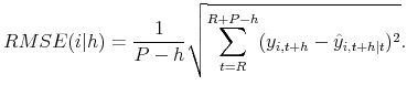
The forecast
PITs Based on Univariate Density Forecasts. Define the probability integral transformation for the actual ![]() -step ahead forecast of
-step ahead forecast of ![]() based on time
based on time ![]() information as
information as
If
Starting with Dawid (1984) and Kling and Bessler (1989) the use of PITs has a fairly long tradition in the literature on density forecast evaluation. PITs, sometimes known as generalized residuals, are relatively easy to compute and
facilitate comparisons among elements of a sequence of predictive distributions, each of which is distinct in that it conditions on the information available at the time of the prediction. It is shown in Rosenblatt (1952) and Diebold
et al. (1998) that for ![]() the
the
![]() 's are independent across time and uniformly distributed:
's are independent across time and uniformly distributed:
![]() . The uniformity result relies on the following argument. If a random variable
. The uniformity result relies on the following argument. If a random variable ![]() has an invertible cumulative density function
has an invertible cumulative density function ![]() , then
, then
| (5) |
The basic argument also works if
The uniformity property can be exploited in a predictive check. For instance, suppose one divides the unit interval into ![]() sub-intervals. According to the predictive distribution, the
expected fraction of PITs in each sub-interval is equal to
sub-intervals. According to the predictive distribution, the
expected fraction of PITs in each sub-interval is equal to ![]() . Paraphrasing Bayarri and Berger's (2004) frequentist principle, the fraction of actual PITs in each sub-interval
should be close to the fraction expected under the predictive distribution. The closeness can be assessed with a
. Paraphrasing Bayarri and Berger's (2004) frequentist principle, the fraction of actual PITs in each sub-interval
should be close to the fraction expected under the predictive distribution. The closeness can be assessed with a ![]() goodness-of-fit statistic of the form
goodness-of-fit statistic of the form
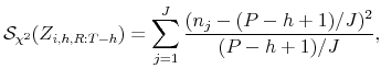
where
2.2 Evaluating Forecasts of Comovements
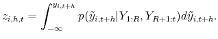
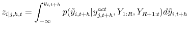
The main focus of our paper is the evaluation of DSGE models' forecasts of comovements. Multivariate density forecasts contain information about the correlation between aggregate output, inflation, interest rates, and other macroeconomic variables that appear in the DSGE model. In order to evaluate this information we consider statistics that capture the essence of the following thought experiment. Suppose a DSGE model generates a joint density forecast for output and interest rates. Moreover, suppose the forecaster knew the future interest rate. In this case the forecaster could replace the marginal predictive density of output by a conditional predictive density. Based on the conditional density one can construct a conditional mean forecast as well as a probability integral transform. If the DSGE model generates an accurate prediction of comovements, the actual reduction of the RMSE achieved by conditioning should be commensurable with the reduction predicted by the DSGE model. Moreover, the PITs should remain uniformly distributed. In addition, we compare the frequency of discrete events, such as output growth and inflation being above their steady state level, to their predicted probabilities.
Draws from the conditional predictive distribution of ![]() given
given
![]() are obtained by re-weighting draws from the bivariate distribution of predictive distribution of
are obtained by re-weighting draws from the bivariate distribution of predictive distribution of
![]() with a Gaussian kernel. Details are provided in the Online Appendix. As discussed above, our multi-step forecasts refer to
with a Gaussian kernel. Details are provided in the Online Appendix. As discussed above, our multi-step forecasts refer to ![]() -period averages
-period averages
![]() . Accordingly, we also consider averages of the conditioning variable, circumventing a curse-of-dimensionality problem when computing
conditional forecasts for large
. Accordingly, we also consider averages of the conditioning variable, circumventing a curse-of-dimensionality problem when computing
conditional forecasts for large ![]() with our Kernel method. For instance, the PIT for output conditional on interest rates at the four-period horizon, reflects the forecast of the average
growth rate conditional on a specific average interest rate over one year, rather than a forecast conditional on four distinct quarterly interest rate values. Since
with our Kernel method. For instance, the PIT for output conditional on interest rates at the four-period horizon, reflects the forecast of the average
growth rate conditional on a specific average interest rate over one year, rather than a forecast conditional on four distinct quarterly interest rate values. Since

RMSE Ratios. We use RMSEs and ratios of conditional and unconditional RMSEs as in Schorfheide et al. (2010) to form a predictive check. Let
![]() and
and
![]() denote the means of the conditional (given
denote the means of the conditional (given ![]() ) and
marginal predictive distribution of
) and
marginal predictive distribution of ![]() . The RMSE ratio is defined as
. The RMSE ratio is defined as
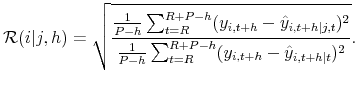
If the forecast errors are homoskedastic and normally distributed, then the RMSE ratio is one whenever the forecast errors are uncorrelated and less than one whenever the forecast errors are correlated. Suppose that the predictive distribution exhibits no correlation between
PITs Based on Conditional Density Forecasts. PITs based on conditional predictive distributions of ![]() given
given
![]() are defined as
are defined as
and have first been used by Diebold et al. (1999) to extend PIT-based density forecast evaluations to multivariate models. As in the case of unconditional univariate density forecasts, the marginal distribution of PITs based on conditional density forecasts is uniform and a predictive check can be based on the discrepancy between the empirical distribution of PITs and a uniform distribution.
Event Forecasts. Finally, we consider probability forecasts for events of the form
![]() . Let
. Let
![]() denote the model predicted probability that the event occurs. The event forecasts are evaluated based on
denote the model predicted probability that the event occurs. The event forecasts are evaluated based on
Here
Some remarks about
![]() are in order. Define the alternative statistic
are in order. Define the alternative statistic
![]() by squaring the difference between the indicator function and the predicted probability in (9) and by pre-multiplying it by minus
one:
by squaring the difference between the indicator function and the predicted probability in (9) and by pre-multiplying it by minus
one:
 |
(10) | |
 |
However, our goal is not to rank forecasting models. We are trying to assess whether predicted probabilities correspond with empirical frequencies. Dawid (1982) suggests to consider all forecasts for which the predicted probability of the event of interest is close to
![]() and to compute the fraction
and to compute the fraction ![]() of forecasts for which the event
occurred. If the function
of forecasts for which the event
occurred. If the function
![]() , the event forecasts are well calibrated. Since we have relatively few forecasts in our application, we are using a less stringent notion and simply examine the
discrepancy between the average frequency of an event and the average predicted probability. This discrepancy should be close to zero, if the event forecast is well calibrated.
, the event forecasts are well calibrated. Since we have relatively few forecasts in our application, we are using a less stringent notion and simply examine the
discrepancy between the average frequency of an event and the average predicted probability. This discrepancy should be close to zero, if the event forecast is well calibrated.
3 The DSGE Models
The predictive checks are applied to two New Keynesian DSGE models. First, we consider a small-scale model that consists of three basic equations: a consumption Euler equation, a New Keynesian Phillips curve, and a monetary policy rule. The theoretical properties of this class of models are discussed extensively in Woodford (2003), and numerous versions that differ with respect to the specification of the exogenous shock processes and the formulation of the monetary policy rule have been estimated based on output, inflation, and interest rate data, see Schorfheide (2008) for a survey. Second, we generate forecasts from the SW model. This model has a richer structure that accounts for capital accumulation, variable capital utilization, wage rigidity in addition to price rigidity, and households' habit formation.
3.1 A Small-Scale Model
Empirical specifications of the canonical small-scale New Keynesian DSGE model differ with respect to the exogenous shock processes as well as the formulation of the monetary policy rule. Our version is identical to the one studied in the survey paper by An and Schorfheide (2007) and includes a technology growth, a government spending, and a monetary policy shock. The interest rate feedback rule implies a reaction to output growth deviations from steady state rather than to deviations of the level of output from a measure of potential output.
Log-Linearized Equilibrium Conditions. We briefly summarize the log-linearized equilibrium conditions associated with the small-scale DSGE model. The underlying decision problems of households and firms are described in detail in An and Schorfheide (2007). Let
![]() denote the percentage deviation of a variable
denote the percentage deviation of a variable ![]() from
its steady state
from
its steady state ![]() . The equilibrium can be approximated by an intertemporal Euler equation, a New Keynesian Phillips curve, and an interest rate feedback rule:
. The equilibrium can be approximated by an intertemporal Euler equation, a New Keynesian Phillips curve, and an interest rate feedback rule:
![\displaystyle = E_t[\hat y_{t+1}] + \hat{g}_t - E_t[\hat{g}_{t+1}] - \frac{1}{\tau} \bigg( \hat R_t - \hat E_t[\pi_{t+1}] - E_t[\hat{z}_{t+1}] \bigg)](img120.gif)
Here
| (12) |
Measurement Equations. The model is completed by a set of measurement equations that relate the model states to a set of observables. We assume that the time period ![]() in the model
corresponds to one quarter and that the following observations are available for estimation: QoQ per capita GDP growth rates (YGR), QoQ inflation rates (INF), and quarterly nominal interest rates (FFR). The three series are measured in percentages, and their relationship to the model variables is
given by the following set of equations:
in the model
corresponds to one quarter and that the following observations are available for estimation: QoQ per capita GDP growth rates (YGR), QoQ inflation rates (INF), and quarterly nominal interest rates (FFR). The three series are measured in percentages, and their relationship to the model variables is
given by the following set of equations:
The parameter
Prior Distribution. Bayesian estimation of a DSGE model requires the specification of a prior distribution. The complete specification of the prior distribution is given in the Online Appendix. We use the same priors as in An and Schorfheide (2007) with one
exception: The inflation coefficient in the monetary policy rule is fixed at
![]() . It is well known in the literature that
. It is well known in the literature that ![]() is difficult to
identify. This lack of identification causes some numerical instabilities in the application of Markov-Chain Monte-Carlo (MCMC) methods. Since the predictive check requires us to estimate the DSGE model many times and the precise measurement of
is difficult to
identify. This lack of identification causes some numerical instabilities in the application of Markov-Chain Monte-Carlo (MCMC) methods. Since the predictive check requires us to estimate the DSGE model many times and the precise measurement of ![]() is not the objective of our analysis, we decided to fix the parameter.
is not the objective of our analysis, we decided to fix the parameter.
3.2 The Smets-Wouters Model
The SW model is the second model considered in this paper. The SW model is a more elaborate version of the DSGE model presented in Section 3.1. Capital is a factor of intermediate goods production, and nominal wages, in addition to nominal prices, are rigid. The model is based on work by Christiano et al. (2005), who added various forms of frictions to a basic New Keynesian DSGE model in order to capture the dynamic response to a monetary policy shock as measured by a structural vector autoregression (VAR). In turn, Smets and Wouters (2003) augmented the Christiano-Eichenbaum-Evans model by additional shocks to be able to capture the joint dynamics of Euro Area output, consumption, investment, hours, wages, inflation, and interest rates. The 2007 version of the SW model contains a number of minor modifications of the 2003 model in order to optimize its fit on U.S. data. We use the 2007 model exactly as presented in SW and refer the reader to that article for details. The log-linearized equilibrium conditions are reproduced in the Online Appendix.
Measurement Equations. The SW model is estimated based on seven macroeconomic time series. The period ![]() corresponds to one quarter and the measurement equations for output growth,
inflation, interest rates, consumption growth, investment growth, wage growth, and hours worked are given by:
corresponds to one quarter and the measurement equations for output growth,
inflation, interest rates, consumption growth, investment growth, wage growth, and hours worked are given by:
Since the neutral technology shock in the SW model is assumed to be stationary, the model variables are not transformed as in the small-scale model to induce stationarity, and the growth rate of the technology shock does not appear in the measurement equations.
Prior Distributions. Based on information that does not enter the likelihood function, SW fix the following five parameters in their estimation:
These parameter values are close to the posterior mean estimates reported in Smets and Wouters (2007). Our predictive check requires us to estimate the SW model several hundred times on recursive samples. Fixing the additional parameters ensures the numerical stability of our MCMC methods. The marginal prior distributions for the remaining parameters are identical to those used by SW and are summarized in the Online Appendix.
4 Empirical Results
The empirical analysis is presented in three steps. First, we discuss the data set that is used to conduct the predictive check (Section 4.1). Second, we evaluate the marginal predictive distributions of output growth, inflation, and interest rates (Section 4.2). Third, we examine the prediction of comovements of the small-scale DSGE model and the SW model (Section 4.3). Computational details pertaining to the implementation of Algorithm 1 are provided in the Online Appendix.
4.1 Data Set
For the evaluation of the density forecasts, we are using the real-time data set assembled by EG and extended by Del Negro and Schorfheide (2012). EG compared the accuracy of point forecasts from the SW model to those from the Fed's Greenbook. As part of their analysis the authors compiled for each Greenbook publication date real time observations for the time series that were used by Smets and Wouters (2007) to estimate their model. Since the focus in our paper is not a comparison of the DSGE model and the Greenbook forecast we use only a subset of the data sets constructed by EG, namely those for the Greenbooks published in March, June, September, and December. We refer to the March forecast as the first-quarter forecasts, and the remaining forecasts are associated with Quarters 2 to 4.
The March forecasts are based on fourth-quarter (Q4) releases from the previous year, meaning that the estimation period for the DSGE model effectively ends in Q4 of the preceding year. Thus, the first forecast (![]() ) in March is essentially a nowcast for Q1, and the subsequent forecasts are for Q2, Q3, and so forth. For each forecast origin, we refer to the "nowcast" as a one-step-ahead forecast and choose a maximum forecast horizon of
) in March is essentially a nowcast for Q1, and the subsequent forecasts are for Q2, Q3, and so forth. For each forecast origin, we refer to the "nowcast" as a one-step-ahead forecast and choose a maximum forecast horizon of ![]() . The first forecast origin in our analysis is March 1997 and the last forecast origin for one-step-ahead forecasts is June 2008, which provides us with 46 sets of forecasts. For horizons
. The first forecast origin in our analysis is March 1997 and the last forecast origin for one-step-ahead forecasts is June 2008, which provides us with 46 sets of forecasts. For horizons ![]() , the number of forecasts is reduced by
, the number of forecasts is reduced by ![]() . We decided to exclude observations from the 2008-09 recession
because the forecast errors of time series models in general are unusually large during this period. Since there is strong empirical evidence that monetary policy as well as the volatility of macroeconomic shocks changed in the early 1980s, we estimate both DSGE models based on data sets that start
in 1984:Q3.5 The predictive distribution for the model checks - using the notation of Section 2 - is constructed
conditional on
. We decided to exclude observations from the 2008-09 recession
because the forecast errors of time series models in general are unusually large during this period. Since there is strong empirical evidence that monetary policy as well as the volatility of macroeconomic shocks changed in the early 1980s, we estimate both DSGE models based on data sets that start
in 1984:Q3.5 The predictive distribution for the model checks - using the notation of Section 2 - is constructed
conditional on ![]() . Period
. Period ![]() corresponds to 1996:Q4, which is the last period
in the estimation sample that is used to generate the March 1997 forecasts.
corresponds to 1996:Q4, which is the last period
in the estimation sample that is used to generate the March 1997 forecasts.
In a real-time data environment, observations of ![]() published in period
published in period ![]() are potentially different from the observations that had been published in period
are potentially different from the observations that had been published in period ![]() . For this reason, time series are often indexed by a superscript, say
. For this reason, time series are often indexed by a superscript, say
![]() , which indicates the vintage or data release date. Using this notation, a Bayesian forecaster at time
, which indicates the vintage or data release date. Using this notation, a Bayesian forecaster at time ![]() has potentially access to a triangular array of data
has potentially access to a triangular array of data
![]() ,
,
![]() , ...,
, ...,
![]() . We decided not to modify the measurement equation of the DSGE models to capture the data revision process. When computing the recursive forecasts based on the actual data, we
are ignoring the presence of earlier data vintages and hence the potential information content in data revisions. Thus, we consider the sequence of predictive distributions
. We decided not to modify the measurement equation of the DSGE models to capture the data revision process. When computing the recursive forecasts based on the actual data, we
are ignoring the presence of earlier data vintages and hence the potential information content in data revisions. Thus, we consider the sequence of predictive distributions
![]() ,
,
![]() , instead of
, instead of
![]() . Likewise, when simulating trajectories from the DSGE model to construct the synthetic samples
. Likewise, when simulating trajectories from the DSGE model to construct the synthetic samples
![]() ,
,
![]() , we make no attempt to simulate vintages
, we make no attempt to simulate vintages
![]() that mimic the revision properties of U.S. data. While we acknowledge that it would be interesting to examine how results would change if the DSGE model were setup to process
the information contained in data revision, we find that such an extension is beyond the scope of this paper.
that mimic the revision properties of U.S. data. While we acknowledge that it would be interesting to examine how results would change if the DSGE model were setup to process
the information contained in data revision, we find that such an extension is beyond the scope of this paper.
The real-time-forecasting literature is divided as to whether forecast errors should be computed based on the first release following the forecast date, say
![]() or based on the most recent data vintage, say
or based on the most recent data vintage, say
![]() . The former might do a better job capturing the forecaster's loss, whereas the latter is presumably closer to the underlying "true" value of the time series. We decided to
follow the second approach and evaluate the forecasts based on actual values from the
. The former might do a better job capturing the forecaster's loss, whereas the latter is presumably closer to the underlying "true" value of the time series. We decided to
follow the second approach and evaluate the forecasts based on actual values from the
![]() data vintage. All real series are converted into per capita terms. Finally, as mentioned previously, all
data vintage. All real series are converted into per capita terms. Finally, as mentioned previously, all ![]() -step forecasts refer to averages over the forecast horizon. Thus, using the notation of Section 2, we consider forecasts of
-step forecasts refer to averages over the forecast horizon. Thus, using the notation of Section 2, we consider forecasts of
![]() rather than
rather than ![]() .
.
4.2 Evaluation of Marginal Density Forecasts
Figure 1 displays the RMSEs of pseudo out-of-sample forecasts of average output growth, inflation, and interest rates up to eight quarters ahead computed from the small-scale DSGE model and the SW model. The dashed lines indicate 90% credible bands associated with the model-implied predictive distribution of the RMSEs. The RMSEs attained with the small-scale model and the SW model are of similar magnitude as those reported in the previous literature. The small-scale model does about the same in forecasting GDP: the RMSE is 0.58 compared to 0.57 for the SW model. The SW model, on the other hand, delivers slightly more precise inflation and interest rate forecasts with RMSEs of 0.22 and 0.11, respectively, versus 0.26 and 0.13 for the small-scale model. For the small DSGE model, the RMSEs fall within the 90% credible interval generated by the predictive distribution, with the exception of the interest rate at longer horizons. For the SW model, the actual output RMSEs fall below the 5th percentile of their predictive distribution at most horizons. Conversely, the Federal Funds rate RMSEs are well within the bands associated with their predictive distribution.
The bands of the posterior predictive distribution supplement the information provided by the actual RMSEs in an important dimension. The actual output RMSEs in the SW model are in general smaller than what one would expect from the estimated model. A potential explanation for this finding is that some of the exogenous shock processes in the SW model are highly persistent, in part because they have to capture deviations of output, consumption, and investment from the model-implied common trend. Highly persistent shocks in turn imply fairly large forecast error variances, which contribute to the RMSE. Thus, the inconsistency of the actual RMSEs with those from the predictive check is a reflection of a model deficiency.
Figure 2 displays the histograms of the unconditional PITs from both models at one-quarter and four-quarter horizons. To generate the histogram plots, we divide the unit interval into ![]() equally sized subintervals and depict the fraction of PITs (measured in percent) computed from the actual data that fall in each bin. Since, under the predictive distribution, the PITs are uniformly distributed on the unit interval, we also plot the 20% line.
Finally, the dashed lines indicate the 5th and 95th percentile of the predictive distribution for the fraction of PITs in each bin.6 The
equally sized subintervals and depict the fraction of PITs (measured in percent) computed from the actual data that fall in each bin. Since, under the predictive distribution, the PITs are uniformly distributed on the unit interval, we also plot the 20% line.
Finally, the dashed lines indicate the 5th and 95th percentile of the predictive distribution for the fraction of PITs in each bin.6 The
![]() statistics, which were defined in (6) and measure the squared distance of the bin heights from the 20% line, are summarized in
Table 1. We also report the p-values (in parentheses) from the predictive distribution. In general, the
statistics, which were defined in (6) and measure the squared distance of the bin heights from the 20% line, are summarized in
Table 1. We also report the p-values (in parentheses) from the predictive distribution. In general, the
![]() statistics conform with the graphical information provided in the figures.
statistics conform with the graphical information provided in the figures.
At the short horizon, the density forecasts from the small DSGE model appear well calibrated for output and inflation, with the bars of the PIT histograms approximately equally sized and within the interval obtained from the predictive distribution. The empirical distribution of the PITs
associated with the one-step-ahead Federal Funds rate forecast is skewed to the right. The Federal Funds rate was persistently low over the evaluation period, a feature that the simple model was unable to capture. Looking at four-quarter-ahead averages, output and inflation density forecasts are
still fairly well calibrated, which is confirmed by the
![]() statistics reported in Table 1. The deficiency of the Federal Funds rate density forecast becomes slightly less pronounced at the longer
horizon, but still too many actual realizations fall into the left tail of the predictive distribution. The
statistics reported in Table 1. The deficiency of the Federal Funds rate density forecast becomes slightly less pronounced at the longer
horizon, but still too many actual realizations fall into the left tail of the predictive distribution. The
![]() statistic lies closer to center of the predictive distribution, with a p-value of 0.27 versus 0.06 for the one-quarter horizon.
statistic lies closer to center of the predictive distribution, with a p-value of 0.27 versus 0.06 for the one-quarter horizon.
The PIT histograms for the SW model are similar for inflation and the Federal Funds rate, but different with respect to output. The one- and four-quarter ahead forecasts for output of the SW model are poorly calibrated in comparison to the small-scale DSGE model. As shown in Table 1, the realized values of the
![]() statistics associated with marginal forecasts for output exceed or equal the 90th percentile of the predictive distribution at these two horizons. The density forecast
of output is too diffuse, as the PITs too frequently fall in the 0.2 to 0.4 (
statistics associated with marginal forecasts for output exceed or equal the 90th percentile of the predictive distribution at these two horizons. The density forecast
of output is too diffuse, as the PITs too frequently fall in the 0.2 to 0.4 (![]() ) and 0.4 to 0.6 (
) and 0.4 to 0.6 (![]() ) intervals, respectively. This feature is consistent with the RMSE predictive check discussed above. The estimated shock processes generate a predictive distribution that is too diffuse. If the model is simulated forward, the counterfactual output growth RMSEs are much larger
than the actual RMSEs because the simulated trajectories exhibit an unrealistically large output volatility.
) intervals, respectively. This feature is consistent with the RMSE predictive check discussed above. The estimated shock processes generate a predictive distribution that is too diffuse. If the model is simulated forward, the counterfactual output growth RMSEs are much larger
than the actual RMSEs because the simulated trajectories exhibit an unrealistically large output volatility.
Diebold et al. (1998) emphasized that for a correctly specified one-step-ahead density forecast the PITs are independent across time. Deviations from independence are indicative of a dynamic misspecification in the sequence of predictive distributions.
Figure 3 displays autocorrelation functions for PITs based on one-step-ahead density forecasts,
![]() in the notation of Section 2.1, of output, inflation, and interest rates as well as the corresponding 90% bands. For both DSGE models, the
PITs of output and inflation are only mildly correlated and lie within the 90% intervals. The correlation is somewhat more pronounced for the small-scale model, which is consistent with the SW model containing many more shocks and frictions that were designed to capture the dynamics of U.S. data.
For interest rates, on the other hand, a very different picture emerges. The PITs exhibit a strong first- and second-order serial correlation, complementing our previous finding that both models seem to systematically overpredict the Federal Funds rate.
in the notation of Section 2.1, of output, inflation, and interest rates as well as the corresponding 90% bands. For both DSGE models, the
PITs of output and inflation are only mildly correlated and lie within the 90% intervals. The correlation is somewhat more pronounced for the small-scale model, which is consistent with the SW model containing many more shocks and frictions that were designed to capture the dynamics of U.S. data.
For interest rates, on the other hand, a very different picture emerges. The PITs exhibit a strong first- and second-order serial correlation, complementing our previous finding that both models seem to systematically overpredict the Federal Funds rate.
To summarize, our predictive checks for the (marginal) density forecasts provide a more detailed picture of the DSGE models' forecast performance than a RMSE comparison. Consider, for instance, the four quarter-ahead forecast for output. The SW model attains an RMSE of 0.32 while the small-scale model generates a slightly larger RMSE of 0.36. At the same time, however, the density forecasts from the small model appear to be better calibrated than those from the SW model as the empirical distribution of the PITs is closer to a uniform distribution. The probabilities derived from the density forecasts of the small model are closer to the observed frequencies. The SW model predicts output volatility to be higher than it actually is. While the forecast performance of the two DSGE models is markedly different, no clear ranking emerges. Both models have deficiencies along different dimensions. The posterior predictive checks highlight deficiencies that are not apparent from RMSE comparisons.
4.3 Evaluating Predictions of Comovements
To assess the DSGE models' ability to predict comovements among macroeconomic aggregates, we now consider statistics computed from bivariate predictive distributions. Since a joint density of two random variables can be factorized into a marginal and a conditional density and since we have examined marginal densities in the previous subsection, we shall now focus on predictive densities that are conditioned on future realizations of output growth, inflation, or interest rates.
The starting point of the analysis is the relative precision of conditional and unconditional point forecasts. The unconditional point forecasts are the same that were used in Section 4.2 to compute the RMSEs displayed in Figure 1. To obtain forecasts conditional on future realizations, say of output growth, we compute the mean of the conditional predictive density. In a nutshell, if a joint predictive distribution is approximately normal and implies that two variables are highly correlated, then knowing the future realization of one of them should substantially reduce the RMSE when predicting the other.7 If the correlation structure in the predictive distribution is consistent with the observed comovements of the two variables, the predicted RMSE reduction should be commensurable with the actual reduction. An RMSE ratio of one is in some sense a lower bound for model behavior in the context of prediction. That is, any model can achieve an RMSE ratio of one by simply having the marginal and conditional predictive distributions coincide. In light of this, an RMSE ratio above one is particularly troubling.
Figure 4 displays the RMSE ratios of conditional and unconditional forecasts,
![]() in (7). For the small DSGE model, the RMSE ratios are at or above one for nearly all conditional forecasts. The only exception is the
Federal Funds rate forecast conditional on output and vice versa, which indicates small gains in precision through conditioning. For the forecasts of inflation given output and inflation given interest rates the poor performance of the conditional forecast is inconsistent with the RMSE ratios
implied by the predictive distribution. According to the predictive distribution of the small-scale model, the comovements between output and inflation should lead to potentially sizeable RMSE reductions through conditioning. The observed increase in the RMSE ratio associated with inflation
conditional on output suggests that the correlation structure implied by the small-scale DSGE model does not appropriately capture the comovements of output and inflation.
in (7). For the small DSGE model, the RMSE ratios are at or above one for nearly all conditional forecasts. The only exception is the
Federal Funds rate forecast conditional on output and vice versa, which indicates small gains in precision through conditioning. For the forecasts of inflation given output and inflation given interest rates the poor performance of the conditional forecast is inconsistent with the RMSE ratios
implied by the predictive distribution. According to the predictive distribution of the small-scale model, the comovements between output and inflation should lead to potentially sizeable RMSE reductions through conditioning. The observed increase in the RMSE ratio associated with inflation
conditional on output suggests that the correlation structure implied by the small-scale DSGE model does not appropriately capture the comovements of output and inflation.
The RMSE ratios for the SW model exhibit different behavior. There is hardly any gain using the conditional relationship between output and inflation and output and interest rates for forecasting. Moreover, this is, for the most part, consistent with the predictive distribution for the RMSE ratios. On the other hand, the predictive distribution indicates that there should be sizable gains from conditioning on interest rates to forecast inflation and vice versa. Unfortunately, the actual RMSE ratios for inflation conditional on interest rates (and vice versa) are greater than one at all horizons. The comovements of inflation and the interest rate implied by the SW model are at odds with the data.
It is worth discussing the causes of the differences in the predictive distributions reflected in the RMSE ratio bands. We tried to get insight into the issue by looking at estimation output and the predictive density from a "typical" subsample (using real data) in our estimation period. We picked the estimation sample ending in 2001:Q2, about halfway through the forecast evaluation period, although the results are broadly similar everywhere in the sample. For the small DSGE model, the predictive density indicates that there is a strong negative relationship between output and inflation. The correlation between four-step-ahead inflation and output embedded in the predictive density is -0.50. This is consistent with the expected reduction in RMSE indicated by the credible bands in Figure 4.
The negative relationship between output and inflation is driven by total factor productivity (technology), which acts as a supply shock in the model. An inspection of impulse response functions (not shown), indicates that an increase in technology reduces firms' costs, inducing them to produce more and lower prices. The other two shocks in the model generate a positive comovement between output and inflation. It is, however, the technology shock that dominates. An examination of the model-implied long-run relationship between output and inflation, calculated at the posterior mean, indicates that the correlation is -0.64 when all three shocks are included and just 0.07 when only the government spending and monetary policy shock are included.
There is no strong relationship between output and inflation in the density forecast of the SW model, despite the presence of a similar TFP shock in the model specification. The correlation between four-step-ahead output and inflation in the predictive density is only -0.04. Indeed, the impulse response functions for TFP look qualitatively similar to the ones generated by the small DSGE model, although the response of inflation is much more muted. Due to the rich structure and specification of the SW model, the technology shock contributes relatively little to the relationship between output and inflation. For instance, the presence of the investment-specific technology shock reduces the importance of the TFP shock. This shock generates a positive comovement between output and inflation, which cancels the effect of the TFP shock. Moreover, the preference and government spending shocks operate in the same fashion. It is true that the markup shocks - the other "new" shocks - generate negative comovement between output and inflation, but an inspection of the impulse responses suggests that the effect on output is dwarfed by the demand shocks listed above. On balance, the forces wash one another out, leaving comovements between output and inflation undetectable in the predictive density.
For inflation and interest rates, the findings are reversed. Here there is very little evidence of comovements in the small DSGE model while the SW model indicates that inflation should be very informative about the interest rate and vice versa. In the predictive densities, the correlation between four-step-ahead inflation and the interest rate is just -0.05 for the small DSGE model and 0.52 for the SW model. The comovement in the SW model is driven principally by the presence of price and wage markup shocks. Markup shocks directly cause wage and prince inflation to increase and the interest rate rises in reaction to this inflation, generating positive comovement. Moreover, both inflation and the interest rate are much more persistent in the SW model than in the small DSGE model. Interestingly, these same shocks generate a negative comovement between output and interest rates, an effect seen in the small DSGE model, that is counteracted by the demand shocks. In sum, the predictive densities of two models can be quite different, even if one model is "built upon" the other.
We proceed by examining the calibration of predictive distributions that are conditioned on the average realization of either output or interest rates. Figure 5 displays PITs based on density forecasts conditional on future output. For the small DSGE
model, the PIT histograms based on conditional density forecasts look similar to their unconditional counterparts in Figure 2. For the SW model, the PITs indicate that the density forecasts of the Federal Funds rate are better calibrated if they are conditioned on
output, in particular for ![]() . This is reflected in the difference between the
. This is reflected in the difference between the
![]() statistics for the conditional and unconditional forecasts reported in Table 1. For
statistics for the conditional and unconditional forecasts reported in Table 1. For ![]() the conditioning raises the p-value of
the conditioning raises the p-value of
![]() from 0.01 to 0.08. For
from 0.01 to 0.08. For ![]() the p-value increases from 0.10
to 0.40. Moreover, it is clear by examining the differences for the Federal Funds rate PITs in Figures 2 and 5 that the large number of interest rate observations falling into the center of the predictive density decreases when
conditioning on output.
the p-value increases from 0.10
to 0.40. Moreover, it is clear by examining the differences for the Federal Funds rate PITs in Figures 2 and 5 that the large number of interest rate observations falling into the center of the predictive density decreases when
conditioning on output.
The comovement of output growth and inflation with the Federal Funds rate is of particular importance to central banks, which often compare macroeconomic forecasts based on various hypothetical paths for short-term nominal interest rates. Thus, Figure 6 depicts PIT histograms for output and inflation obtained from forecasts that condition on average future interest rates. It is important to note that these histograms do not convey any information about the DSGE models' ability to generate accurate counterfactual policy predictions. We only examine whether the DSGE model is able to capture the comovement between interest rates and other macroeconomic variables under the actual policy.
For the small DSGE model, the histograms for PITs of one-step-ahean inflation and output forecasts conditional on interest rates look very similar to their unconditional counterparts. For ![]() conditioning leads to slightly too many output observations in the tails of the predictive distribution. The corresponding p-values drop from 0.64 to 0.33. For the SW model, at the short horizon the conditional distribution looks fairly similar to the unconditional distribution.
For output, this is unsurprising in light of the above discussion about the lack of comovements between output and interest rates in the SW model. Moreover, this is consistent with the observation that the RMSE ratios for one-quarter ahead forecasts are basically unity for output. For inflation,
the PITs look about the same as the unconditional PITs, although their overrepresentation in the right tail looks more pronounced. This is consistent with the RMSE ratio being slightly above one. At the longer horizon, the calibration of the conditional density forecast of output appears slightly
improved relative to the unconditional density forecast. The p-value increases from 0.10 to 0.32. On the other hand, the calibration of the forecast density for inflation has deteriorated subtantially relative the unconditional density. There are too many realizations in the right tail of the
predictive density. The deficiency gets even more pronounced at an eight-quarter-ahead forecasting horizon. Overall, this is in line with the poor RMSE of the inflation forecast conditional on interest rates. This indicates that the strong positive relationship between future interest rates and
inflation embedded in the predictive density in the SW model does not properly reflect the joint dynamics of the time series.
conditioning leads to slightly too many output observations in the tails of the predictive distribution. The corresponding p-values drop from 0.64 to 0.33. For the SW model, at the short horizon the conditional distribution looks fairly similar to the unconditional distribution.
For output, this is unsurprising in light of the above discussion about the lack of comovements between output and interest rates in the SW model. Moreover, this is consistent with the observation that the RMSE ratios for one-quarter ahead forecasts are basically unity for output. For inflation,
the PITs look about the same as the unconditional PITs, although their overrepresentation in the right tail looks more pronounced. This is consistent with the RMSE ratio being slightly above one. At the longer horizon, the calibration of the conditional density forecast of output appears slightly
improved relative to the unconditional density forecast. The p-value increases from 0.10 to 0.32. On the other hand, the calibration of the forecast density for inflation has deteriorated subtantially relative the unconditional density. There are too many realizations in the right tail of the
predictive density. The deficiency gets even more pronounced at an eight-quarter-ahead forecasting horizon. Overall, this is in line with the poor RMSE of the inflation forecast conditional on interest rates. This indicates that the strong positive relationship between future interest rates and
inflation embedded in the predictive density in the SW model does not properly reflect the joint dynamics of the time series.
We now consider a simple event study as a final dimension along which to evaluate the predictive densities. We partition the sample space for average output and inflation in four events: output growth and inflation are both above (below) their respective long-run targets, output growth is above
and inflation is below target, and output is below and inflation is above target. These events summarize the models' ability to correctly forecast the directional movements of output and inflation, which are important in policy settings. If both output and inflation are above (below) their
steady-state values, the policymaker has an incentive to raise (lower) interest rates. We assess how big the divergence is between the realized frequency of these events and the average probabilities of events implied by the model in Figure 7 for up to eight quarters
ahead, see
![]() in (9). The small scale model performs substantially worse for two of the events. The model overpredicts the event in which output and
inflation are both below target and underpredicts the event in which output is above and inflation is below target. Here is another example of a deficiency in comovements which would not be reflected in marginal distributions. These mispredictions roughly cancel out in the marginal for inflation.
On the other hand, the SW model appears well-calibrated for all events.
in (9). The small scale model performs substantially worse for two of the events. The model overpredicts the event in which output and
inflation are both below target and underpredicts the event in which output is above and inflation is below target. Here is another example of a deficiency in comovements which would not be reflected in marginal distributions. These mispredictions roughly cancel out in the marginal for inflation.
On the other hand, the SW model appears well-calibrated for all events.
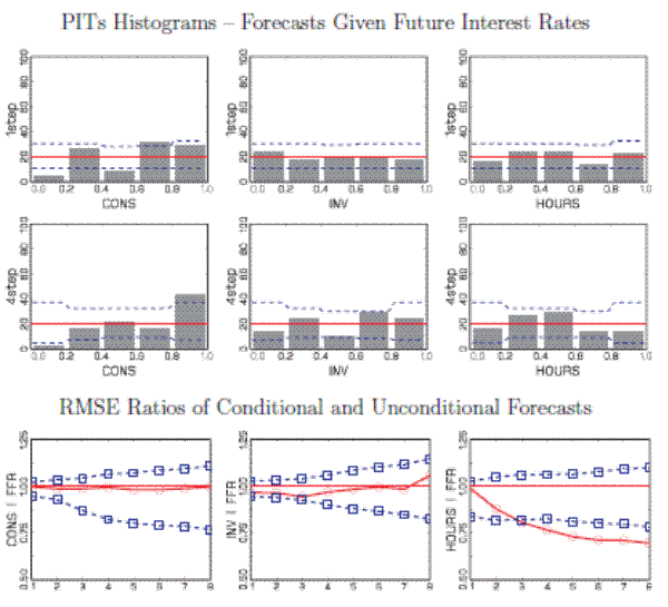
The SW model also generates a predictive distribution for consumption, investment, hours, and wages, in addition to the three variables we have considered. Now we augment our earlier results with a selection of results on the predictive distribution for consumption, investment, and hours. Figure 8 displays the PITs based on density forecasts of consumption, investment, and hours given future interest rates. We see that for one-quarter ahead forecasts for investment and hours, the predictive distributions appear to be well calibrated. For consumption, however, PITs are falling too frequently in one tail of the distribution. That is, relative the actual realizations of consumption, the model is underpredicting consumption. At the four-quarter range, these deficiencies become more pronounced. This problem is in part caused by the counterfactual common trend restriction that the SW imposes on consumption, investment, and output. In the data the growth rates of these series are slightly different.8 Conditioning on the Federal Funds rate leads to a substantial RMSE reduction of the hours worked forecast - which is inconsistent with the predictive distribution - but has essentially no positive effect on the consumption and investment forecasts.
5 Conclusion
This paper develops and applies tools to assess multivariate aspects of Bayesian DSGE model density forecasts and their ability to predict comovements among key macroeconomic variables. The forecast evaluation is implemented through posterior predictive checks that, broadly speaking, assess whether predicted probabilities are in line with observed frequencies in a recursive forecasting setting. For actual data and DSGE model-generated data we compare compare probability integral transformations based on marginal and conditional density forecasts as well as RMSEs associated with unconditional and conditional point forecasts. The predictive checks are applied to a simple three-equation New Keynesian model as well as the more elaborate SW model. It turns out that the predictive densities of the two DSGE models are quite different in various dimensions, yet no clear ranking emerges. The additional features incorporated into the SW model do not lead to a uniform improvement in the quality of the density forecasts and in the prediction of comovements. Moving forward, we hope that these predictive checks can be used as a diagnostic tool to assess DSGE model performance in a policy-relevant way and to spur new thinking about the specification of DSGE models, particularly with regard to modeling the relationship between key macroeconomic variables. The econometric tools developed in this paper can of course also be applied to other classes of multivariate time series models, such as vector autoregressions or dynamic factor models.
Bibliography
| Model | Output Gr. | Output Gr. (p-value) | Inflation | Inflation (p-value) | Interest | Interest (p-value) | |
| Uncond. (1 Quarter Ahead) | Small-Scale | 5.30 | ( 0.26 ) | 4.22 | ( 0.35 ) | 9.43 | ( 0.06 ) |
| Uncond. (1 Quarter Ahead) | Smets-Wouters |
12.22 | ( 0.01 ) | 3.78 | ( 0.40 ) | 13.11 | ( 0.01 ) |
| Cond on |
Small-Scale | 4.65 | ( 0.30 ) | 7.26 | ( 0.12 ) | ||
| Cond on |
Smets-Wouters | 5.56 | ( 0.21 ) | 8.44 | ( 0.08 ) | ||
| Cond on |
Small-Scale | 6.39 | ( 0.15 ) | 10.09 | ( 0.04 ) | ||
| Cond on |
Smets-Wouters | 8.89 | ( 0.06 ) | 6.22 | ( 0.17 ) | ||
| Cond on |
Small-Scale | 4.65 | ( 0.30 ) | 5.09 | ( 0.26 ) | ||
| Cond on |
Smets-Wouters | 11.56 | ( 0.01 ) | 8.44 | ( 0.08 ) | ||
| Uncond. (4 Quarter Ahead) | Small-Scale | 4.33 | ( 0.64 ) | 4.09 | ( 0.63 ) | 8.28 | ( 0.27 ) |
| Uncond. (4 Quarter Ahead) | Smets-Wouters | 14.90 | ( 0.10 ) | 3.48 | (0.71 ) | 14.90 | ( 0.10 ) |
| Cond on |
Small-Scale | 3.86 | ( 0.65 ) | 12.23 | ( 0.12 ) | ||
| Cond on |
Smets-Wouters | 4.19 | ( 0.65 ) | 6.81 | ( 0.40 ) | ||
| Cond on |
Small-Scale | 8.98 | ( 0.27 ) | 10.60 | ( 0.16 ) | ||
| Cond on |
Smets-Wouters | 9.43 | ( 0.28 ) | 18.95 | ( 0.04 ) | ||
| Cond on |
Small-Scale | 7.35 | ( 0.33 ) | 3.40 | ( 0.73 ) | ||
| Cond on |
Smets-Wouters | 8.71 | ( 0.32 ) | 26.10 | ( 0.01 ) |
 |
 |
|
Small-Scale DSGE Model
 |
 |
 |
 |
 |
 |