
How Does Social Security Claiming Respond to Incentives? Considering Husbands' and Wives' Benefits Separately
Keywords: Social Security incentives, retirement behavior, married couples
Abstract:
1 Introduction
Despite rising female labor force participation and relative earnings, a majority of women receive most of their Social Security benefits based upon their husbands' earnings history (Levine et al, 2000; Social Security Administration, various years). If husbands maximize lifetime household benefits (or Social Security Wealth, SSW) they should choose their benefit claiming age based on the total payments to be received by both spouses.1 If husbands fail to respond to dependent benefit incentives built into the system, they may choose a claim age that imposes significant financial losses on their spouse.2
Household Social Security benefits received in old-age are based on multiple eligibility criteria [retired worker, spouse, and survivor]. The husband and wife can each receive their own retired worker benefit and the dependent spouse (usually the wife) can receive spouse and survivor benefits if those benefits exceed her own retired worker benefits. Total lifetime benefits the household will receive are affected by the husband's claim age, because retired worker and dependent benefits both vary with the actuarial adjustments applied to monthly benefits. The incentives for claiming at any given age measure how household SSW is affected by those various actuarial adjustments.
Previous research has shown husbands' claiming behavior is in fact inconsistent with maximization of SSW (Munnell and Soto, 2005; Sass et al, 2007). Other research examining behavioral responses to Social Security incentives implicitly assumes husbands consider the incentives from his own benefit and any benefit received by his spouse equally when deciding when to claim benefits or retire (Coile and Gruber, 2007; Mastrobuoni, 2011). However, it is plausible he responds differently to each type of benefits.
Financial maximization suggests that if there is a large gain [penalty] to delaying claiming, an individual is more [less] likely to delay. I show that husbands' claiming behavior responds to the actuarial incentives built into their own retired worker benefit formula, estimating a large and significant negative response to retired worker incentives. However, I do not find a significant response to incentives from either total household benefits or the dependent benefits paid to wives. Husbands lose less than $100in lifetime retired workerbenefits when they claim at 62instead of the age which maximizes retired worker benefits [around age 63]. This is built into the system; the actuarial adjustment ensures little difference in lifetime benefits by claiming age. However, the failure to incorporate incentives from the dependent benefits reduces wives' lifetime benefits in excess of $5,000 for more than a third of wives.
Most of the variation in incentives can be explained by earnings history. This is particularly true once I separate incentives by type of benefit. Therefore, I must rely heavily on changes to the Social Security benefit formulas for exogenous variation in incentives in combination with the
typical approach which relies on a control function. These rules impact both the normal retirement age (NRA) and the delayed retirement credit (DRC). The new laws create eleven birth cohorts in the male population, each facing a different set of rules.![]() Changes to the NRA increase the penalty to early claiming, and increases in the DRC raise the financial gains to delaying claiming past the NRA. Variation in the birth year of each spouse creates distinct incentives for otherwise
identical couples born in different years. 3
Changes to the NRA increase the penalty to early claiming, and increases in the DRC raise the financial gains to delaying claiming past the NRA. Variation in the birth year of each spouse creates distinct incentives for otherwise
identical couples born in different years. 3
It is plausible that estimates from the base model capture segments of the population more likely to consider financial incentives in decision making or who understand the incentives better. 4 In addition, individuals who vary along health dimensions face different incentives. Those who we observe to live longer likely have private information about their health and may be more responsive to incentives.5 To address these concerns, I estimate the model on subsamples where measured incentives are closer to the true incentives or those perceived by the individual. In addition, I consider a role for joint leisure in the claiming decision since it has proved to be an important factor in determining couples' retirement decisions (Coile, 2004). These robustness checks provide similar results to main specification.
The structure for the remainder of the paper is as follows: Section II provides background on Social Security, Section III details the data, Section IV provides results comparing Social Security benefits lost by couples. Section V details the empirical approach, Section VI provides estimation results, and Section VII presents robustness checks. Section VII concludes.
2 How Does Husband's Claiming Age Affect His Wife's Benefits?
Since Social Security was founded in an era of one-earner families, a spouse benefit, equal to half of her husband's benefit, was added to the program since many wives did not have a benefit based on their own work history. If eligible6, she is also entitled to her own retired worker benefit, with the monthly benefit [Primary Insurance Amount (PIA)] a function of her lifetime earnings history subject to penalties for early claiming. To ease in
following discussion, I refer to the ratio
![]() as the "PIA ratio", reflecting the retired worker benefits of each spouse. Wives expect to receive a spouse benefit if the PIA ratio is below 0.5.7 The husband's claiming age does not impact the level of the spouse benefit directly. His claiming age only impacts her spouse benefits because she cannot claim spouse
benefits until after her husband claims his retired worker benefit.
as the "PIA ratio", reflecting the retired worker benefits of each spouse. Wives expect to receive a spouse benefit if the PIA ratio is below 0.5.7 The husband's claiming age does not impact the level of the spouse benefit directly. His claiming age only impacts her spouse benefits because she cannot claim spouse
benefits until after her husband claims his retired worker benefit.
In addition to a spouse benefit, a survivor benefit is paid equal to that received by the deceased when the primary earner dies. Survivor benefits can be claimed beginning at age 60. If the deceased claimed their own benefit early, penalties carry over to survivor benefit. In addition, if the deceased delayed claiming past the normal retirement age, credits applied to their monthly benefit carry over to the survivor benefit. Survivor benefit calculation is the most complicated, as both the husband's and wife's claiming age determines the monthly benefit. The formula for survivor benefits is:
2.1 Calculation of Household Social Security Wealth
The first step in calculating incentives is determining the expected lifetime Social Security benefits, SSW, associated with each potential claiming age. The expected monthly payment incorporates the PIA and actuarial adjustments, including all retired worker benefits, spouse and survivor benefits the wife expects to receive. All calculations assume the wife claims as soon as possible. Adding in her choice of claiming age complicates the process an immense amount and has little effect given most women should claim at age 62 to maximize household SSW. This conclusion comes from my calculations and the results of Sass et al (2007).8 She may switch to the spouse benefit when her husband claims if it is larger than her own retired worker benefit.9 The other event which permits a change of benefit type is the death of her spouse. Once household total monthly payments are calculated, all future values are discounted to age 62 using a 3% annual discount rate.10 The sex-specific mortality tables from the Social Security Administration (SSA) from 1980, 1990, and 2000 are used to estimate the probability of surviving to each future period. These survival probabilities are adjusted for differences in mortality by race and education using the adjustments from Brown et al (2002), following Liebman et al (2009).
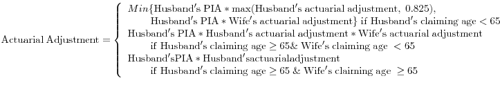
For an individual male worker with an average life expectancy, claiming age has little impact on his expected lifetime retired worker benefits. If he claims before his NRA, penalties are applied to the PIA in calculating the monthly benefit. Likewise, the monthly benefit is increased for any delay past his NRA. The DRC is the annual rate of increase applied to the PIA and varies by birth year. Between age 62 and 64, expected retired worker benefits change little [Figure 1]. For exposition, Figure 1 uses the 1990 life table with no race or education adjustments, a NRA of 65, and a DRC of 6.5%. These rules apply for those born in 1936 or 1937. After the NRA, lifetime benefits decline due to a less than actuarially fair DRC.
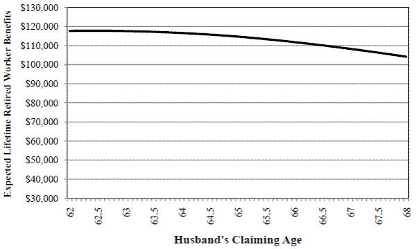
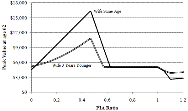
In contrast to lifetime retired worker benefits, household SSW can be impacted a great deal by his choice of claiming age. The impact of husband's claiming age on household SSW is shown in Figure 2 for two hypothetical couples where the wife is 3 years younger than her husband.11 In the first couple, the wife is not eligible for her own benefits, recreating the presentation from Coile et al (2002). For this couple, household benefits contain the husband's retired worker benefits, spouse and survivor benefits. In the first couple, the wife cannot receive spouse benefits until her husband claims his own benefits, so there is a small decline in expected spouse benefits after age 65 while she waits for him to claim. After age 62 and 2 months, survivor benefits increase monotonically as the husband's claim age increases. When claiming is delayed past age 65, the combination of declining spouse and worker benefits outweigh the increase in survivor benefits, seen in the lower series. The wife in the second couple has a PIA large enough to make the spouse benefit irrelevant [PIA ratio = 0.7]. For the second couple, SSW rises between ages 62 and 65 since survivor benefits increase faster than his worker benefits fall. However, the reverse is true after age 65 due to the less than actuarially fair DRC. Since husbands' claiming age does not have a large impact on expected spouse benefits in the first couple, household SSW is also maximized at age 65 for the second couple.12
2.2 Women and Social Security
Given the large increase in the labor force participation (LFP) of women and the narrowing of the gender wage gap, we might predict women will be more self-sufficient when they reach old age. With these changes, women are more independent of their husbands in determining their economic well-being while of working-age. Increased market wages and narrowing of the gender gap increase bargaining power in household financial decision-making (Pollak 2005, Knowles 2007). Due to Social Security rules, however, wives remain dependent on husbands in old-age (Levine et al, 2000). Even while women have increased their LFP and received higher wages, a husband typically works more years than his wife, between maternity leave and child rearing, and receives higher wages. As a result, most women end up relying on spouse and survivor benefits.
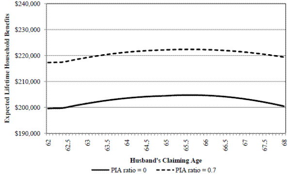
Over the past 50 years, the fraction of women eligible for their own benefit increased by almost 100%. In 1940, less than half of women recipients of Social Security were eligible for their own retired worker benefit, with eligibility defined by having at least 40 quarters of covered earnings. Almost three-quarters of current female beneficiaries are eligible to receive a benefit based on their own work history. However, the fraction of women receiving dependent benefits has been well over 50% for the past several decades.13 Only since the mid-1990s has this fraction begun to fall (Social Security Administration, various years). Furthermore, more than 90% of recent female recipients have a retired worker benefit smaller than their potential survivor benefit.14 In all of these cases, wives are impacted by their husbands' choices. Using data from SSA, I examine how this dependence has changed over time by examining the benefits paid to dual beneficiaries, those eligible for both their own worker benefit and a spouse or survivor benefit. Figure 3 compares the benefits received by current female dual beneficiaries to those she would have received from only her own retired worker benefits. As this ratio approaches 1, women will no longer be dependent on their husbands for the respective benefit. Figure 3 shows the ratio increasing from 1995 to the present for those that are receiving spouse benefits. However, there was an initial decline from 1986 to 1995, likely due to a change in the sample composition. As more women are eligible for retired worker benefits, the average lifetime earnings will fall as the newly eligibles have lower lifetime earnings. If the inflow to the sample from the bottom of the earnings distribution is larger than the outflow of women who are no longer dependent on spouse benefits, this decline is expected. This is likely true for the earlier period, as it coincides more with the beginning of the female labor force revolution. There is not an analogous fall and rise for survivor benefits. The likely explanation for this difference is beneficiaries receiving survivor benefits are older than those receiving spouse benefits. Therefore, we expect a rise in the future as women with stronger worker histories begin to receive survivor benefits.15
3 Data
The data utilized in this study is an administrative dataset which merges (1) a pared down version of the Survey of Income and Program Participation (SIPP) data from the 1990s (1990-1993, 1996), (2) the Summary Earnings Records (SER) and Detailed Earnings Records (DER) from the Internal Revenue Service, and (3) the Master Beneficiary Record (MBR) from SSA.16 This data is nearly ideal for the current study. Included in the data are birth date, OASDI claiming date and type of initial benefit, marital history, death date, earnings history, and a link to current spouse. Importantly, it is possible to determine whether individuals were married at the time of claiming using the marital history module from the SIPP. Marital status at claiming is crucial information in determining incentives faced by men. It is also necessary remove those who received disability benefits (DI) prior to age 62 since they do not face a claiming decision at age 62 and are automatically rolled into the old age program. The sample used for analysis includes all males born between 1922 and 1940. Those born prior to 1922 faced different Social Security rules, making calculations from the available data impossible. The last year we observe claiming is 2002. Those born in 1940 reach age 62 in 2002 allowing their inclusion since we observe their decision at age 62.
The sample contains 13,753 men who received retired worker benefits as their initial benefits from OASDI.17 Table 1 contains summary statistics for the analytical sample. The average lifetime retired worker benefits are $129,829.18 Almost 70% of households containing a married couple expect to receive survivor benefits, and about 45% expect to receive spouse benefits. Approximately three-quarters were married when they claimed retired worker benefits and about one quarter of men exit the labor force before age 62. On average, wives are 3.9 years younger than their husbands.19
Almost half of men claim benefits as soon as they are eligible (Figure 4).20 There is a second, well-known spike at age 65 with very few individuals
claiming after this age. One quarter of men claim between their 63![]() and 65
and 65![]() birthdays, while less than 5% claim after they turn 65. Those not married are more likely to claim before age 62½ than married men but married men are slightly more likely to claim around age 65. This is consistent with the predictions from financial maximization seen
in the previous section but weak evidence at best.
birthdays, while less than 5% claim after they turn 65. Those not married are more likely to claim before age 62½ than married men but married men are slightly more likely to claim around age 65. This is consistent with the predictions from financial maximization seen
in the previous section but weak evidence at best.
The key question underlying this analysis is whether the presence of wives' benefits causes different behavior among men. If singles claim in similar patterns to married men, the presence of dependent benefits likely plays no role in the claiming decision. Financial maximization predicts that married men should claim later than unmarried men, but Coile et al (2002) find this does not hold in the cross section. The empirical distributions in Figure 4 cannot confirm this result. This study answers whether differences in claiming by marital status is due to the presence of dependent benefits.
4 Benefits Lost due to Actual Claiming Age
For each couple in the sample, benefits `lost' compares potential benefits available to the household to the expected paid benefits that result from claiming choices. Potential benefits are the maximum household SSW, determined by the husband's claiming age. Most datasets do not include full earnings history for both spouses, and those that do, such as the matched HRS, are significantly smaller.21 In contrast, the current data contains over 10,000 matched couples and includes both spouses' earnings histories needed to calculate the PIA ratio. Assuming wives claim as soon as possible, more than 60% of husbands should claim at age 65 to maximize household SSW (Figure 5). These values are taken at annual intervals due to the Census Bureau's procedures to minimize disclosure risk. The concentration at age 65 is primarily due to the less than fair delayed retirement credit (DRC) for older cohorts. The gain to delay past age 65 is very small for older cohorts. The DRC has been increasing beginning with those born in 1925 but does not reach a more actuarially fair level until the 1939 cohort. For cohorts with the most favorable DRC, there is very small mass of those whose SSW maximizing claiming age is at the NRA. Other than cohort variation in the rules, the PIA ratio and age difference between spouses provide the remaining variation to determine the SSW maximizing claiming age.
Looking back at Figure 4, the empirical claiming distribution, there is little concentration near age 65 which would occur if men maximized household SSW. In addition, less than 10% of husbands `should' claim before age 63, far less than the observed 50% seen in Figure 4. Since behavior appears inconsistent with maximizing household SSW, I document the costs associated with actual claiming behavior. To do this, I look at how much money is `left on the table' as a result of early claiming.22 Sass et al (2007) explore this question for the HRS. The Synthetic SIPP also allows a larger number of birth cohorts to be analyzed. I first look at how much household wealth is "lost" due to early claiming by comparing the maximum available SSW and benefits received as a result of actual behavior.23 About 20% of couples lose a total of at least $5,000 and about 5% lose at least $20,000 (Figure 6). The numbers do not allow us to directly answer two questions. First is who bears the burden and second is what does this mean in terms of monthly benefits. To answer this first question, I group the benefits in the following way: (1) husband's retired worker benefits, (2) spouse benefits and wife's retired worker benefits received while husband is alive, and (3) survivor benefits and wife's retired worker benefits received after the husband dies.24 I refer to benefits paid to the wife while her husband is alive as "wife benefits" and benefits expected to be paid to the wife after her husband dies as "survivor benefits".
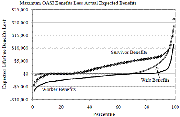
The distributions for lost wife and survivor benefits only include couples expected to receive each type of benefit given their age difference and PIA ratio. More than three quarters of husbands gain expected worker benefits due to choice of claiming age when compared to the benefits he would expect to receive if he maximized household SSW (Figure 7). These extra worker benefits are not large, with approximately 5% gaining more than $5,000 in expected lifetime worker benefits. One potential explanation for this finding is the majority of husbands respond only to their own benefit incentives. Since the SSW maximizing delay for most husbands is around age 65 to maximize household benefits and between ages 62 and 63 to maximize own benefits, husbands gain slightly from their choice of claiming age.25
Wives bear the majority of costs associated with early claiming since claiming age impacts affects husbands' retired worker benefits little. About one-third of wives lose more than $5,000 in expected lifetime survivor benefits, while more than 5% lose more than $10,000. It is difficult to conceptualize how big these numbers are in a practical sense because they incorporate survival probabilities. To address this, I compare the monthly survivor benefits received under actual husband behavior and hypothetical behavior. The three scenarios presented in Figure 8 are: (1) actual claiming behavior, (2) the age which maximizes SSW, and (3) age 68. Given actual claiming and assuming he passes away after his wife turns 65, approximately 25% of widows would find themselves living below the poverty line if she had no other income.26 In contrast, if husbands claimed at the age that maximized household benefits, less than 20% would be below the poverty line. If he claimed at age 68, later than the age that typically maximizes SSW, less than 15% would be in poverty. Not all widows rely solely on Social Security for their income but for many, Social Security plays a large role, particularly at the lower end of the income distribution. In 2008, almost half of unmarried female beneficiaries, including widows, received more than 90% of their income from Social Security (Social Security Administration, 2010).
5 Empirical Analysis
The empirical approach estimates a reduced form model of claiming. Panis (2002) use this model for claiming, and many others have estimated reduced form equations of retirement. Coile and Gruber (2007) estimate a probit model using Social Security benefits and financial incentives as their key independent variables, adapting the option value measure from Stock and Wise (1990) into financial terms.27 Given the link between claiming and retirement (Coile et al, 2002), it is natural to apply an analogous approach to Social Security claiming. The empirical models regresses an indicator for benefit claiming at age a on Social Security incentives at age a and control variables using a linear probability model: 28
![]()
The variables changing over time are the incentives from Social Security, age, and year. Once an individual has claimed benefits, they are removed from the sample. Since individuals are dropped after claiming, this model estimates hazard rates. The age controls are dummy variables for each age in the sample omitting age 62. This allows for the value of leisure to change over time while accounting for typical focal points associated with claiming at age 62 or 65. It should also help address sample selection issues that may arise if those in the sample for longer are different in unobservables from those who claim at age 62.
Two measures of financial incentives, peak value (PV) and accrual (ACC), are typically used in studies of claiming and retirement. They measure the financial gain from delaying claiming from period t to a future period. ACC compares SSW in t to SSW in t+1, where PV compares SSW![]() to the value at its maximum [SSW
to the value at its maximum [SSW![]() ]. Almost all studies calculate total household SSW defined as benefits paid from both the husbands' and wives' earning histories and use the resulting incentives as the key independent variable.29 By delaying today, one retains the option to claim benefits at a later date. One drawback to financial measures is that they do not account for the disutility of work, an important feature when considering
retirement incentives but less of an issue in this analysis focusing on benefit claiming.
]. Almost all studies calculate total household SSW defined as benefits paid from both the husbands' and wives' earning histories and use the resulting incentives as the key independent variable.29 By delaying today, one retains the option to claim benefits at a later date. One drawback to financial measures is that they do not account for the disutility of work, an important feature when considering
retirement incentives but less of an issue in this analysis focusing on benefit claiming.
It is straightforward to compare ACC across individuals for all types of benefits. When comparing two individuals, ACC calculates the annual change in SSW for each. Since the PV measure does not capture the timing of when the maximum value occurs for two individuals, using the PV measure complicates the analysis of benefit-specific incentives. For a given individual, there could be three different ages correspond to maximizing each type of benefit [worker, wife, and survivor]. The age that maximizes worker benefits is between age 62 and 63, and the survivor benefit is maximizes around age 70. The age which maximizes wife benefits varies with the age difference between spouses and the PIA ratio. SSW is the sum of husband's worker benefits, wife's benefits, and survivor benefits, but this linearity will not hold for the PV measure, i.e. PV of household will not equal the sum of the individual benefit PVs. However, the linearity will hold for the accrual measure.
ACC![]() = ACC
= ACC
![]() + ACC
+ ACC![]() + ACC
+ ACC![]()
Focusing on household incentives implicitly assumes husbands take all household benefits into consideration when making their claiming [or retirement] decision. This approach assumes husbands are indifferent between types of benefits received by the household over all points in time, regardless of whether he is alive when the benefits are received. This assumption needs to be evaluated. Much variation in household benefits is in terms of the survivor benefit, which the husband may not weight as heavily as benefits received while he is alive. After noting this, a natural extension is to consider each benefit separately. Incentive measures can easily be defined for each type of benefit after separating SSW into its components. The key contribution of this study is measuring incentives and the behavioral responses to these measures in a piece-wise approach. It is possible husbands are more sensitive to their own benefits, or at least more sensitive to benefits received while he is alive. Estimates for the response to household incentives are compared to results allowing for separate benefit incentives to see which model is more consistent with observed behavior. If behavior is consistent with treating all benefits equally, the coefficients on each type of benefit will be equal. This value would be equal to the coefficient on the household incentives in a separate model. This desired comparison provides additional incentive to focus on the accrual measure in addition to the linearity mentioned earlier.
Two channels impact the PIA when claiming is delayed. One is due to the change in PIA due to continued work, where a high earnings year can replace a low earnings year.30 The other is due to the actuarial adjustment of benefits. Liebman et al (2009) use the former source for identification since they focus on the labor supply incentives for retirement. Since claiming is the outcome of interest, it is important to use financial incentives only corresponding to claiming not labor force exit. Most papers combine the two channels but it is important use the appropriate incentives for each decision. Therefore, this study holds PIA fixed while changing the actuarial adjustment, focusing only on the incentives caused by a change in the claiming age not continued work. Separating the response to each channel, driven by different parameters of the Social Security program, will also be informative for reform.
While looking for suitable variation to identify the response to Social Security incentives, studies have focused on the significant heterogeneity in household incentives. Variation in incentives comes from the interaction of the couple's PIA ratio and age difference. Much of this heterogeneity is driven by eligibility for different types of benefits: worker, spouse or survivor. This interaction creates non-linearities in lifetime benefits around thresholds associated with "eligibility" for spouse and survivor benefits (Figure 10).31 This is the variation in incentives used for identification used by most studies of claiming and retirement. It is easy to see how the variation in total incentives can be attributed to the spouse and survivor incentives. This is additional motivation to use incentives associated with each separate benefit. Remaining cross sectional variation comes from earnings differences and changes in mortality between cohorts.
The empirical analysis uses a control function approach, following both Coile and Gruber (2007) and Liebman et al (2009) as guidelines. Coile and Gruber (2007) acknowledge the determinants of SSW are likely correlated with the retirement decision.32 Liebman et al (2009) are more explicit in describing the benefit formulas that drive model identification and how they use this information in defining their control function.
Omitted variables bias is less of a concern in a model of claiming than in a model of retirement unless claiming is a one-to-one mapping of retirement. In a model of retirement, the factors that determine incentives [measures of earnings history] play a direct role in the retirement decision. Furthermore, the concern for unobserved heterogeneity should be less of a concern when looking at the claiming decision since there is less uncertainty in incentives since all individuals in the sample are a minimum of 62 years old.33 Following previous research, I use a control function approach where including all variables used to calculate incentives so estimates are driven by variation uncorrelated with individual heterogeneity. The control function includes the same interactions of average lifetime earnings and potential earnings included in Coile and Gruber (2007). In addition, following Liebman et al (2009), measures of lagged earnings back to age 30 of the worker and his spouse and quartics of ln(SSW) are included. Since the empirical analysis considers each type of benefit separately, quartics of ln(Worker benefits), ln(Wife benefits) and ln(Survivor benefits) are controlled for.34 This control function captures approximately 90% of the variation in accrual for worker benefits, but captures less than one quarter of variation in the wife and survivor incentives.
The other source of identification is due to parametric changes in the Social Security benefit formulas. This source of identification has been use previously by Song and Manchester (2007), Kopczuk and Song (2008), and Mastrobuoni (2009), among others. There are two different types of changes. The first is an increase in the normal retirement age. It gradually increases from age 65 to 67 beginning with the cohort born in 1938. The second change is an increase in the delayed retirement credit from 3% per year to 8% per year beginning with those born in 1925. Both of these changes increase the return to delaying retirement, at different points in the claiming distribution. Most studies that rely on this variation for identification are strictly reduced form since the data analyzed do not allow the full calculation of household incentives due to incomplete spouse information. This study does not face this shortcoming.
To illustrate the impact of rule changes, consider a husband born in 1937 who claims his benefits at the EEA. He receives 80% of his PIA as a monthly benefit.35 An individual born in 1938 receives 79.17% if he claims at age 62 and 0 months and someone born in 1939 receives 78.33%. It is akin to multiple natural experiments. As the NRA increases, the incentives to claim at age 62 fall, where Figure A1 considers the increase from 65 to 66. If benefits are claimed at age 62 when an individual's NRA is 66, 75% of the PIA is paid on a monthly basis. For these two men, the ACC at age 62 is -$74 and -$1,765 respectively.
Changes to the DRC imply the incentives at the NRA are larger for younger individuals. An individual born in 1924 would receive 103% of his PIA as a monthly payment of his retired worker benefit if claimed at age 66 but someone born in 1935 would receive 106% of his PIA if benefits are claimed at age 66. Changes in the DRC also impact incentives for survivor benefits beginning at the NRA in a similar manner but the calculation is more involved.36
Identification of the spouse and survivor accrual comes from changes to the wife's NRA since the rules discussed above apply to women as well. The actuarial adjustment for each benefit is a function of the wife's birth year. The wide range of birth years of women married to men born between 1922 and 1940 create variation in the exact level of benefits.37 In addition, age difference between spouses varies the importance of spouse and survivor benefits for each couple. Those with younger wives have a larger weight on survivor benefits while those with older wives have a relatively larger weight on the spouse benefit, holding the PIA ratio constant.
Although claiming choice is a financial decision, in practice, factors other than Social Security incentives impact claiming. Credit constraints and preferences for leisure are two factors that likely influence claiming age independently of Social Security incentives. Mortality expectations impact claiming through the impact on expected future benefits (Hurd et al, 2004; Delavande et al, 2006). Control variables included to proxy for these additional inputs in decision making are education, marital status, work-limiting disability, experience and its square, household wealth including square and cubic, and observed mortality.
This study is forced to make assumptions about retirement behavior to isolate the Social Security claiming decision. One approach previously use is to focus only on those who have left the labor force before age 62 (Sass et al, 2007). However, this removes a large fraction of the Social Security beneficiaries. To proceed, I assume claiming is independent of the retirement decision. If claiming is a response to or part of exiting the labor force, there should be a weak response of claiming to Social Security incentives. Since incentives used only account for the actuarial adjustment and not the incentives associated with labor supply, bias due to this source is less of a concern. Holding PIA fixed at age 62 to isolate the role of actuarial adjustments understates the gain associated with claiming delay. To address concerns of retirement and claiming coordination, results including only those that exit the labor force by age 62 are provided. While there could be coordinating of retirement and claiming for early retirees, I expect the bias to be muted compared to the full sample.
6 Estimation Results
Results using both PV and ACC are reported for the base model but the remaining analysis is estimated with the ACC measure only. Table 2 begins with results for the response to household incentives in columns (1) and (4), the full and early retiree38 samples, respectively, to highlight what the approach used in the literature lacks and allow comparison to previous work. There is not a strong claiming response to the household incentives. The coefficient on the ACC measure in (1) suggests a $1000 increase in the annual change in household SSW leads to a 0.2 percentage point reduction in the claiming hazard. There is no response to household benefit incentives for early retirees, shown in Column (4), confirming the findings of Mastrobuoni (2011). Since early retirees only face incentives due to the actuarial adjustment and no changes to PIA, the incentives used here are identical to those used in Mastrobuoni's (2007) early retiree model. This is expected as both samples are both drawn from the SIPP, with only slight differences in sample selection.
For some individuals, primarily singles, household incentives include only worker benefit incentives. For others, the incentives are a combination of worker, spouse, and survivor benefits. Recognizing this fact makes it harder to interpret the response to household incentives. The remaining models separate out incentives by type of benefit. There is a strong negative response to the incentives from the retired worker benefit (Table 2). In model (2), a $1,000 increase in worker incentives reduces the hazard rate by 3.4 percentage points in the ACC model and 4.5 percentage points in the PV model. These results suggest a slightly stronger response to the total benefits to be gained instead of the annual gain. Since there is little difference between ACC and PV for retired worker benefits, we should not read too much into this result. There is no response to the incentives from either wife or survivor benefits. Models (3) and (6) combine the household and worker incentives in one model to see which measure is more important in determining male claiming. These results are consistent with the preceding models. Claiming behavior responds strongly to the worker incentives but not to any other incentives including those defined by household benefits. This is the primary message to be taken from this study. It is important to allow for the response to vary by type of benefits, for controlling for the overall incentives hides a true behavioral response.39
In the early retiree sample, there is smaller response to worker incentives than in the full sample. There is still little or no response to incentives determined by household, spouse or survivor benefits. There are arguments to be made why early retirees may be more or less responsive to incentives. It would not be surprising if they were more responsive as this group has been able to fund retirement prior to Social Security benefits. They may be more able to respond to incentives since they are not credit constrained; they were able to fund retirement prior to age 62. When these individuals reach age 62, they face strictly a financial decision of when to claim benefits. However, they could follow a rule of thumb to claim as soon as benefits are available since they are not making a joint claiming and retirement decision. Given early retirees are not credit constrained, Social Security benefits are likely a smaller portion of their annual income and overall wealth. If this is the case, maximizing SSW may not be a high priority. The results cannot distinguish whether the estimates from early retirees are a cleaner response to incentives and the presence of the retirement decision caused bias in the original models or if this subsample has a smaller causal response to retired worker incentives overall.
7 Robustness Checks
Before concluding husbands do not consider their spouses' benefit incentives when making their claiming choice, there are a few robustness checks to explore. The first goal is to identify groups in the population where there is more variation in claiming behavior, where all observed claiming is not at or near age 62. This ensures the model is not solely capturing individuals claiming at 62 due to a default rule who also happen to face incentives which encourage them to claim early. This also may identify populations more likely to respond to the other benefit incentives. The second goal is to identify populations who either understand the incentives better or may be more likely to respond to the incentives they face. This focuses on groups where the perceived incentives are closer to the calculated incentives, reducing bias from measurement error.
The first robustness check incorporates the impact of health on Social Security incentives as expected lifetime plays a central role in the calculation of SSW. Those who do not live as long receive benefits over fewer years. Claiming benefits early maximizes the lifetime benefits of those with
worse mortality prospects. Hurd et al (2004) and Delavande et al (2006) find those with low mortality expectations claim benefits slightly earlier than those who think they have a good chance of living to age 75. Unfortunately, there are no measures of mortality expectations in the SIPP so I cannot
allow the response to incentives to vary by mortality expectations. Ex post mortality is used as a proxy instead, since it is likely to be correlated with private information that informs mortality expectations. Those with short life expectancies [low mortality expectations] should claim as soon as
possible to maximize SSW and likely not respond to the calculated financial incentives. The first approach interacts the response to incentives with a dummy variable for whether the individual lives past his 75![]() birthday.40 This approach estimates whether the individuals in the two groups respond differently to the average incentives for
his race-education cell. Since measured incentives are more accurate for those who live to age 75, the second approach estimates the model only for individuals with better mortality outcomes. These results should be less prone to measurement error.
birthday.40 This approach estimates whether the individuals in the two groups respond differently to the average incentives for
his race-education cell. Since measured incentives are more accurate for those who live to age 75, the second approach estimates the model only for individuals with better mortality outcomes. These results should be less prone to measurement error.
In column (1) of Table 3, a $1,000 increase in household SSW over the next year reduces the claiming hazard by 0.2 percentage points with no statistically significant difference for those who live longer. There is no difference by observed mortality in the response to worker benefit incentives (column (2)). In column (3), there is a small but significant effect of household incentives on claiming in addition to the strong effect of worker incentives for those who live past 75. Those with average mortality do not experience a large variation in worker benefits by claiming age (Figure 1). It is possible the long-lived group can afford to be more responsive to dependent benefits with little cost in terms of their own benefit. The sign on the interaction between living past 75 with the survivor and spouse incentives is negative as predicted but insignificant and small in magnitude when compared to the coefficient on the worker incentives. The longer lived have a slightly stronger response to worker incentives slightly, shown in column (4), which is consistent with the hypothesis that the longer lived respond more to incentives. There are no other qualitative differences in the results from the two different approaches. Given the results from the long-lived sample, it does not appear measurement error significantly attenuates the coefficient estimates on worker incentives towards zero.41
A primary concern when estimating behavioral responses is whether individuals understand the program being analyzed. The implicit assumption when estimating the response to incentives is individuals understand the rules. Chan and Stevens (2008) note it is puzzling how strong the estimated behavioral response to pensions is given most individuals do not have a full understanding of the incentives. They find the response to private pensions is solely driven by those who understand their own pension. Given the complicated rules of the Social Security program it is reasonable to ask how well individuals understand the program. Leibman and Luttmer (2009) do just this. They find the median voter knows more than we think but the spouse benefit provision is not well understood. This finding could contribute to the lack of economic meaningful results concerning dependent benefits from the base model. Allowing for individual information is impossible given the data but instead look at whether those we expect to have more information respond to incentives differently. The best option given the data constraints focuses on differences by education.42 Those with more education likely have lower costs to gathering the relevant information or they have a higher chance of understanding the incentives themselves.
Men with a college degree are slightly less responsive to worker and wife's incentives but no more responsive to survivor incentives than those without a college degree. It suggests even those with less education respond to incentives and understand the incentives to some degree. The concern that only part of the population understands the benefit rules and responds to incentives does not appear to be true using educational attainment as a proxy for information. I find those with more education claim much later as expected given results from previous studies (Mastrobuoni, 2011; Sass et al, 2007). I also estimate the model only for those with a college education. This group might have an effective discount rate in line with our calculations, again providing estimates less susceptible to measurement error. The results in column (4) show a smaller response to retired worker incentives than the base model and look similar to results from the early retiree sample. Given the early retirees are more likely to have higher education, this finding is not surprising.
The final model alteration allows for a direct role of joint leisure in the response to incentives, looking indirectly at the interaction of the retirement and claiming decisions. Over the past twenty years, joint retirement has been observed. Valuing joint leisure could be a potential explanation why men claim benefits early. If their wife is not working, they might want to claim benefits and retired as soon as possible. Directly evaluating the role of joint leisure with the current data is difficult, but men may be less responsive to financial incentives if their objective function highly weights joint leisure. I break couples into three groups based on wives' work history. The first group is couples where the wife has a weak work history, defined as not being eligible for her own retired worker benefits. For wives eligible for her own benefit, the second group contains those with wives still working and the third where she has left the labor force.43 Although this is less than ideal approach to evaluate the role of joint leisure, it will to shed light on whether joint leisure impacts the claiming decision. Approximately 15% of wives have a strong work history but have exited the labor force while 30% of those with strong work histories are still working. Studies of joint retirement are limited because they only consider couples where both spouses have a strong work history or were both in the labor force at a given age, typically age 50 or 55. Examining claiming behavior does not face this constraint. The models are estimated for married men only; the omitted category is husbands whose wives have a weak work history. Table 5 presents results allowing for claiming and the response to incentives to vary by the three groups defined above. Starting with the group indicator variables [which are included in all previous models as well], husbands whose wives have a stronger work history appear more likely to claim that those whose wives have a weak work history but the differences in each model are not statistically significant. Men whose wives have left the labor market [and have a strong work history] are much less responsive to their own benefits. This is consistent with a joint leisure hypothesis if he ignores his own benefits once his wife retires. There is still no response to spouse or survivor incentives. These results point to a strong role for joint leisure in the decision of when to claim Social Security benefits and determining more precisely the role of joint leisure is an important avenue for future research.
8 Conclusions
This study highlights the dependence of wives on their husbands for Social Security benefits, a situation that persists even after the dramatic increase in labor force participation and wages women have experienced over the past several decades. My findings suggest that husbands are very responsive to their own benefit incentives, but they are not responsive to the incentives created by dependent benefits. This failure to respond to spousal and survivor incentives can significantly reduce wives' lifetime Social Security benefits.
I estimate models trying to elicit whether responses are driven by certain segments of the population who either respond more to financial incentives or for whom the incentives are calculated more accurately. I find those who live longer are slightly more responsive to the incentives from retired worker benefits but are not responsive to other benefit types. Those with the most education are much more likely to claim benefits later but those with all levels of education respond to the incentives. In addition, joint leisure appears to play a role in determining claiming age for those who experience a change to their potential leisure outcomes through the retirement of his wife. These men hardly respond to their own worker incentives.
Widows' well-being is partially determined by the claiming decision of her deceased spouse. In the case of survivor benefits, claiming age of the husband can increase the benefits by up to 50%. There is no evidence of behavior being consistent with husbands prioritizing the survivor benefit. There is a chance some of this discrepancy could be due to better understanding of own benefits, as noted by Liebman and Luttmer (2009), but it is unlikely that this is the sole explanation. Future cohorts may be more responsive to all benefits as they will receive the Social Security statement for longer, and maybe as a result will learn more about survivor benefits. As it currently stands, the Social Security statement does not provide much information about either spouse or survivor benefits, so this is one avenue for information dissemination. In addition, policy circles have talked about trying to disentangle the wives' benefits from their husbands' behavior due to the substantial impact of husband's claiming age on survivor benefits. Given the results of this study, this may be an avenue to more seriously consider.
9 References
Abowd, John, Martha Stinson and Gary Benedetto (2006). "Final Report to the Social Security Administration on the SIPP/SSA/IRS Public Use File Project."
Brown, Jeffrey, Jeffrey Liebman, and Joshua Pollet (2002). "Estimating Life Tables that Reflect Socioeconomic Differences in Mortality," in M.Feldstein and J. Liebman, The Distributional Effects of Social Security Reform University of Chicago Press: Chicago, IL.
Chan and Ann Huff Stevens (2008). "What You Don't Know Can't Help You: Pension Knowledge and Retirement Decision Making," The Review of Economics and Statistics 90(2)
Coile, Courtney (2004). "Retirement Incentives and Couples' Retirement Decisions," Topics in Economic Analysis & Policy 4(1)
Coile, Courtney and Jonathan Gruber (2007). "Future Social Security Entitlements and the Retirement Decision," The Review of Economics and Statistics 89(2)
Coile, Courtney, Peter Diamond, Jonathan Gruber, and Alain Jousten (2002). "Delays in Claiming Social Security Benefits," Journal of Public Economics 84(3)
Delavande, Adeline, Michael Perry and Robert Willis (2006). "Probabilistic Thinking and Early Social Security Claiming," University of Michigan, Michigan Retirement Research Center Working Paper 129.
Engelhardt, Gary and Jonathan Gruber (2004). "Social Security and the Evolution of Elderly Poverty," NBER Working Paper No. 10466.
Hurd, Michael, James Smith and Julie Zissimopoulos (2004). "The Effects of Subjective Survival On Retirement and Social Security Claiming." Journal of Applied Econometrics. 19 (6).
Knowles, John (2007). "Why are Married Men Working So Much? The Macroeconomics of Bargaining Between Spouses." IZA Discussion Paper 2909
Kopczuk, Wojciech and Jae Song (2008). "Stylized Facts and Incentive Effects Related to Claiming of Retirement Benefits Based on Social Security Administration Data." University of Michigan Retirement Research Center Working Paper 2008-200.
Levine, Philip, Olivia Mitchell, and John Phillips (2000). "A Benefit of One's Own: Older Women's Entitlement to Social Security Retirement." Social Security Bulletin 63 (3)
Liebman, Jeffrey and Erzo Luttmer (2009). "The Perception of Social Security Incentives for Labor Supply and Retirement: The Median Voter Knows More Than You'd Think," Unpublished Manuscript, Harvard University.
Liebman, Jeffrey, Erzo Luttmer, and David Seif (2009). "Labor Supply Responses to the Marginal Social Security Benefits: Evidence from Discontinuities." Journal of Public Economics 93(11-23).
Mastrobuoni, Giovanni (2011). "The Role of Information for Retirement Behavior: Evidence based on the Stepwise Introduction of the Social Security Statement." Journal of Public Economics 95(7-8), 913-925.
Mastrobuoni, Giovanni (2009). "Labor Supply Effect of the Recent Social Security Benefit Cuts: Empirical Estimates Using Cohort Discontinuities," Journal of Public Economics 93(11-12), 1224-1233l
Munnell, Alicia and Mauricio Soto (2005). "Why Do Women Claim Social Security Benefits So Early?" Center for Retirement Research Issue in Brief, Number 35.
Pollak, Robert (2005). "Bargaining Power in Marriage: Earnings, Wage Rates, and Household Production." NBER Working Paper No. 11239.
Sass, Steven, Wei Sun, and Anthony Webb (2007). "Why Do Married Men Claim Social Security Benefits So Early? Ignorance or Caddishness?" Center for Retirement Research Working Paper 2007-17.
Sass, Steven and Wei Sun. (2009). "How Much Do Household Lose By Claiming Social Security at Age 62?" Center for Retirement Research Working Paper 2009-11.
Social Security Administration (2010). "Social Security is Important to Women." Demographic Fact Sheet
Social Security Administration (various years). Annual Statistical Supplement to the Social Security Bulletin Washington, D.C. http://www.ssa.gov/policy/docs/statcomps/supplement/
Song, Jae and Joyce Manchester (2007). "New Evidence on Earnings and Benefit Claims Following Changes in the Retirement Earnings Test in 2000." Journal of Public Economics 91(3-4).
Stock, James and David Wise (1990). "Pensions, the Option Value of Work and Retirement." Econometrica 58(5), 1151-1180.
Warner, John. (1978). "Analysis of the Retention Impact of the Proposed Retirement System." Center for Naval Analysis, Memorandum 78-0362
Weaver, David (2001). "The Widow(er)'s Limit Provision of Social Security." Social Security Bulletin 64(1).
Figure 1. Expected Lifetime Retired Worker Benefits by Claiming Age, Men
Note: For males with PIA of $963 born in 1937; NRA = 65 and DRC = 6.5%.
Figure 2. Expected Household Social Security Wealth (SSW)
Notes: For males with PIA of $963 born in 1937; NRA = 65 and DRC = 6.5%; wife 3 years younger. PIA Ratio = Wife PIA/Husband PIA. If PIA ratio = 0, the household benefits are husband's retired worker, spouse and survivor benefits. If PIA ratio = 0.7, the household benefits are husband's retired worker, wife's retired worker, and survivor benefits.
Figure 3. Fraction of Total Benefits Due to own PIA, Female Dual Beneficiaries
Note: Each series represents the ratio [Own/Wife's PIA/Dependent Benefit] where "Dependent" refers to Spouse and Survivor Benefits respectively. Source: Social Security Administration, 2010
Figure 4. Empirical Distribution of Claiming Age by Marital Status at Claiming, Males
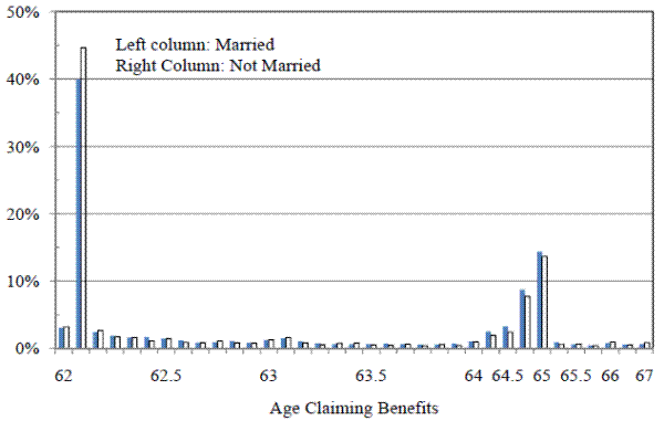
Figure 5. Distribution of Claiming Age that Maximizes Household SSW
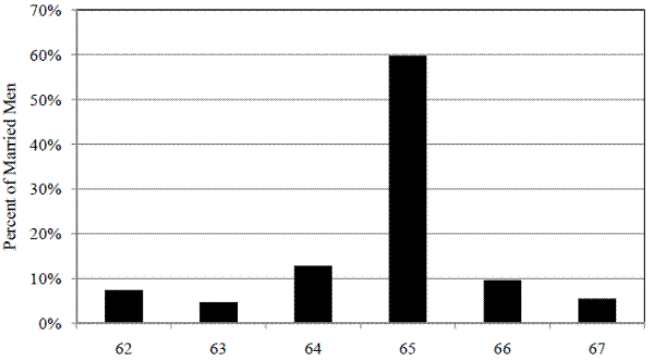
Figure 6. Distribution of Total Household Benefits Lost: Maximum OASI Benefits Less Actual Expected Benefits
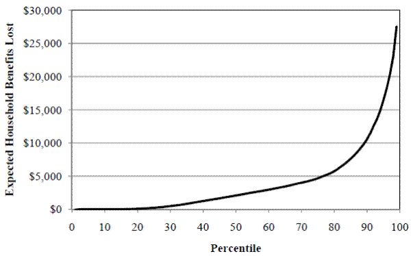
Figure 7. Lifetime OASI Benefits Lost, By Type: Maximum OASI Benefits Less Actual Expected Benefits
Note: Maximum Benefits are defined by the claiming age that maximizes the sum of wife & husband's worker benefits, spouse, and survivor benefits.
Figure 8. Actual and Potential Survivor Benefits
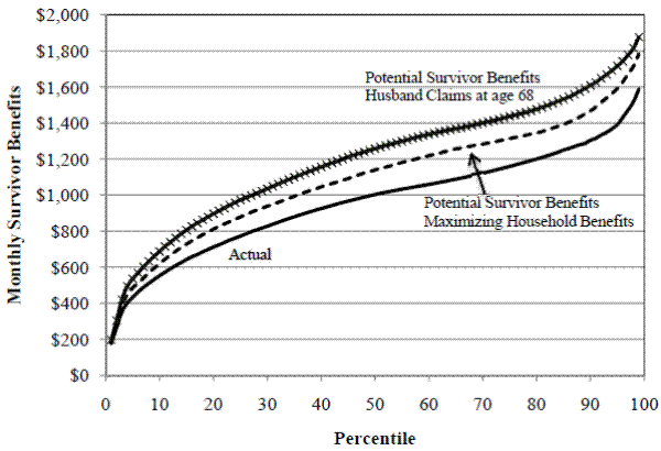
Figure 9. Household Peak Value, by PIA ratio and Age difference between Spouses
Note: PIA Ratio is the ratio of Wife's PIA to Husband's PIA
Table 1. Summary Statistics of Social Security Wealth, Incentives and Key explanatory variables
| Median | Mean | Std. Deviation | |
| Expected Worker Benefits | $133,755 | $129,829 | $43,858 |
| Fraction Expecting Spouse benefits | -- | 46.9% | 49.8% |
| Expected Spouse Benefits | $0 | $21,612 | $25,428 |
| Fraction Expecting Survivor benefits | -- | 0.6920 | 42.1% |
| Expected Survivor Benefits | $41,178 | $36,877 | $28,167 |
| Accrual - Worker Benefits | $206 | $563 | $467 |
| Accrual - Spouse Benefits | $0 | $76 | $1,334 |
| Accrual - Survivor Benefits | $1,737 | $1780 | $4,004 |
| Age Difference Between Spouses | 2.71 | 3.9 | 5.6 |
| Total Net Worth | $141,914 | $370,958 | $739,495 |
| Fraction Claiming Single | -- | 24.3% | 39.4% |
| Fraction with at least College Degree | -- | 28.9% | 42.9% |
| Fraction Retiring prior to age 62 | -- | 32.1% | 44.9% |
| Years with earnings before claiming | 37 | 28.0 | 9.0 |
| Years with earnings before claiming - Spouse | 15 | 15.2 | 13.8 |
| Health Limits Work | -- | 17.0% | 32.3% |
| Health Limits Work - Spouse | -- | 19.8% | 35.2% |
Number of Individuals: 13,753. Sample: Men born between 1922 and 1940. Incentives reported at age 62. Note: PV = SSW![]() - SSW
- SSW![]() . ACC = SSW
. ACC = SSW![]() - SSW
- SSW![]()
Table 2. Baseline Model Results
| Sample | (1) Full Sample | (2) Full Sample | (3) Full Sample | (4) Early Retirees | (5) Early Retirees | (6) Early Retirees |
| Accrual Household | -0.0022*** | 0.0004 | -0.0004 | -0.0003 | ||
| Accrual Household (Standard Error) | (0.0007) | (0.0010) | (0.0011) | (0.0011) | ||
| Accrual Worker | -0.0337*** | -0.0339*** | -0.0121*** | -0.0121*** | ||
| Accrual Worker (Standard Error) | (0.0022) | (0.0019) | (0.0048) | (0.0049) | ||
| Accrual Wife | 0.0003 | -0.0021 | ||||
| Accrual Wife (Standard Error) | (0.0013) | (0.0017) | ||||
| Accrual Survivor | 0.0012 | 0.0008 | ||||
| Accrual Survivor (Standard Error) | (0.0008) | (0.0013) | ||||
| Peak Value Household | 0.0004 | 0.0010 | 0.0003 | 0.0007 | ||
| Peak Value Household (Standard Error) | (0.0004) | (0.0004) | (0.0004) | (0.0005) | ||
| Peak Value Worker | -0.0451*** | -0.0629*** | -0.0284*** | -0.0230*** | ||
| Peak Value Worker (Standard Error) | (0.0040) | (0.0040) | (0.0089) | (0.0089) | ||
| Peak Value Wife | 0.0010** | -0.0003 | ||||
| Peak Value Wife (Standard Error) | (0.0006) | (0.0007) | ||||
| Peak Value Survivor | 0.0009 | 0.0026*** | ||||
| Peak Value Survivor (Standard Error) | (0.0006) | (0.0008) |
# Observations Full Sample: 27,310. # Observations Early Retirees: 19,675. # Individuals Full Sample: 13,753. # Individuals Early Retirees: 7,643. Source: Averaged values from 4 completed data implicates from Gold Standard data. Standard errors are calculated as detailed in Abowd et al (2006).
Note: Population mortality tables used in calculation of incentives. Control variables in each model are age dummies, education, interactions of quartics of AIME and potential earnings, own and spouse earnings starting at age 30, experience and its square, death after age 75 of self & spouse, death after age 80 of self & spouse, years since retirement (if retired), presence of work limiting disability, presence of DB/DC pension, net household wealth up to its cubic, and log(SSW), log(Worker Benefits), log(Spouse Benefits) and log(Survivor benefits) up to their cubics.
Table 3. Results by Husbands' Ex Post Mortality
| Sample | (1) Full | (2) Full | (3) Full | (4) Those who live to at least age 75 |
| Accrual-Household | -0.0020 | -0.00001 | ||
| Accrual-Household (Standard Error) | (0.0021) | (0.0007) | ||
| *Death after age 75 | -0.0036 | -0.0024* | ||
| *Death after age 75 (Standard Error) | (0.0023) | (0.0014) | ||
| Accrual - Worker | -0.0206*** | -0.0205 | -0.0244*** | |
| Accrual - Worker (Standard Error) | (0.0022) | (0.0022) | (0.0041) | |
| *Death after age 75 | -0.0011 | 0.0002 | ||
| *Death after age 75 (Standard Error) | (0.0018) | (0.0019) | ||
| Accrual - Wife | 0.0011 | 0.0014 | ||
| Accrual - Wife (Standard Error) | (0.0014) | (0.0040) | ||
| *Death after age 75 | -0.0027 | |||
| *Death after age 75 (Standard Error) | (0.0039) | |||
| Accrual - Survivor | -0.0005 | -0.0015 | ||
| Accrual - Survivor (Standard Error) | (0.0009) | (0.0013) | ||
| *Death after age 75 | -0.0014 | |||
| *Death after age 75 (Standard Error) | (0.0015) | |||
| Death after age 75 | 0.0100 | 0.0045 | 0.0057 | n/a |
| Death after age 75 (Standard Error) | (0.0097) | (0.0116) | (0.0115) | n/a |
| Spouse's death after age 75 | 0.0043 | -0.0010 | -0.0009 | 0.0025 |
| Spouse's death after age 75 (Standard Error) | (0.0100) | (0.0101) | (0.0322) | (0.0192) |
# Observations Full: 27,042. # Observations Those who live at least age 75: 9,466. # Individuals Full: 13,753. # Individuals Those who live at least age 75: 4,334. Source: Averaged values from 4 completed data implicates from Gold Standard data. Standard errors are calculated as detailed in Abowd et al (2006).
Note: Control variables in each model are age dummies, education, interactions of quartics of AIME and potential earnings, own and spouse earnings starting at age 30, experience and its square, years since retirement (if retired), presence of work limiting disability, presence of DB/DC pension, net household wealth up to its cubic, and log(SSW), log(Worker Benefits), log(Spouse Benefits) and log(Survivor benefits) up to their cubics.
Table 4. Results by College Education
| Sample | (1) Full | (2) Full | (3) Full | (4) College Graduates |
| Accrual - Household | -0.0025 | -0.0015 | ||
| Accrual - Household (Standard Error) | (0.0025) | (0.0034) | ||
| *College | 0.0024** | 0.0025* | ||
| *College (Standard Error) | (0.0012) | (0.0014) | ||
| Accrual - Worker | -0.0374*** | -0.0372*** | -0.0138*** | |
| Accrual - Worker (Standard Error) | (0.0067) | (0.0023) | (0.0040) | |
| *College | 0.0062*** | 0.0050*** | ||
| *College (Standard Error) | (0.0015) | (0.0016) | ||
| Accrual - Wife | -0.0017 | 0.0017 | ||
| Accrual - Wife (Standard Error) | (0.0015) | (0.0022) | ||
| *College | 0.0048** | |||
| *College (Standard Error) | (0.0024) | |||
| Accrual - Survivor | 0.0008 | 0.0004 | ||
| Accrual - Survivor (Standard Error) | (0.0010) | (0.0013) | ||
| *College | 0.0013 | |||
| *College (Standard Error) | (0.0017) | |||
| College | -0.3525*** | -0.3406*** | -0.3424*** | n/a |
| College (Standard Error) | (0.0208) | (0.0198) | (0.0198) | n/a |
# Observations Full: 27,042. # Observations College Graduates: 11,630. # Individuals Full: 13,753. # Individuals College Graduates: 3,858. Data: Averaged values from 4 completed data implicates from Gold Standard data. Standard errors are calculated as detailed in Abowd et al (2006).
Note: Control variables in each model are age dummies, education, interactions of quartics of AIME and potential earnings, own and spouse earnings starting at age 30, experience and its square, years since retirement (if retired), presence of work limiting disability, presence of DB/DC pension, net household wealth up to its cubic, and log(SSW), log(Worker Benefits), log(Spouse Benefits) and log(Survivor benefits) up to their cubics.
Table 5. Results by Wife's Labor Force History
| (1) | (2) | (3) | |
|---|---|---|---|
| Accrual - Household | -0.0030 | 0.0008 | |
| Accrual - Household (Standard Error) | (0.0028) | (0.0010) | |
| *Wife Strong LF, Exited LF | 0.0045** | -0.0022 | |
| *Wife Strong LF, Exited LF (Standard Error) | (0.0019) | (0.0044) | |
| *Wife Strong LF, Still Working | 0.0015 | 0.0014 | |
| *Wife Strong LF, Still Working (Standard Error) | (0.0013) | (0.0014) | |
| Accrual - Worker | -0.0279*** | -0.0283*** | |
| Accrual - Worker (Standard Error) | (0.0023) | (0.0025) | |
| *Wife Strong LF, Exited LF | 0.0193*** | 0.0197*** | |
| *Wife Strong LF, Exited LF (Standard Error) | (0.0044) | (0.0043) | |
| *Wife Strong LF, Still Working | -0.0004 | -0.0004 | |
| *Wife Strong LF, Still Working (Standard Error) | (0.0023) | (0.0016) | |
| Accrual - Wife Benefits | -0.0012 | ||
| Accrual - Wife Benefits (Standard Error) | (0.0020) | ||
| *Wife Strong LF, Exited LF | -0.0007 | ||
| *Wife Strong LF, Exited LF (Standard Error) | (0.0041) | ||
| *Wife Strong LF, Still Working | 0.0017 | ||
| *Wife Strong LF, Still Working (Standard Error) | (0.0028) | ||
| Accrual - Survivor | 0.0025 | ||
| Accrual - Survivor (Standard Error) | (0.0013) | ||
| *Wife Strong LF, Exited LF | -0.0014 | ||
| *Wife Strong LF, Exited LF (Standard Error) | (0.0023) | ||
| *Wife Strong LF, Still Working | 0.0007 | ||
| *Wife Strong LF, Still Working (Standard Error) | (0.0016) | ||
| Wife Strong LF, Exited LF | -0.0259 | -0.0163 | -0.0185 |
| Wife Strong LF, Exited LF (Standard Error) | (0.0191) | (0.0244) | (0.0234) |
| Wife Strong LF, Still Working | -0.0117 (0.0145) | -0.0162 (0.0171) | -0.0176 (0.0167) |
| Wife Strong LF, Still Working (Standard Error) | (0.0145) | (0.0171) | (0.0167) |
Data: Averaged values from 4 completed data implicates from Gold Standard data. Standard errors are calculated as detailed in Abowd et al (2006).
Note: "Wife Strong LF" is wives who have at least 10 years of positive earnings and are eligible for their own retired worker benefit from SS.
Control variables in each model are age dummies, education, interactions of quartics of AIME and potential earnings, own and spouse earnings starting at age 30, experience and its square, years since retirement (if retired), presence of disability, presence of DB/DC pension, net household wealth up to its cubic, and log(SSW), log(Worker Benefits), log(Spouse Benefits) and log(Survivor benefits) up to their cubics.
Figure A1. Expected Lifetime Retired Worker Benefits, by Normal Retirement Age (NRA)
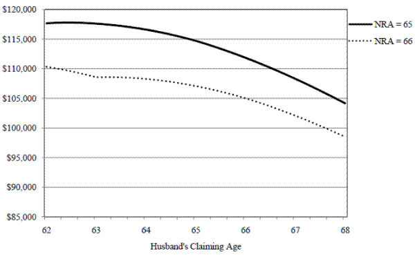
Figure A2. Expected Survivor Benefits by Delayed Retirement Credit (DRC)
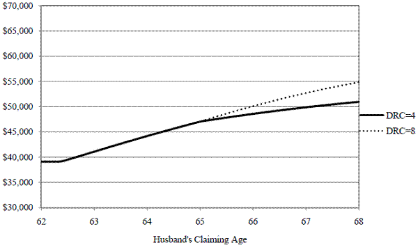
Note: For males with PIA of $963 born in 1937, NRA = 65, and wife 3 years younger.
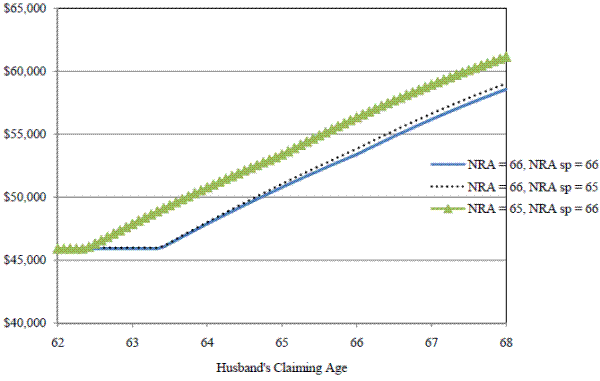
Figure A3. Survivor Benefits by NRA of Husband and Wife
Alice M. Henriques CV March 2012
Alice M. Henriques
Board of Governors of the Federal Reserve System
20![]() and C St. N.W. M.S. 153
and C St. N.W. M.S. 153
Washington, DC 20551
Home Address:
321 13![]() St SE
St SE
Washington, DC 20003
(215) 801-6474
(202) 452-3080
Education
Ph.D. Economics, Columbia University, 2012
M.A. Economics, Columbia University, 2007
B.A. University of California at Berkeley, High Honors, 2002
Professional Experience
Federal Reserve Board of Governors
Economist, 2011-present
Honors
Center for Retirement Research Dissertation Fellowship, 2009
National Science Foundation Graduate Research Fellowship, Honorable Mention, 2005
Research Fields
Public Economics, Labor Economics, Household Finance
Research
Publications
"Gender Gap in Wage Returns to Job Tenure and Experience," with Lalith Munasinghe
and Tania Reif. Labour Economics. December 2008.
Working Papers
"How Does Social Security Claiming Respond to Financial Incentives? Considering
Husbands' and Wives' Benefits Separately."
How does Job Loss Impact Employer-Provided Health Insurance Coverage & Wages?
Evidence from the Survey of Income and Program Participation
"Accounting for Changes in Poverty and Income Distribution of Elderly Women"
Referee Service
Journal of Public Economics
Other Experience
Social Security Administration
Graduate Research Intern, Summer 2008
Instructor for Undergraduate Econometrics
Columbia University, Summer 2010
The Brookings Institution
Research Assistant, 2002-2005
ReferencesProfessor Till von Wachter
Department of Economics
Columbia University
(212) 854-5712
Professor Wojciech Kopczuk
Department of Economics
Columbia University
(212) 854-2519
Professor Stephen Zeldes
Graduate School of Business
Columbia University
(212) 854-2492