
Can Macro Variables Used in Stress Testing Forecast the Performance of Banks?*
Keywords: Forecast combinations, macbro variables, measures of banking conditions, stress tests
Abstract:
1 Introduction
Stress tests are one of the tools used by banks to understand their risk exposures. Bank regulators use stress tests to verify that banks will still be able to maintain adequate levels of capital under stressful but plausible circumstances.
One type of stress test, referred to as "scenario analysis," involves the application of historical or hypothetical scenarios to assess the impact of various events on the performance of banks. Scenario analysis was an integral part of the Comprehensive Capital Analysis and Review (CCAR), a supervisory assessment of bank holding companies conducted by the U.S. Federal Reserve in 2011 and 2012, as well as of the Supervisory Capital Assessment Program (SCAP) in 2009. In these three instances, the 19 largest U.S. bank holding companies were asked to submit capital plans extending 9 quarters out and reflecting macroeconomic baseline and stress scenarios formulated by the Federal Reserve.1 As mandated by the Dodd-Frank Wall Street Reform and Consumer Protection Act, scenario analysis will continue to be an integral part of stress tests for the largest bank holding companies in the United States.2
An unstated premise of stress tests built around a macroeconomic scenario is that the macro variables should be useful factors in forecasting the performance of banks. We assess whether variables such as the ones included in the CCAR scenarios help improve out of sample forecasts of chargeoffs on loans, revenues, and capital measures, relative to forecasting models that exclude a role for macro factors. Furthermore, we construct confidence bands around the conditional forecasts of our measures of performance for the banking sector.3
The forecast method that we use is the equal-weighted average of simple models as first proposed by Bates and Granger (1969). This approach has been found to yield results near the frontier of best performance in a varied range of applications, see, for instance Stock and Watson (2004), who also provide extensive references to the literature on forecast combinations. Faust and Wright (2008) opine that "its empirical success is part of the folklore of forecasting," and like many others include the equal-weighted combination of simple models as a standard benchmark.
Specifically, we focus on Root Mean Squared Errors (RMSEs) for a battery of forecast combination models conditional on macro variables, chosen because they are included in CCAR scenarios, and a random walk model. Comparisons against a random walk model are interesting on at least three accounts: 1) the random walk model beats purely auto-regressive models in RMSE; 2) it has no role for macro variables; 3) it is a standard benchmark model for forecast assessment.
The scenarios used in the recent stress tests of bank holding companies in the United States were not tailored to the business model of any one specific company. We focus on forecasting aggregate performance for the companies involved in stress testing in the United States. It is not our purpose to tailor our regressions to encompass bank-specific factors. A priori, it is not clear whether or not bank specific factors would reveal more robust relations between bank performance measures and macro factors. We leave that pursuit for further work.
Interest in stress testing, prior to the financial crisis, was mostly circumscribed to practitioners. Early contributions that document the use of time series models for stress testing are those of Blaschke et al. (2001), Kalirai and Schleicher (2002), and of Bunn et al. (2005). In a recent paper, Covas et al. (2012) model PPNR's six sub components as well as net chargeoffs to generate a path of the tier-1 common risk based capital ratio. Quagliariello (2009), gathers contributions on the topic of stress testing from regulators around the world.
A feature common among the early work on stress-testing is the evaluation of models based on in-sample performance. Like Crook and Banasik (2012), we take an explicit out-of-sample approach. While there is an established literature that uses financial factors to facilitate the forecast of macro aggregates, few papers construct forecasts of financial variables based on macro factors.4 Our paper is among the few that follow this latter course. Intuitively, even slow moving variables, like the unemployment rate, may incorporate useful information for some of the banking measures that exhibit little high-frequency variation, such as the tier-1 capital ratio.
The rest of the paper is structured as follows: Section 2 spells out the details of the forecast models used and describes the data; Section 3 lays out our empirical findings; section 4 concludes.
2 Description of Method
The measures of performance for the banking sector for our analysis are aggregates for the top 25 bank holding companies by total assets assessed quarterly. Using call Report data, the total assets for these companies amounted to $9.3 trillion in 2011Q3, or 74% percent of the assets of all commercial banks.
We considered measures of performance, from three classes of financial variables: credit measures, revenue measures, and capital measures. All measures are derived from the Consolidated Reports of Condition and Income (Call Report) of the Federal Deposit Insurance Corporation. We selected net chargeoffs on loans and leases (chargeoffs for short) as a credit measure, pre provision net revenue (PPNR) and net interest margin (NIM) as revenue measures, and the tier-1 regulatory capital ratio as a capital measure.
To forecast each measure based on macro variables, we use a simple forecast combination approach. For each macro variable ![]() and for each banking measure,
and for each banking measure, ![]() , we estimate a simple regression. This regression takes the form:
, we estimate a simple regression. This regression takes the form:
| (1) |
| (2) |
 |
(3) |
The macro variables we consider are: real GDP growth, unemployment rate (alternatively the change and level), the growth rate of the national house price index, the term spread, the growth rate of the S&P500 index, the implied volatility of the S&P500 index options (VIX), and the real interest rate. All of these variables were included in the baseline and stress scenarios produced by the Federal Reserve Board as part of the Comprehensive Capital Analysis and Review in both 2011 and 2012.
We focus on comparing the Root Mean Squared Error (RMSE) for our forecast combination models and for the forecast implied by a random walk (i.e., a no change forecast). According to the random walk model
| (4) |
When comparing the RMSE for the random walk and the RMSE for the forecast combination models, we test for equal predictive ability using the procedure recommended by Clark and West (2007).
2.1 Data
The banking data is from the quarterly Consolidated Reports of Condition and Income (Call Report) that every national, state member, and insured nonmember bank is required to file on the last day of each quarter by the Federal Financial Institutions Examination Council (FFIEC). The Federal Deposit Insurance Corporation is tasked as the overseer, collecting and reviewing all submissions. Call Report data used in this analysis are cleaned and adjusted for bank mergers and acquisitions, using structure data from the National Information Clearinghouse (NIC) on mergers and acquisitions.5
Foreign entities are excluded and domestic subsidiaries are aggregated up to the parent, bank-holding-company (BHC), level. We aggregate our measures of banking conditions for the top 25 BHCs, as ranked by total assets, which is assessed quarterly. The banking data in our regressions start in 1985q1 and end in 2011q3.
Quarterly flows for total net chargeoffs are expressed as a percentage of total loans and leases; quarterly flows for PPNR are expressed as a percentage of total assets. The tier-1 regulatory capital is expressed as a quarterly ratio of risk weighted assets; and, the net interest margin is expressed as the percentage of net interest income over interest earning assets.
Aggregation to the level of bank holding company starting with data for commercial banks may introduce measurement error. As an alternative to the Call Report data we conduct our analysis using data from the FR Y-9C Consolidated Financial Statements for Bank Holding Companies (FR Y-9C). BHCs with total consolidated assets of $500 million or more are required to file the FR Y-9C report on the last day of the quarter. The Federal Reserve acts as the overseer of this data, collecting, processing and publishing it. The FR Y-9C report is designed to parallel the Call Report in terms of the definition of data items. As a result, we are able to perform our analysis with consistent definitions across measures of banking conditions. The only deterrent to using FR Y-9C data instead of Call Report data is that the FR Y-9C data of our selected banking measures begins six years after the Call Report data counterpart. We present the results from our analysis using FR Y-9C data in Section 3.1.
We refer to the macro factors used in the models as two groups of aggregate factors dubbed "macro" and "financial." The macro group includes the unemployment rate, real GDP growth, and the growth in the house price index.6 The financial group includes a term spread measure, the growth of the S&P500 index, the S&P500 Volatility Index (VIX), and a short-term real interest rate.7
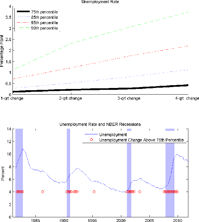
Most of the forecast combinations we consider include a forecast conditional on the unemployment rate. Figure 1 provides motivation for our interest in unemployment. The top panel shows percentile curves for the change in the unemployment rate over a horizon between 1 and 4 quarters. Remarkably, the bottom panel highlights that periods when the quarterly change in the unemployment rate is above the 75th percentile can pick up NBER recessions well ahead of the official NBER announcements.
3 Results
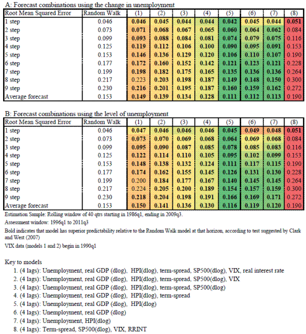
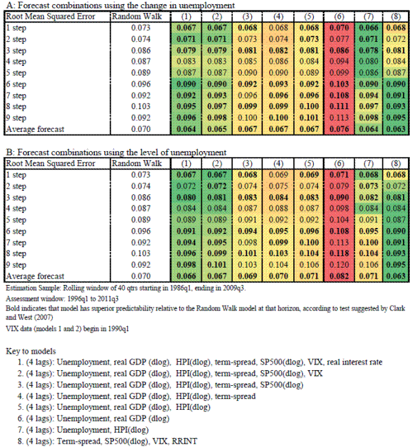
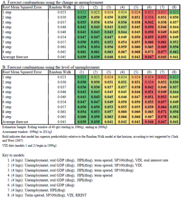
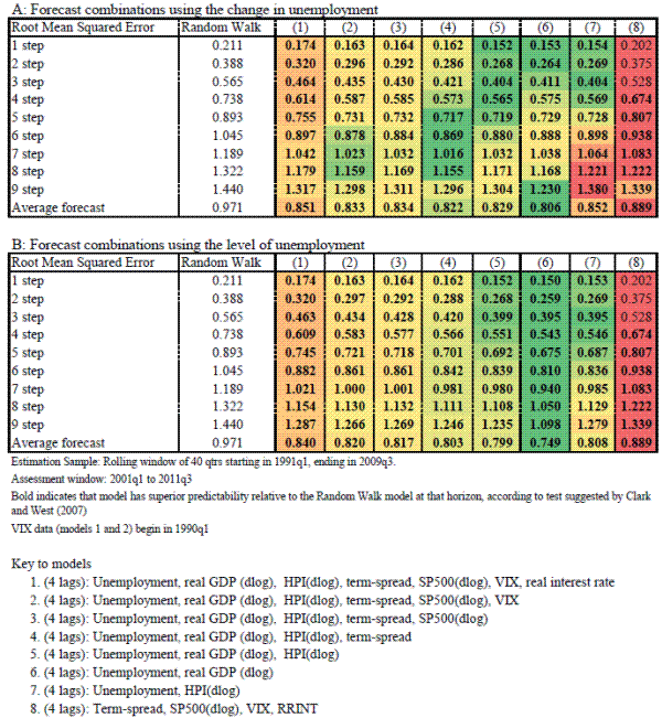
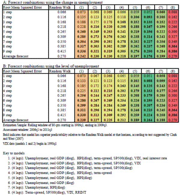
Figures 2 to 5 allow a comparison of the RMSEs for different combinations of simple models with each figure focusing on a different measure of banking conditions. We consider eight different models. Model 1, the broadest, is a combination of forecasts conditional on two groups of variables, the macro group and the financial group. Model 5 only includes the macro group, while models 2 to 4 are intermediate models that eliminate one of the financial variables at a time. Model 6 and 7 pare down the macro variables. Finally, model 8 considers the performance of a forecast combination that includes only the financial group. Each figure shows two sets of results - we alternatively include the level or the change of the unemployment rate. In each figure we use a color scheme to facilitate the comparison of results. The lowest RMSEs at each horizon are shown against a deep green background, and the highest RMSEs are shown against a red background. Shades from green to orange are used for intermediate results.
We determine when macro variables improve upon the random walk forecast using the test of Clark and West (2007). Under the null hypothesis, the random walk model is the data-generating process. Then parameters that are zero in population are correctly set to zero in sample, implying a gain in efficiency. Conversely, the alternative model introduces noise into the forecasting process that inflates its RMSE in sample. Accordingly, Clark and West (2007) recommend a downward adjustment of the sample RMSE for the alternative hypothesis. Thus, it is possible to reject the null of equal predictive ability even when, in sample, the RMSE of the alternative hypothesis is higher than the RMSE of the random walk model.
We use a one sided test. In the tables, the RMSEs for which we reject the null of equal predictive ability at the 5% significance level are highlighted in bold face.
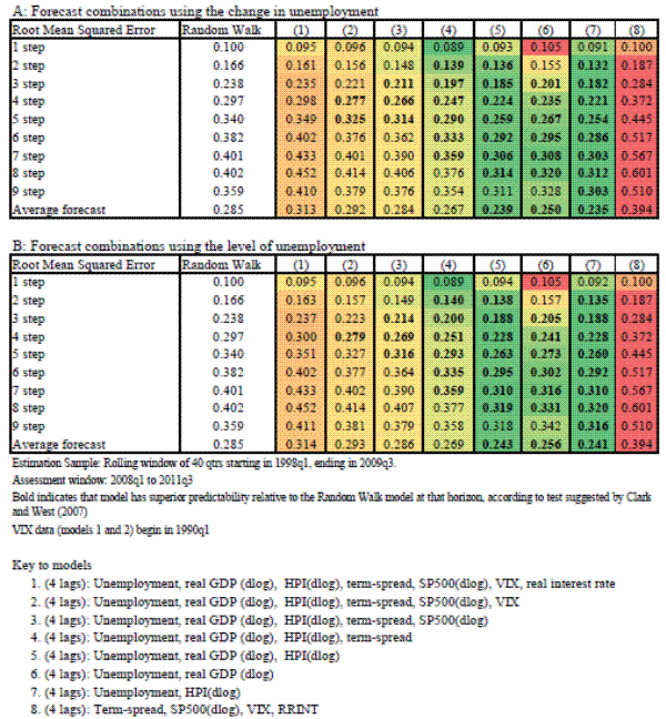
Figure 2 focuses on results for total net chargeoffs. Model 5, with the change in unemployment, real GDP, and HPI has the lowest RMSE at all horizons and beats a random walk also at all horizons. Models 6 and 7, both include unemployment, but drop HPI and GDP in turn. In both cases, the combination forecast still beats a random walk forecast, based on RMSE, if a bit more modestly. In particular, HPI seems to help at reducing the RMSE at the shorter forecast horizons.
These three models are consistent with the hypothesis that sudden changes in unemployment can reduce the ability of borrowers to repay their loans, resulting in substantial increases in chargeoffs. By contrast, the combination of models that includes financial variables only (model 8) has the worst performance in terms of RMSE - well above a random walk. Moreover, the figure shows that inclusion of the financial variables substantially worsens the forecast performance.
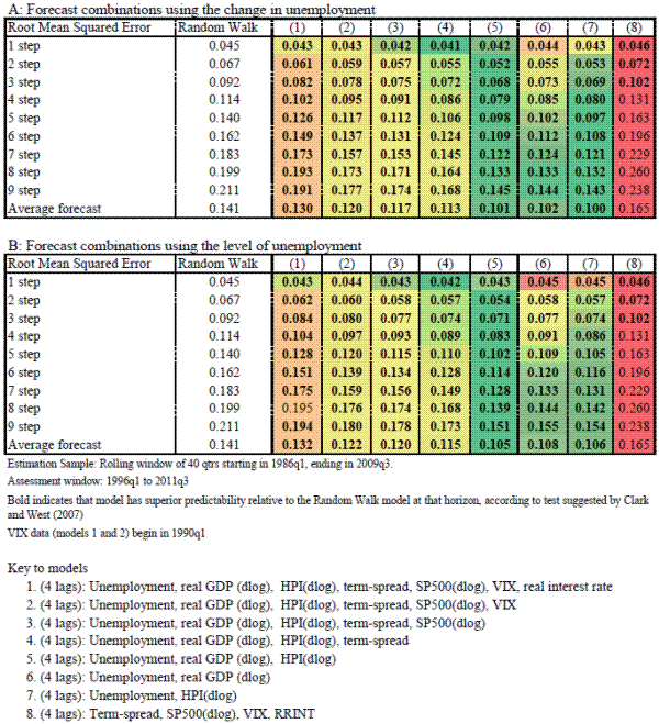
Figures 3 and 4 show results for our revenue measures, respectively PPNR and NIM. In this case, the broadest model, Model 1, performs best in terms of RMSE. Model 8, which had the highest RMSE for total net chargeoffs, displays a relatively good performance for PPNR and NIM. Overall, however, even the best-peforming models show more modest gains relative to a random walk than in the case of total net chargeoffs. In the case of PPNR, even the best performing model does not beat a random walk at all horizons.
Figure 5 focuses on tier-1 capital. Model 6, with the level of unemployment and GDP displays the lowest RMSE and beats the random walk forecast at all horizons. With the tier-1 capital ratio, the forecast combination that has the worst performance includes financial variables only.
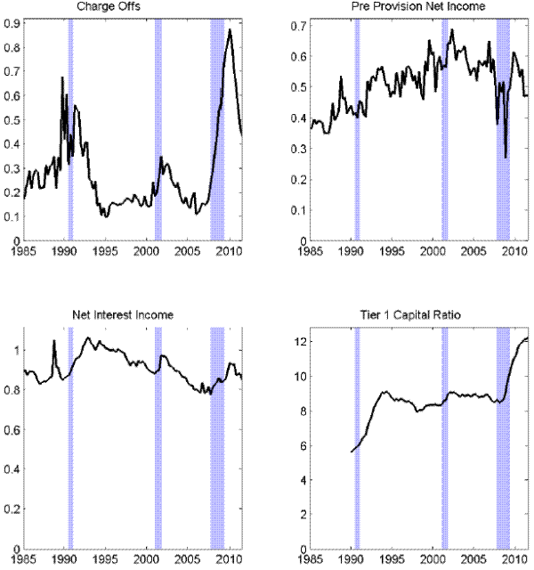
Overall, we were not able to beat a random walk across all horizons for all of the measures of banking conditions that we considered. The relative gains in RMSE were most pronounced for chargeoffs and modest for NIM and tier-1 capital. Figure 6 shows the banking measures considered against the NBER recession dates. Total net chargeoffs show clear procyclicality. NIM and the tier-1 capital ratio, while much less volatile, also show some increases in recessions. By contrast, pre-provision net income does not follow one pattern across the three recessions spanned by the data available. For instance, in the most recent recessions, pre-provision net income shows multiple peaks and troughs.
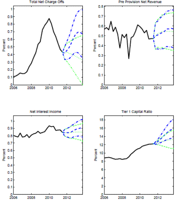
Even when the forecast combination outperformed the random walk forecast, the best performing models we could formulate were still saddled with a substantial degree of forecast uncertainty. As an example, Figure 7 shows forecasts for each of the measures of banking conditions considered. The estimation sample ends in 2009Q2, leaving 9 quarters for the assessment window till the end of our sample in 2011Q3.
Even when we do beat a random walk, the forecast uncertainty bands in Figure 7 imply a striking degree of uncertainty for each point forecast at different horizons even when compared to the abnormal variation observed in each series coinciding with the recent financial crisis. While we cannot claim to have formulated the most efficient forecast model possible for each of the measures of banking conditions considered, we interpret our results as a cautionary factor in the analysis of capital plans produced by bank holding companies as part of a stress test exercise.
3.1 Sensitivity Analysis
We perform sensitivity analysis regarding several dimensions of the benchmark forecast exercise. To verify that aggregation of data for commercial banks in the Call Report dataset to the level of Bank Holding Company did not skew the benchmark results, we use alternative data from form FR-Y9C filings that does not require aggregation. Furthermore, we forecast alternative aggregate measures for the universe of U.S. commercial banks, instead of focusing on the largest U.S. bank holding companies. We consider a shorter sample that ends before the recent financial crisis. Finally, we consider sensitivity to alternative choices for the size of the estimation window - in turn 60, or 80 quarters, instead of 40 quarters in the benchmark results. In all cases, to conserve space, we focus on chargeoffs on loans and leases and do not report sensitivity results for the additional measures of banking conditions considered above.
Figure 8 shows results for the Form Y9C dataset.8 Figure 9 shows results for an aggregate measure of chargeoffs for all U.S. commercial banks using Call Report data. In both cases, model number 5 with unemployment, GDP, and HPI all in differences remains the best performing forecast combination and the model that includes all the variables in our financial group the worst. Moreover, the performance of the best model still beats that of the random walk model in terms of lower RMSE. We conclude that neither the aggregation procedure to bank holding company in the Call Report dataset, nor consideration of the top 25 bank holding companies only skews our benchmark results.
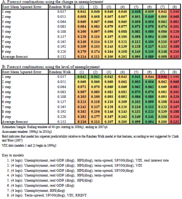
Figure 10 shows RMSEs based on a sample of data and assessment window that stop before the recent financial crisis. The last 40-quarter estimation sample considered ends in 2005Q3, leaving 9 quarters for the last assessment window spanning from 2005Q4 to 2007Q4. Even the best forecast combination model - still model 5 - fails to beat a random walk in terms of RMSE at all of the horizons considered. The deterioration in performance is more marked for model number 7, that includes only the unemployment rate and HPI. We conclude that the inclusion of HPI brings about an important improvement in performance of the forecast combination especially when considering a sample that includes the recent financial crisis.
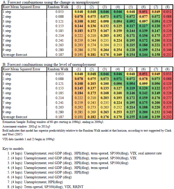
Finally figures 11 and 12 show results for a rolling estimation sample of 60 and 80 quarters, respectively, instead of 40 quarters in the benchmark. We conclude that the main results in the benchmark experiment continue to hold with these alternative estimation windows.
3.2 Sensitivity of Forecasts conditional on CCAR macro scenarios
In this section we return to the original motivation for our forecast comparisons, the application to macro stress testing. We generate forecasts of our four measures of banking conditions conditional on the macro scenarios included in the most recent stress test for bank holding companies conducted by the Federal Reserve, CCAR 2012. Two scenarios were included, a baseline scenario, and a severe stress scenario. The stress scenario is meant to represent "highly adverse conditions", while the baseline is meant to capture "expected economic conditions."9 Considering both scenarios allows us to assess the relative sensitivity of the banking conditions forecasts to the baseline and stress CCAR scenarios.
To construct the forecasts conditional on CCAR scenarios, the estimation sample ends in 2011q3. Each CCAR scenario includes all the macro variables needed by the alternative models considered in the previous sections. The scenarios extend 13 quarters out. The forecasts we present stop 9 quarters out, as the bank holding companies in the stress test are only required to produce capital plans for the next 9 quarters.
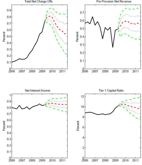
Figure 13 shows dynamic forecasts conditional on either the stress scenario or the baseline scenario for each of the measures of banking conditions considered. For each measure we selected the best performing model out of the 8 models assessed above.10 The figure also shows a 2-RMSE uncertainty band centered around each forecast.
One of the striking features that emerge from Figure 13 is that the uncertainty bands for the baseline scenario encompass the point forecasts conditional on the stress scenarios. Only in the case of total net chargeoffs and tier-1 capital ratio do the point forecast veer outside of the uncertainty bands towards the end of the capital planning horizon.
It is also interesting to consider the sensitivity of the point forecast to the different scenarios. The difference between the point forecasts for PPNR and NIM is modest. By contrast, for total net chargeoffs and tier-1 capital, going 9 quarters out, the difference between the point forecasts for the baseline and stress scenarios is sizable. In both cases, it is about half of the increase observed during the recent financial crisis. However, notice that Tier-1 capital is predicted to increase in a severe recession. This is in accordance with the pattern observed in the data. As shown in Figure 6, the tier-1 capital ratio increased during each of the three recessions for which we have data from the Call Report dataset.
4 Conclusion
This paper contributes to the empirical underpinnings of stress test exercises. For some but not all measures of aggregate banking conditions, forecasts conditional on macro variables outperform random walk forecasts in terms of root mean squared errors. The largest gains are for total chargeoffs on loans and leases. We found relatively more modest gains for net interest income and the tier-1 capital ratio. However, even our best performing model did not beat a random walk at all horizons for Pre Provision Net Income.
Regardless of the gains, we find large RMSEs for the forecasts of all the measures of banking conditions. The RMSEs are large even when compared to the large and abnormal variation for each of the series during the recent financial crisis.
When we apply our preferred forecast models to macro scenarios used in most recent stress test conducted by the Federal Reserve, CCAR 2012, we find little sensitivity of the banking measures to scenarios that are meant to capture large macroeconomic differences. In all cases, for most of 9-quarter forecast horizon, the point estimates for the stress scenario are inside the 2-RMSE uncertainty bands around the forecast conditional on the baseline scenario.
We cannot claim to have formulated the most efficient forecast model possible for each of the measures of banking performance considered. Indeed, we have used only publicly available data, while regulators and each bank holding company have access to a greater wealth of information. Nonetheless, we interpret our results as a cautionary factor in the analysis of capital plans produced by bank holding companies as part of a stress test exercise. At the very least, our results highlight that regulators may find it difficult to explain their judgment of different bank holding companies to outside observers by relying exclusively on public data.
Operations Research Quarterly 20, 451-68.
Journal of the Operations Research Society 60(12), 1699-1707.
IMF Working Paper, 1.
Bank of England Financial Stability Review.
Journal of Econometrics 138, 291-311.
Mimeo, Federal Reserve Board.
International Journal of Forecasting 28, 145-160.
Journal of Finance 46(2), 555-576.
Review of Economics and Statistics 80(1), 45-61.
Journal of Business and Economic Statistics 146, 293-303.
OENB Financial Stability Report number 3.
Journal of Forecasting 23(6), 405-430.
 |
 |
 |
|
 |
 |
 |
 |
 |
 |