Skip to: [Printable Version (PDF)] [Bibliography] [Footnotes]

Finance and Economics Discussion Series: 2012-50 Screen Reader version ^♣

The Impact of Tax Exclusive and Inclusive Prices on Demand *

Naomi E. Feldman

Research Division

Federal Reserve Board

Bradley J. Ruffle

Department of Economics

Ben-Gurion University

August 2012

Keywords: Experimental economics, sales tax, VAT, tax salience.

Abstract:

We test the equivalence of tax-inclusive and tax-exclusive prices through a series of experiments that differ only in their handling of the tax. Subjects receive a cash budget and decide how much to keep and how much to spend on various attractively priced goods. Subjects spend significantly more when faced with tax-exclusive prices. This treatment effect is robust to different price levels, to initial shopping-cart purchases and persists throughout most of the ten rounds. A goods-level analysis, intra-round revisions as well as results from a third tax-deduction treatment all cast doubt on salience as the source of our findings.

JEL Classification: C91, H20, H31.

1 Introduction

In this paper, we test the equivalence of tax-inclusive and tax-exclusive prices with a carefully designed laboratory experiment that admits controlled variation. A series of attractive goods highly discounted in price are presented to each subject who decides how much of his cash endowment to keep and how much to spend on purchases of each good. The subject repeats this task over ten rounds with the selection of products and their prices varying over rounds. Subjects are informed either that all prices include VAT (tax-inclusive treatment or ) or that the tax will be added to all prices at the checkout (tax-exclusive treatment or ).¹ Our between-subject experimental design thus provides us with individual-level purchasing decisions under varied conditions that are systematically controlled by the experimenters.

Our main finding is that subjects in the tax-exclusive treatment spend about 30% more than those facing full tax-inclusive prices. Numerous tests of our data, and subjects in particular, reveal that subjects' decisions satisfy basic choice axioms and that subjects are equally familiar with tax-exclusive and tax-inclusive pricing. Thus, this finding cannot be dismissed as irrational purchasing behavior. We then show the robustness of the treatment effect to different price levels, to learning, to initial shopping-cart purchases and, to a lesser extent, to product category. Our observed treatment effect may be viewed as surprising in view of two central features of our experimental design that bias against any treatment difference at all. First, the experiment is repeated over ten rounds, where, after each round, subjects facing tax-exclusive pricing are shown the full tax-inclusive cost of their desired bundle. Second, subjects are able costlessly to go back and forth between the checkout and shopping screens allowing those subjects who did not initially take the tax into account to adjust their behavior within the same round.

A nascent literature on the impact of price partitioning (see, for example, Chetty, Looney and Kroft (2009), Hossain and Morgan (2006), Brown, Hossain and Morgan (2010)) provides a possible explanation for our treatment effect. These papers show that when prices are divided into multiple components, shrouding or making less "salient" certain elements of the total price results in higher purchases than would be made by clearly presenting the full price.²

While it is tempting to conclude that salience also underlies our observed treatment effect, this would be premature because alternative explanations are potentially consistent with both our findings and those of previous empirical studies. Thus, to further test the salience explanation, we introduce a tax-deduction () treatment in which subjects are informed that prices include VAT and that the tax will be refunded at the checkout. The pre-deduction prices are set such that the final prices of goods in are identical to those in and , thereby facilitating a clean comparison of purchasing behavior among the three treatments. To the best of our knowledge, the previous literature on salience addresses the effect of shrouding only for positive price components of the total price (like a tax or shipping and handling fee). The impact on demand of shrouding a negative price component of the total price (such as a VAT refund or other rebate or discount) has not been explored. Based upon our current state of knowledge, one would expect salience's effect to be symmetric for positive and negative price components; that is, just as individuals are inattentive and overconsume when approaching the tax-inclusive price from below, this same inattentiveness would predict that they underconsume when approaching the tax-inclusive price from above. And yet, counter to this prediction, purchases and expenditures in do not differ significantly from those in the tax-inclusive treatment. This begs the question of why the effect of price components holds in one direction but not the other. Through various robustness tests, we explore possible explanations for this asymmetry.

Finally, we subject salience to further scrutiny by contrasting its ability to predict good-price level purchases with two alternative explanations: "optimism" and a rounding heuristic. Ultimately, we conclude that none of these explanations can organize our data, at neither the treatment level nor the good-price level.

The next section reviews the related literature. Section 3 details the experimental design and procedures. The results of the and treatments are presented in section 4 and analyzed according to various subgroups. Section 5 reports several distinct tests of the internal validity of our data. In section 6, we estimate the amount of the tax internalized for each good in the treatment. Section 7 introduces a third treatment to evaluate the salience hypothesis. Learning and the persistence of treatment differences within and across rounds are evaluated in section 8. Finally, we assess whether salience, optimism or rounding can account for our findings in section 9. Section 10 concludes.

2 Literature

In a pioneering study on the impact of price partitioning, Morwitz et al. (1998) present subjects with a hypothetical scenario that describes two telephones. The price of one phone is all-inclusive ($82.90), while the price of the second phone is displayed as the base price plus a surcharge either in dollars ($69.95 plus $12.95) or in percentage terms ($69.95 plus 18.5%). Although subjects' ex post recollection of the price they saw was lower in the percentage-surcharge condition, they actually indicated that they would be slightly less likely to purchase this phone than the same phone in the dollar-surcharge condition compared to the phone in the all-inclusive condition.

More recently and more closely related to our paper, Chetty et al. (2009) conduct a natural field experiment in a grocery store to compare purchases under tax-exclusive and tax-inclusive prices. Price tags display original pre-tax prices, the amount of the sales tax and the final tax-inclusive price for a subset of three products groups. Scanner data show that their intervention reduced demand for the treated products by about 8% on average compared to two control groups: other products in same aisle and similar products sold in two nearby grocery stores.

The unnaturalness of tax-inclusive pricing in the United States (or what Chetty et al. (2009) refer to as "Hawthorne" effects) could potentially explain why individuals purchased fewer tax-inclusive goods. In particular, the large, unusual tax-inclusive tags may have deterred suspicious consumers from purchasing the treated goods. Moreover, these Hawthorne effects are present only for the tax-inclusive goods and not for the control goods.³

To the extent that Hawthorne effects are operative in our (or any other) laboratory experiment, they are present in all treatments in equal measure. Therefore, in our setup they cannot account for any differences in purchasing behavior between tax inclusive and exclusive pricing. Moreover, the setting of our experiment provides an additional advantage: Israelis are familiar with both tax inclusive and exclusive pricing schemes. While nearly all supermarket items (like those in our experiment) and other small purchases include VAT, many services and bigger-ticket items, such as computers, washing machines, automobiles and vacation packages, are usually quoted without VAT. In addition, even when posted prices include VAT, sales receipts typically break down the amount paid into a pre-VAT price and a total tax-inclusive price.⁴

Hossain and Morgan (2006) conduct a series of auctions on eBay in which they vary the relative magnitudes of the opening auction price and the shipping and handling fee. They find that bidders largely disregard shipping and handling charges. As a result, low opening auction prices and high shipping costs lead to higher final prices than when the reverse holds. Based on field experiments selling iPods on auction websites in Taiwan and Ireland, Brown, Hossain and Morgan (2010) conclude that disclosing shipping charges yields higher seller revenues than shrouding (i.e., hiding them) if shipping costs are low; whereas the reverse holds when shipping costs are high. Neither result follows from changes in the number of bidders arising from the disclosure policy.

Gabaix and Laibson (2006) show that if the fraction of uninformed consumers is sufficiently high, a symmetric equilibrium exists in which all firms choose to shroud the prices of add-on goods, even under competitive conditions. In a controlled laboratory experiment, Kalayci and Potters (2011) find that sellers who choose larger numbers of (worthless) attributes for their goods succeed in shrouding the value of their goods to consumers. Consequently, buyers make more suboptimal choices and prices are higher.

Carlin (2009) provides a theoretical rationale for empirically documented price dispersion, even for homogeneous products. Namely, when firms choose complex pricing structures, an increasing number of consumers respond rationally by remaining uninformed about industry prices. This, in turn, permits some firms to price above marginal cost. Motivated by this model, Kalayci (2011) shows that duopolists in experimental markets employ multi-part tariffs to confuse buyers and charge higher prices. Unlike these papers, our environment involves no strategic interaction and no price uncertainty, thereby simplifying subjects' choices. Instead, ours is an individual-choice experiment with exogenously given and known prices. These two features eliminate strategic considerations and focus the subject's decision on how many units of each good to buy.

A number of other papers examine issues of salience in prices and taxation. Barber et al. (2005) demonstrate empirically that the front-end loads and the demand for mutual funds (fund flows) are consistently negatively related, whereas demand is not significantly affected by less visible operating-expense fees. Finkelstein (2009) finds that highway toll rates are 20 to 40 percent higher than they would have been without electronic toll collection. Her results are consistent with the hypothesis that the decreased tax salience that resulted from switching from a collection system whereby individuals toss coins into a toll basket to an electronic system is responsible for the rise in toll rates. Colantuoni and Rojas (2012) find that the introduction of a 5.5% sales tax on soft drinks in the state of Maine in 1991 (and repealed in 2001) had no discernible impact on the sales volume of soft drinks at either the aggregate or the brand level. Because price elasticity estimates for soft drinks reveal less than perfectly inelastic demand, the authors conclude that consumers do not internalize the tax that is not part of the shelf price.

Issues of salience are also relevant to income taxes. Feldman and Katušák (2009) find that when facing a complicated income-tax system, households partially attribute changes in their average tax rates due to losing tax credits as changes in their marginal tax rates. Blumkin, Ruffle and Ganun (2012) compare experimentally subjects' labor-leisure choices under a consumption-tax regime with a theoretically equivalent income-tax regime. The authors find that labor supply is higher under the consumption tax. As a possible explanation, they cite the lack of salience of an indirect tax incurred only after subjects have decided how much to work.

Galle (2009) questions whether the apparent lack of salience of various taxes stems from rational neglect (i.e., the disutility of computing the tax outweighs the present discounted benefit) or cognitive limitations. He demonstrates that the welfare consequences and tax-policy implications differ dramatically depending on the mechanism that underlies individuals' disregard for such "hidden taxes". Our paper takes Galle's critique seriously by incorporating various features in our experimental design and a separate tax-deduction treatment in an attempt to identify the source of tax neglect.

3 Experimental Design, Procedures and Subjects

3.1 Experimental Design

In all experiments, subjects are endowed with 50 new Israeli shekels (NIS, about $15 USD) in each of the ten rounds of the experiment. Each round begins with the shopping stage in which the subject decides how much of his 50-NIS endowment to keep and how much to spend on the five consumption goods displayed. The subject may purchase as few (e.g., 0) or as many units of a particular good as he chooses, provided he does not exceed his 50-NIS budget. After deciding on the basket of goods to purchase and the amount of money to retain, the subject clicks on the shopping cart icon to proceed to the checkout stage in which he views an itemized summary of his chosen purchases. At this stage, he may confirm his basket of goods or return to the shopping stage to revise his purchases. To avoid the corner solution whereby a subject prefers to keep the cash and not spend anything, we offer all of the consumption goods at substantial discounts of 50%, 67% and 80% off their regular retail prices. Moreover, to avoid any inconvenience or transaction cost associated with acquiring the goods (e.g., travelling to a store, exchanging a voucher for the goods), we purchased all of the goods ahead of time, brought them to each session and paid subjects in goods and in cash at the end of the experiment according to their choices.

Table 1 presents the ten goods used in the experiment (five in each round) and their pre-tax, pre-discounted, retail prices in NIS.⁵ In consultation with the university store manager, we selected these particular goods because of their wide appeal to university students (our subject pool). We group the goods into three main product categories: junk food, school supplies and personal hygiene.

Each subject repeats the task of allocating his endowment between goods and cash over ten rounds. Within each round, the selection of goods and the discount rate of either 50%, 67% or 80% are held constant. But across rounds both are varied. The design is balanced in terms of the number of rounds (five) in which each of the ten goods appears. Each good appears with each of the other nine goods in at least one round and in no more than three rounds. Each of the three discount rates is applied to three rounds. To complete the ten rounds, a particular collection of five goods seen in one of the first three rounds by all subjects is repeated in one of rounds 7 to 9 with the same discount rate (different discount rates across different subjects). Thus, each subject saw the exact same round (i.e., same set of goods at the same discount rate) twice over the course of ten rounds. This duplicate round will serve as a test of the internal consistency of decision making to be reported in section 5.

To test the behavioral equivalence of tax-inclusive and tax-exclusive prices, we design three experimental treatments: tax-inclusive (, the baseline), tax-exclusive () and tax-deduction (). In , all prices include the 16% tax at both the shopping and checkout stages. In , prices do not include the tax at the shopping stage. Instead, subjects observe pre-tax prices at the time they place items in their shopping cart. Only when they proceed to the checkout is the 16% tax added to the price. The instructions make subjects aware that the VAT is to be added at the checkout stage (although we do not tell them exactly what the tax rate is).⁶ In , prices include the tax at the shopping stage, but subjects are told that the tax will be refunded at the checkout stage.⁷ The end result is that posted prices at the shopping stage are highest in - 16% higher than in - and 16% higher in than in , for a given good and discount rate. The checkout stage equalizes all final prices across the three treatments, thereby allowing us to compare cleanly the impact of excluding, of including and of deducting the sales tax from the posted price.⁸

For each price listed in Table 1, there are nine variants in the shopping stage based upon the possible combinations of the discount rates and whether the tax was included in, to be added to or deducted from the posted price. For example, the pre-tax, pre-discount rate for the chocolate bar was 5.54 NIS. Before checkout, subjects saw this price discounted to 2.78, 1.83 and 1.11 NIS in the case of the 50%, 67% or 80% discount, respectively. subjects saw 3.21, 2.12 and 1.29 NIS, while subjects saw 3.72, 2.46 and 1.50 NIS.

A number of features of our experimental design bias our results against finding differences between treatments. First, on the single page of instructions for each treatment (included in the Appendix), the relevant tax treatment appears twice, once in bold font. Second, the distinct checkout stage plainly offers subjects the option to return to the shopping stage to make changes to their basket. Thus, subjects who may have initially overlooked or incorrectly estimated the tax or discount can revise their purchases accordingly. Finally, ten repetitions enable subjects who err in earlier rounds to correct their behavior later on.

To avoid satiation with any of the goods, we pay each subject on the basis of one round randomly chosen at the end of the experiment. This random-round-payment measure induces subjects to allocate their endowment according to their true preferences. If subjects were instead paid their cumulative earnings from all rounds, they could behave strategically. For instance, they may recognize that a specific good is particularly cheap in a given round and choose to purchase all of their desired units in that round and make zero purchases of that good in all other rounds. By making it known that subjects will be paid according to one randomly selected round, we prompt them to be consistent in their preferences (subject to price variation) across rounds. Given such consistency, which we will revisit in Section 5, any demand variation across rounds can be attributed to responsiveness to changes in the absolute price levels and in the composition of available goods, both of which were balanced across all treatments.

3.2 Experimental Procedures

All experiments were conducted using software programmed in Visual Basic. Once all subjects were seated at a computer terminal, they read the instructions at their own pace on their computer screens. One of the experimenters then read aloud the common elements of the instructions. Next, each of the ten goods was held up for all subjects to see and was briefly described. Any questions were answered privately before proceeding to the experiment. At the end of the experiment, one round was randomly selected for payment. While the experimenters prepared the payments, subjects completed a post-experiment questionnaire. The entire experiment lasted at most 45 minutes. The average subject payment was 29.93 NIS in cash (approximately $8.31 USD) and a bundle of goods priced at 20.07 NIS (approximately $5.58 USD) with a retail value of 67.83 NIS (approximately $18.84 USD).

3.3 Subjects

In total, 180 student subjects from Ben-Gurion University in Israel participated in one of the three treatments. Table 2 presents summary statistics of our subject pool by treatment. From Table 2 we see that the demographic makeup of the subjects (e.g., sex, age, year in university and choice of major) is balanced between treatments. In fact, the right-most column shows that we cannot reject the null hypothesis that the three sample populations were drawn from the same distribution for any of the variables. P-values from the non-parametric, rank-sum Kruskal-Wallis test range from .17 to .73. Nevertheless, we will control for these demographics throughout most of the subsequent empirical analysis.

4 Results

Figure 1 and Table 3 provide an overview of the main outcome variables of interest for each treatment and discount rate. The top panel of the figure presents the probability density function (pdf) of total expenditures by treatment and the bottom panel presents the cumulative density function (cdf). The pdf reveals that there is a larger fraction of than subjects who spend smaller amounts (less than 20 NIS). However, this observation reverses for larger expenditures (above 30 NIS) and is especially evident for expenditures between 45 and 50 NIS: 22.3% of subject-rounds involve spending at least 45 NIS - three times the percentage of observations. The observation that subjects spend more than their counterparts is made even more evident by the cdfs: the distribution of expenditures in first-order stochastically dominates that in .

Glancing at the and columns in Table 3, the treatment effect holds not only for overall expenditures, but also for per round expenditures and quantities purchased for each distinct discount rate. Lending still further support to the observed treatment effect, the percentage of subject-rounds in which subjects saved all of their budget is higher in than in for each discount rate, whereas the reverse holds for the percentage of subject-rounds in which subjects spent their entire budget.⁹ In subsequent subsections, we will explore the statistical significance of differences in purchasing behavior between and and pursue various robustness tests by exploiting the controlled variation afforded by the experimental method. The treatment will be analyzed later to help evaluate whether the salience explanation underlies observed differences between our main treatments of interest.

4.1 Empirical Specification

We begin our analysis at the subject-good-round level where we consider both quantities purchased and total expenditure for each good in each round as outcome variables. We then aggregate to the subject-round level where the dependent variables are total quantity and total expenditure in each round. Given that we utilize a between-subject design (the treatment is fixed for each subject), the results we obtain as we aggregate the data merely reflect this aggregation; that is, the final subject-round results are five times the subject-good-round results since there are five goods available in each round. Nonetheless, we provide this aggregation to provide a clear and straightforward overall round estimate of our treatment effects.

Our baseline OLS model is as follows:

where the indexes , , and represent subject, round, and good, respectively. The dependent variable is equal to either quantity () or expenditure ().¹⁰ Our main variable of interest, , is a binary indicator equal to one if the subject faces tax-exclusive prices, and zero otherwise. The vector represents demographic variables as reported in Table 2 as well as indicators for discount rate (67% or 80% with 50% as the base). represents binary indicators for goods and represents binary indicators for rounds. Finally, the idiosyncratic error term is represented by . Standard errors are clustered by subject, taking into account the correlation in the error terms over the rounds within a subject.

Columns (1) - (3) of Table 4 present the results for quantity, columns (4) - (7) report the results for total expenditure and column (8) reports the results where the dependent variable is a binary indicator for spending 45 NIS or more (roughly hitting the budget constraint). Columns (1) - (6) are at the subject-good-round level and the remaining two columns use aggregate subject-round level data. We begin with a simple regression of the outcome variable on the indicator. We then add demographic and other previously discussed controls. Lastly, we restrict the estimation to the final five rounds of the experiment to explore whether subjects exhibit learning over the course of the ten rounds.

Across columns (1) - (3) of Table 4, we observe that subjects consistently purchase a larger quantity of goods than subjects. For example, in the simple regression of column (1), subjects purchase, on average, .512 more units per good. Moving to column (2) and adding the previously discussed controls increases this estimated coefficient to .561. Both of these results are significant at the five-percent level and represent roughly 15.5 - 31% more units purchased. If subjects completely ignored the tax, these results would imply an average price elasticity between unity and two. The difference in the number of units purchased slightly decreases to .493 and remains significant at the ten-percent level in the final five rounds, suggesting that the limited learning that occurs is insufficient to eliminate the effect. Even by the sixth round, after subjects have experienced the addition of the tax at the cash register in each of the five previous rounds, they continue to purchase significantly more units than the subjects.

Total expenditures exhibit a similar pattern in columns (4) - (6). The amount spent per good is 1.032 NIS more for subjects, increases to 1.142 NIS after adding the controls and then falls to .974 in the final five rounds. The first two estimated effects are significant at the five-percent level, while the latter estimate is significant at the ten-percent level. Column (7) of the same table presents the results aggregated over the round. subjects spent, on average, 5.706 more than TI subjects.¹¹ Finally, column (8) shows that subjects were 14.5% more likely to reach the binding budget constraint.

In a post-experiment questionnaire, we asked subjects to describe their reaction to having the tax added on at the checkout. Their options were (a) "I had forgotten and it was a surprise" (18/60 subjects); (b) "roughly what I expected" (35/60 subjects); and (c) "exactly what I expected" (7/60 subjects). We reestimate our baseline models from Table 4 using only those subjects who answered (b) or (c). The results continue to hold at roughly the same point estimates and significance levels as before (unreported but available upon request). This finding suggests that inattentiveness to the tax is not a primary driver of our main findings. Even subjects who were fully aware that the tax would be added on at the checkout phase and cognizant of its approximate magnitude consistently overconsumed relative to subjects.

Finally, we reestimate Table 4 by restricting the sample to those subjects (76% of the total sample) who, in the post-experiment questionnaire, knew the correct rate of the VAT. The results (unreported but available upon request) come out even stronger. The point estimates on are larger and significant at the 1% level even in the last five rounds. This eliminates the explanation that our treatment effect follows from subjects fully internalizing the tax but at an incorrect, lower rate.

4.2 The Treatment Effect by Various Subgroups

We augment our baseline model by interacting the indicator with the discount rate and the good category (junk food, school supplies and hygiene). We describe each in turn in the next subsection. Two effects are of particular interest here. The first is that conditional upon being in the treatment, the treatment effect may vary along some dimension of interest (e.g., discount rate). This is captured by the estimated coefficient on the interaction term and can be read directly from Table 5. The second is how and compare along this same dimension of interest. This is captured by the linear combination of the estimated coefficients on and the relevant interaction term. The linear combination of the estimated coefficients are reported in the same table.

4.2.1 Discount Rates

As previously described, we subjected the prices to three different discount rates - 50%, 67% and 80% - and varied these rates over rounds (holding constant the discount rate within a round). We interact the indicator with indicators for the 67% and 80% discount rates in order to test whether purchasing behavior differs as price levels change. The quantity and expenditure results are reported in columns (1) and (2) of Table 5, respectively. The coefficients of .855 and 1.662 on the binary indicators for the 67% () and 80% () discount rates, respectively, reveal that on the whole subjects behave sensibly: they purchase more units of goods as the discount rate increases from 50% to 67% to 80%. Column (2) shows that their expenditures also increase when discount rates are higher (alternatively, they pocket less of their available budget). Moreover, from column (1) we observe that as the discount rate increases, the average number of goods that subjects purchase relative to subjects increases but this effect is not statistically significant. Column (2), however, shows an increasing negative effect on expenditures as discount rates increase.¹² Moving to the bottom portion of the Table, the estimated coefficients from the first two columns show that for each discount rate, subjects purchase significantly more items and have higher expenditures than subjects with the exception of the discount rate for which the effect weakens for quantities (and disappears for expenditures). In sum, the effect of tax-exclusive pricing is largely robust to the price level; however, when goods are priced at 80% below their retail value, tax-exclusive and tax-inclusive prices are sufficiently similar to diminish the effect of tax-exclusive pricing.

4.2.2 Consumption Categories

As discussed above, we have ten goods that can be neatly divided into the three categories of junk food, school supplies and personal hygiene. These goods differ on many dimensions, such as price, price elasticity and frequency of purchase in everyday life. The base category is junk food, represents the school supply category and the personal hygiene category. The highly significant estimated coefficient of 1.3 on in column (3) of Table 5 indicates that subjects in purchase 1.3 units more junk food than their counterparts in . Both treatment interaction terms with and are highly significant, negative and of nearly the same magnitude as the base category, suggesting that quantities purchased of these other two categories do not differ significantly between tax treatments. Column (4) reveals that subjects in spent significantly more on junk food and on hygiene (1.8 NIS and 1.2 NIS more, respectively) than did subjects in on these same categories of goods. While the treatment effect of expenditures on school supplies is also positive, it does not differ significantly from zero. One conjecture why the treatment effect is strongest for junk food items is that these purchases are often made impulsively without much forethought. As a result, these goods tend to have higher elasticities, implying that purchases become especially tempting by lower perceived prices. Goods in the school supplies and hygiene categories tend to be consumed over a longer time horizon, purchased less frequently, and have lower elasticities on average. For these reasons, purchases are less responsive to perceived price differences.

5 Internal Validity of the Data

In this section we consider the possibility that the hitherto results reflect more basic violations of rational choice theory. To do so, we develop tests to determine whether subjects exhibit internal consistency in their choices and whether they adhere to the law of demand. Our first test of internal consistency exploits the duplicate round built into our experimental design. As noted in section 3, each subject, regardless of treatment, faces the exact same round twice over the course of the ten-round experiment. Specifically, each subject sees a given set of five goods (energy bar, chocolate, marker, pen and toothbrush) at one of the three discount rates in one of the first three rounds. The same subject again confronts this same set of goods at the same discount rate in one of rounds 7 to 9. A demanding test of consistency would require the subject to purchase the identical bundle of goods in the two duplicate rounds. However, one can imagine many reasons why a subject may change his demand between rounds 1-3 and 7-9 (for example, fatigue, growing hunger, a sudden craving for chocolate). Nevertheless, we expect such revisions to be the exception rather than the rule.

Indeed, depending on the good in question, between 54% and 73% of subjects maintain the exact same quantity purchased across the two duplicate rounds. What is more, we observe that 71.7% of energy bar, 76.8% of chocolate, 80.0% of pen, 87.2% of marker and 87.2% of toothbrush purchases in the second duplicate round are within one unit of the first duplicate round.

Next we test whether subjects exhibit preference reversals between pairs of goods. For example, do subjects prefer chocolate to toothbrushes in one round and then toothbrushes to chocolate in a subsequent round? We once again focus on our two duplicate rounds since a test comparing any other pair of rounds quickly becomes intractable.¹³ A preference reversal is registered whenever a subject reverses his ordering of quantities demanded between two goods. For example, a subject purchases three chocolate bars and one toothbrush in the first duplicate round and then one chocolate bar and two toothbrushes in the second duplicate round.¹⁴ We consider all pairs of the five goods that are offered in the duplicate rounds, thus yielding 10 possible combinations. The first row of Table 6 reveals that a total of 41 preference reversals occur in , compared to 21 in , representing 6.8% and 3.5% of subjects' pairwise decisions from the duplicate rounds. Subsequent rows of Table 6 break down the total preference reversals according to pairs of goods. The comparison of energy bars with chocolate bars, for instance, accounts for seven out of the total 41 preference reversals in and five out of 21 in .

To appreciate just how few preference reversals subjects made, let us compare the above percentage of actual preference reversals for each treatment with the percentage obtained if we assume that each subject instead randomly decides how many units of each of the five goods to purchase. To determine each subject's random quantities, we draw (without replacement) from the same subject's observed distribution of quantities purchased in the round. In other words, we randomly assign each of the subject's actual five quantities to one good. If we exhaust all possible pairwise permutations of the actual quantities within the two duplicate rounds (400 permutations in total), 27.5% and 26.1% of subjects' overall choices correspond to preference reversals in and , respectively.¹⁵ We compare the distribution of each subject's actual fraction of preference reversals with the paired distribution of each subject's fraction of expected preference reversals based on random quantities purchased. The Wilcoxon matched-pairs signed-rank test strongly rejects the equality of the two distributions at less than the one-percent level of significance in both the and treatments. In sum, subjects in both treatments display a high degree of consistency in their preference ordering of goods.

Next, we test the data for potential violations of the law of demand. In Section 4.2.1 we showed that, on average, subjects increase their overall purchases as the discount rate increases from 50% to 67% and again from 67% to 80%. We now test whether this finding holds at the individual-good level where we regress tax-inclusive prices on quantity demanded and the full set of controls separately for each good and tax treatment. In all cases the estimated coefficient on price was negative and significant at a minimum 5% level (unreported but available upon request) reflecting that, on average, subjects act sensibly at the individual-good level (as do subjects). Furthermore, we reran these same individual tax treatment-good regressions controlling for individual fixed effects. Again, the estimated coefficients on the price variable are negative and significant.

Finally, we return to our claim in sections 1 and 2 that Israelis are equally familiar with tax-inclusive and tax-exclusive pricing. To test whether our subjects indeed perceived the posting of prices with and without VAT as equally natural, we asked them in the post-experiment questionnaire to rank on a scale of 1 - 5 (where 1 represents "very strange" and 5 represents "not strange at all") particular aspects of the experiment that they may have found "strange", "weird" or "unusual." Specifically, we asked subjects in the tax-inclusive treatment to rank how unusual it was that the "prices include VAT", and similarly for subjects in the tax-exclusive treatment regarding "prices do not include VAT."¹⁶ The average rankings were 3.1 () and 2.82 (), respectively. A t-test of means and the rank-sum, non-parametric Wilcoxon-Mann-Whitney test reveal that neither these mean rankings nor the treatments' distributions of responses to this item are significantly different from one another ( and , respectively). Subjects in fact appear to be similarly comfortable with posted prices that include VAT and those that add VAT at the register.

In sum, the point of this section is to highlight that our treatment effect cannot be readily dismissed on the basis of subjects' irrationality or unfamiliarity with tax-exclusive pricing. On the contrary, our data show that subjects are equally well acquainted with tax-exclusive and tax-inclusive pricing and that their choices satisfy certain criteria of sensible purchasing behavior.

6 Tax Internalization

The results thus far have established that, on average, subjects facing the tax-exclusive price purchase significantly more units and spend more than those facing the tax-inclusive price. In this section we seek to provide an estimate of how much of the tax is internalized by those facing the tax-exclusive price. Does the average subject completely ignore the tax or does he incorporate some fraction of the tax into his final price calculations? Another way to put it is that some subjects may completely ignore the tax when making their purchasing decisions, while others may fully incorporate the tax such that the effect is a weighted average of the two types in the population. We take a straightforward approach that exploits the fact that the tax is equal to a fixed percentage throughout the entire experiment. Consider the following estimable equation:

where represents the "shopping cart price" that is equal to for the treatment and for the treatment. In this specification, we treat the price as endogenous. Thus, conditional upon the quantity chosen, each subject has a predicted or perceived price.¹⁷ For the baseline treatment, there is no uncertainty about the final price and differences between actual tax-inclusive prices and predicted prices simply represent measurement error. However, for the treatment, we are left to estimate the perceived price used to make consumption decisions. Assuming that and subjects face identical demand curves for each good, when the tax is completely ignored by subjects, the estimated coefficient on the indicator should exactly equal the negative of the log of , which, in our case, equals .¹⁸

We estimate equation (2) separately for each of the goods. The results are reported graphically in Figure 2. For each good, the black horizontal bar represents the estimated amount internalized and the vertical boxes represent the 95% confidence intervals. For example, for the chocolate bar, only 2.3 percentage points on average out of the 16 (the amount of the VAT) were internalized. In other words, only a small fraction of the total tax was taken into account when calculating final prices. Another way to interpret this result is that 15% of subjects internalized the tax (equal to ) while the remaining 85% completely ignored it when making purchasing decisions. Given that zero is included in the confidence interval, we cannot reject that subjects completely ignored the tax. As the figure shows, the level of internalization varies over the goods, ranging from -.001 (completely ignoring the tax) to .138 (near full internalization).¹⁹ We test for a correlation between the ranking of the goods' point estimates of the amount of tax internalized and the goods' price levels, elasticities and other dimensions. Spearman non-parametric rank correlation tests reveal that none of these correlations are significant at traditional levels.

The average amount internalized over all goods is five percentage points; that is, roughly one-third of the subjects completely ignore the inclusion of the tax when making their purchasing decisions and the remaining two-thirds fully internalize the after-tax price (or, roughly one-third of the tax is ignored by the average subject).²⁰ However, with only two exceptions (energy bar and handcream), we cannot reject at a five-percent level of significance that the tax was completely ignored in all cases. Moreover, this finding is practically unchanged if we consider only the final five rounds (unreported but available upon request).²¹

7 Tax-Deduction Treatment

As discussed in the Introduction, salience refers to the increased visibility of certain characteristics of a good (the price in our case) and the reduced visibility of others. To the best of our knowledge, experimental tests of salience have compared only tax-exclusive (or shipping-expense-exclusive) prices to those that include the tax. A third tax-deduction treatment () furnishes us with an alternative test of salience. We take advantage of the fact that the opposite experiment of can be readily conducted in the laboratory, namely, a higher price is posted during the shopping phase and the tax is deducted from the price at the checkout. The salience hypothesis in predicts that subjects will purchase too little if they do not fully internalize the less visible discount offered at the checkout.

As in , the treatment is comprised of a final total price that is broken down into two parts - a highly visible part and a less visible part (a deduction). For example, consider the tax-inclusive price of 1 NIS. We first imposed an additional 16% tax for a shopping cart price of 1.16 NIS. Subjects see this price and are then informed that they will receive a VAT refund upon reaching the checkout. Hence, the subject observes the 1.16 NIS price and (in theory) computes the VAT deduction, arriving at a final price of 1 NIS. Thus, subjects in the treatment approach the tax-inclusive price from below, while those in the treatment approach the tax-inclusive price from above.

Recall that expenditures in first-order stochastically dominate those in . A glance at Figure 1 reveals that no such clear-cut relationship exists between and . In fact, Table 3 shows quite pointedly the likeness of and . Explicitly, these treatments are similar to one another for all of the reported measures: quantity purchased, expenditures, the fraction of rounds in which the entire budget was saved and was spent, both overall and for each separate discount rate.

To compare statistically the three tax treatments, we update equation (1) from Table 4 with an additional binary indicator, , that equals one if the subject participated in the treatment and zero otherwise. Results are reported in Table 7. The baseline continues to be the treatment. The effect of the treatment is little changed with the addition of the new treatment (as expected given that these treatments are independent). Consider next the second row of the table. Contrary to what salience would predict, subjects show no statistically significant difference in purchasing decisions from subjects. The point estimates on are much smaller overall than those on ; they vary between positive and negative signs and they are not significant at any conventional level of significance. We conclude that we cannot reject the null that on average subjects completely internalize the tax discount.

These results raise a thought-provoking question. If we view the issue of salience as "shrouded attributes," why does it work in only one direction? That is, why, on average, do subjects appear not to internalize fully a tax but yet have little difficulty doing so for a discount? One potential answer is that the ubiquity of taxes have so habituated individuals to sales taxes that they are an accepted and, ultimately, ignored part of the price. Tax rebates, on the other hand, are rarer and consequently make more of an impression upon the individual. As a result, the attentive subject accurately calculates the post-deduction, final price. This contrast in perception between taxes and discounts suggests the role of the framing of price components as a fruitful direction for future research.

8 Learning and Further Robustness Checks

As previously mentioned, two attributes of our experiment bias us against finding any treatment effect: the repetition of the experiment for ten rounds and the ability to revise the cart by moving costlessly between the checkout and shopping phases of the experiment. In this section, we further investigate how these two features of our experimental design impact our main findings.

8.1 Treatment Effect by Round

To the best of our knowledge, the current literature is agnostic about the effect of salience in a dynamic environment that grants opportunities for learning. Our experiment features ten budget allocation decisions for each individual. In fact, our design yields ten separate estimates of our treatment effect, one for each round. If higher purchases in are driven by initial inattentiveness to the addition of the tax at the checkout, then ten full repetitions of the experiment and the option to go back and forth between the checkout and cart in each round as many times as the subject pleases provide subjects with ample opportunities to correct their early inattentiveness. To illustrate these opportunities for learning, suppose in the first round a subject, oblivious to the tax, spends 20 NIS in the first shopping stage, expecting to pocket 30 NIS. Upon reaching the checkout the subject ought to be surprised to see that his purchases cost 23.6 NIS, leaving only 26.4 NIS in change. The subject can promptly return to the shopping stage to remove items from his cart. Even if the subject cannot be bothered to return, we would at least expect him to revise downward his purchases in future rounds. The round-level results are presented in Figure 3 where we run the full models from columns (2) and (5) of Table 7.

Panel (a) displays the estimated coefficients for and for the dependent variable of quantity per good and Panel (b) displays the analogous graph for the dependent variable of expenditure per good. Both are relative to . The black horizontal bars represent the point estimates and the vertical bars the 90% confidence intervals.²² Consider first Panel (a). The estimated coefficient on does not show any clear downward trend over the ten rounds, although four of the last six rounds of the experiment (5, 7, 8 and 10) are not significant at even the 10% level.²³ Three of these rounds (5, 7 and 10) also have much smaller point estimates (in the range .21 - .26) than other rounds. Some subjects appear to learn as they gain experience in the experiment. Still, the figure does not decidedly attest to a learning effect. , on the other hand, presents a thoroughly consistent picture across rounds. The point estimates are relatively small, cycle between positive and negative and, from the outset, are never significantly different from zero at even the 10% level.

Turning to Panel (b), expenditures paint a similar picture for but round 8 is now significant at the 10% level; rounds 5, 7 and 10 continue not to be. As with quantity, expenditures show a lack of significance across all ten rounds. In brief, the treatment effect for subjects shows some signs of weakening in later rounds but does not disappear altogether. subjects consistently internalize the VAT discount.

8.2 Revisits to the Shopping Cart

The laboratory offers the researcher a unique opportunity to observe not only individuals' final purchasing decisions, but also to track whether and how they revised their purchases before arriving at their final bundle. In our experiment, after reaching the checkout stage, subjects have the option of returning to their shopping cart and, if they so choose, to revise their purchases. For each time the subject reached the checkout screen, we collected total round-level expenditure. If a subject initially exceeded his 50-NIS, tax-inclusive budget, he was forced to return to his basket to remove one or more items. Others may voluntarily return to their baskets out of curiosity or after having second thoughts. Nothing in the instructions or in the software prevents subjects from toggling between the two screens as many times as they desire.

Initial purchasing decisions may reflect instinctive choices that were not weighed carefully. Initial choices are of interest because they likely parallel some settings outside the laboratory in which purchases are made under hectic conditions less conducive to the concentration afforded by sitting comfortably in front of a computer in a quiet laboratory with no time pressure. In addition, if changing one's mind involves non-negligible transaction costs (e.g., commissions, rebooking fees), then one's initial choice may become the de facto final decision that goes against one's better judgement.

Among the 180 subjects, each of whom participated in 10 rounds (for a total of 1800 subject-rounds), 81 subjects in a total of 225 rounds returned to their carts. Fifty-two of these 225 returns were imposed due to having exceeded budget.²⁴ Of the remaining 173 voluntary returns, 101 were by subjects, 28 by subjects and 44 by subjects. Conditional upon returning to their cart, about 65% returned at most twice. Only two subjects returned to their cart in every single round.

Table 8 explores these returns in more detail. The first column of the Table repeats our baseline expenditure result from Table 7 for ease of comparison. We then estimate the same model replacing the final checkout amount with the initial checkout amount. Column (2) shows that the estimated treatment effect for subjects increases slightly to 6.10 NIS and is statistically significant at nearly the one-percent level. This larger coefficient is consistent with the desire of many subjects to spend even more; but the budget constraint forces them to curtail their initial purchases. subjects, by contrast, continue to show no statistically significant difference from subjects.

Next we restrict the sample to exclude rounds up to and including a subject's first return attempt.²⁵ The idea is that up to and including a typical subject's first return he grapples most with his allocation decision. After a return to the cart we would expect subjects to better internalize (at least weakly) the tax or deduction and make decisions more automatically in subsequent rounds. The results from column (3) again reveal that on average subjects purchase more than subjects with a point estimate similar to the baseline result. This finding strengthens the round-level results that demonstrate that opportunities to learn about the tax do not eliminate the treatment effect. Here too, even after subjects are over the steepest portion of their learning curves, subjects continue to over-purchase.

9 Rounding, Salience and Optimism

The precise definition of salience remains elusive in the current literature in which salience has served as a catch-all phrase, alternately referring to ignoring the tax, putting less weight on the tax or using a simple rounding heuristic. We now put more structure on the definition while at the same time we differentiate inattentiveness from rounding. We refer to salience as ignoring or underestimating the less visible price element. Salience implies that the perceived tax-inclusive price will always be lower than the true tax-inclusive price. Rounding, by contrast, invokes a particular heuristic to approximate the tax-inclusive price and may yield higher or lower prices than the true tax-inclusive price.

In addition to rounding, we propose "optimism" as a second alternative hypothesis to salience. Like rounding, optimism implies that individuals are aware of the tax and perhaps even the precise tax rate, but err in determining the final tax-inclusive price. An individual who manifests an optimism bias systematically underestimates the magnitude of the tax to be paid in order to reduce the cognitive dissonance associated with purchasing at a higher price or, more generally, in order to justify the purchase to himself. The flip side of optimism is that individuals overestimate discounts in order to derive psychological satisfaction from paying a lower price.

A rounding heuristic may be employed to reduce the cognitive effort required to compute each and every tax-inclusive price. One intuitive method of rounding involves rounding up tax-exclusive prices to the nearest whole monetary unit. For sufficiently low-priced goods, like those used in our experiment, such a rule of thumb yields an overestimate of the tax-inclusive price as often as an underestimate. Rounding implies that consumers approximate the final price and base their consumption decisions on the approximated price. How to round is not uniquely defined and we will consider two heuristics: to the nearest shekel and to the nearest half shekel.²⁶

Since none of our tax-inclusive prices happen to be whole numbers exactly 16% above (below) the tax-exclusive (tax-deduction) price, rounding always leads to a price different from the actual price in . For a given demand curve of each good, this price discrepancy implies that subjects on average purchase different quantities of the same good in the two treatments. For example, at a 50% discount rate on handcream, subjects observe a tax-exclusive price of 6.28. According to the nearest-shekel rounding heuristic, they round up this price to 7 and base their purchasing decisions on this rounded price. Because subjects see a higher price of 7.28 for handcream, this rounding heuristic predicts that subjects will over-purchase, on average. On the other hand, this same handcream, when discounted at a rate of 67%, yields an observed price of 4.14 for subjects. When rounded up to 5, the price exceeds the true price of 4.81 in , implying that on average subjects will under-purchase.

In the treatment, the nearest-shekel rounding heuristic suggests that subjects round down to the nearest shekel. With the same 30 combinations of goods and discount rates in each treatment, the rounding explanation yields 30 directional hypotheses in purchasing behavior between and and another 30 between and . Each directional hypothesis follows from a price difference between the treatment under consideration ( or ) and for a given good and discount rate.

Consider the top row of Table 9. The first cell shows that when rounding to the nearest shekel, 14 (out of 30) perceived prices are lower than the true, tax-inclusive price. For these 14 cases, we predict that subjects purchase more than subjects. Because average purchases have an associated standard error, we bootstrap the procedure to calculate the number of times that our prediction is true. The endpoints of a 95% confidence interval (percentile) show that 10 - 14 out of 14 cases have subjects purchasing more than subjects. One-sided Binomial tests reveal that the probability that these proportions (10/14 and 14/14) could be generated by a random process (with an expected proportion of 7/14) is equal to .090 and .000, respectively. Thus, we reject this outcome as random in favor of the alternative hypothesis of rounding. The next cell in the same row shows that the remaining 16 rounded prices are higher than the true, tax-inclusive case. In these cases, we predict that on average subjects purchase less than subjects. The 95% confidence interval shows a range of two to seven cases have subjects purchasing less than subjects. Thus, we cannot reject the null that this is random in favor of the alternative rounding hypothesis (p-values of .773 and .999).

Continuing along the same row, when comparing purchasing behavior in and , we cannot reject that the observed fraction of outcomes differs from chance, neither when the rounded down price is less than the actual price (95% confidence interval endpoint p-values of .032 and .676) nor when it exceeds the price (95% confidence interval endpoint p-values of .113 and .887). We also consider an alternative rounding heuristic whereby subjects round up () or down () to the nearest half shekel.²⁷ Overall, the results from Table 9 reveal limited support for both forms of rounding. Only the first column (when the rounded price is below the actual price) shows support for rounding in both forms. In all other cases, we cannot reject the hypothesis that the indicated fraction of outcomes consistent with rounding differs from chance in favor of rounding at any conventional level of significance.

Regardless of whether subjects entirely or only partially ignore the tax or deduction, salience always leads to lower perceived prices in compared to the same good-discount rate combination in . Similarly, an optimism bias also yields perceived prices in below those in . In both cases subjects should purchase more. The endpoints of the 95% confidence interval are 20 - 27 with corresponding p-values equal to .049 and .000. We reject the null hypothesis in favor of the alternative in both cases. As previously discussed, salience and optimism part ways in the relationship between perceived prices in compared to . Confirming the regression results of the previous section, the right-hand columns of Table 9 indicate that neither salience (10 - 17 cases) nor optimism (13 - 20 cases) garners much support in explaining purchases in relative to . While the p-values are somewhat smaller for optimism (.049 - .889) compared to salience (.292 - .987), their range is sufficiently wide such that we do not confidently reject the null hypothesis of random average quantities purchased in favor of optimism.

Overall, none of the mechanisms described in this section adequately organize our data.²⁸ When perceived prices are below those of , then all three mechanisms are plausible. Things fall apart, however, for perceived prices above prices and for perceived prices both above and below prices. It may very well be that some segments of the population are optimistic while others are inattentive such that no one theory dominates.

10 Conclusions

In the broadest sense, our experiment tests for a tax-framing effect on consumer demand: three identical environments differ merely in the way the price is initially presented to subjects. The tax frame ought not to matter since the products' final prices are identical across treatments. And yet consistent with recent literature showing that not all price components are treated equally, we too find differences in consumer demand across tax treatments. Most importantly, subjects buy more under a tax-exclusive regime than under an equivalent tax-inclusive regime.

Using the rich data set that we generated from the lab, we explore further this empirical finding. Despite ten rounds of choice in this full-information environment with feedback at the end of each round, the treatment effect persists throughout the experiment, albeit weakens in the final rounds. Learning appears limited. Moreover, even the ability to revise freely the desired bundle after seeing the tax-inclusive price does not eliminate the effect. The effect is also robust to changing price levels, different compositions of goods and, to a lesser degree, the category of good. Junk food items are especially susceptible to the treatment effect, perhaps because demand for these goods is rather elastic and purchases of them are often made impulsively. Impulsiveness combined with a lower perceived price in the tax-exclusive treatment induce subjects to consistently overbuy. We estimate that subjects in the tax-exclusive treatment internalize only five percentage points or roughly one-third of the 16% tax on average across all goods. For eight out of ten individual goods, we cannot reject the hypothesis that subjects ignore the tax entirely. To investigate the source of our treatment effect, we introduce a third treatment in which a price component (the tax) is subtracted from the final price. Quantities and expenditures in this tax-deduction treatment do not differ significantly from those in the tax-inclusive treatment. The results from this treatment, an analysis of purchases at the good-price level as well as insights from intra-round revisions to purchases all suggest that salience may not be the key explanation for the finding in the literature that price partitioning leads to differences in consumption.

The short-run policy implications are manifold. First, to raise a given amount of tax revenue, the required tax rate is lower for tax-exclusive pricing than for tax-inclusive pricing. The reason is that consumers adjust their behavior less under a tax-exclusive regime, thus resulting in a more efficient second-best outcome.²⁹ Second, given that a tax is not fully internalized, the government can choose between a VAT or sales-tax style tax based upon whether it aims to discourage a taxed activity. For example, sin taxes or taxes on goods that impose a negative externality are best implemented with a VAT whereas taxes on goods that are complementary with labor are best implemented with a sales tax. Third, switching from a VAT to a sales-tax regime during an economic downturn may provide short-term stimulus to the economy in the form of increased consumption, government revenues and producer welfare.³⁰ The long run is less clear. On the one hand, the lack of internalization allows a greater proportion of the tax to be shifted onto the consumer. Producers benefit as the after-tax price they receive is higher, as is demand. On the other hand, our experiment suggests that, over time, the impact of any government manipulation of how the tax is imposed may become less effective, though not disappear entirely.

References

Bibliography

Anderson, Eric T. and Duncan I. Simester (2003) "Effects of $9 Price Endings on Retail Sales: Evidence from Field Experiments," Quantitative Marketing and Economics, 1, 93-110.

Barber, Brad, Terrance Odean and Lu Zheng (2005) "Out of Sight, Out of Mind: The Effects of Expenses on Mutual Fund Flows," Journal of Business, 78, 2095-2119.

Blumkin, Tomer, Bradley J. Ruffle and Yosef Ganun (2012) "Are Income and Consumption Taxes Ever Really Equivalent? Evidence from a Real-Effort Experiment with Real Goods," European Economic Review, 56, 1200-1219.

Brown, Jennifer, Tanjim Hossain and John Morgan (2010) "Shrouded Attributes and Information Suppression," Quarterly Journal of Economics, 125:2, 859-876.

Carlin, Bruce I. (2009) "Strategic price complexity in retail financial markets," Journal of Financial Economics, 91, 278-287.

Chetty, Raj, Adam Looney and Kory Kroft (2009) "Salience and Taxation: Theory and Evidence," American Economic Review, 99:4, 1145-1177.

Colantuoni, Francesca and Christian Rojas (2012) "The Effect of Soft Drinks Taxes on Consumption: Evidence from Scanner Data," unpublished manuscript.

Feldman, Naomi and Peter Katušák (2009) "Effects of Predictable Tax Liability Variation on Household Labor Income," unpublished manuscript.

Finkelstein, Amy (2009) "EZ-Tax: Tax Salience and Tax Rates," Quarterly Journal of Economics, 124:3, 969-1010.

Gabaix, Xavier and David Laibson (2006) "Shrouded Attributes, Consumer Myopia, and Information Suppression in Competitive Markets," Quarterly Journal of Economics, 121:2, 505-540.

Galle, Brian (2009) "Hidden Taxes," Washington University Law Review, 87, 59-114.

Hossain, Tanjim and John Morgan (2006) "...Plus Shipping and Handling: Revenue (Non) Equivalence in Field Experiments on eBay," B.E. Press Advances in Economic Analysis & Policy, 6:2, Article 3.

Kalayci, Kenan and Jan Potters (2011) "Buyer confusion and market prices," International Journal of Industrial Organization, 29:1, 14-22.

Kalayci, Kenan (2011) "Price complexity and buyer confusion in markets," unpublished manuscript.

McCartney, Scott (2011) "Now, Even the Cheap Seats on Airplanes Come With a Fee," Wall Street Journal, November 3.

Morwitz, Vicki G., Eric A. Greenleaf and Eric J. Johnson (1998) "Divide and Prosper: Consumers' Reactions to Partitioned Prices," Journal of Marketing Research, 35:4, 453-463.

Table 1: Pre-sales tax and Pre-discount Prices of Goods in the Experiment

Junk Food Energy Bar	2.65
Junk Food Chocolate Bar	5.54
Junk Food Pack of Gum	3.70
School Supplies Highlighter	2.86
School Supplies Pen	6.80
School Supplies Pad of Paper	5.97
Hygiene Handcream	12.56
Hygiene Deodorant	17.73
Hygiene Toothbrush	5.03
Hygiene Toothpaste	13.36

Notes: Retail prices (not including the sales tax) in New Israeli Shekels (1 USD = 3.6 NIS) for each of the ten goods used in the experiment.

Table 2: Socio-Demographic Summary Statistics

Treatment	TE	TI	TD	Kruskal-Wallis test
Variable	Mean(Std. Dev.)	Mean(Std. Dev.)	Mean(Std. Dev.)	p-value
Male	.500	.450	.550	0.90
Male (Standard Error)	(.500)	(.498)	(.498)	.64
Age	25.32	24.93	25.03	1.35
Age (Standard Error)	(1.68)	(1.75)	(3.33)	.51
Undergrad	.900	.967	.983	0.70
Undergrad (Standard Error)	(.302)	(.181)	(.128)	.71
Economics Major	.150	.183	.233	0.63
Economics Major (Standard Error)	(.357)	(.387)	(.423)	.73
Engineering Major	.617	.517	.417	3.58
Engineering Major (Standard Error)	(.486)	(.500)	(.493)	.17
Other Major	.233	.300	.350	1.23
Other Major (Standard Error)	(.423)	(.458)	(.477)	.54
Obs. (Subjects)	60	60	60	60

Notes: The last column reports the results of non-parametric, rank-sum Kruskal-Wallis tests comparing the three treatments for each of the variables.

Table 3: Round-Level Summary Statistics of Outcome Variables

	Treatment	TE	TI	TD
Discount Rate	Variable	Mean (Std. Dev.)	Mean (Std. Dev.)	Mean (Std. Dev.)
0.5	Quantity of Goods Purchased	6.00	3.89	3.80
0.5	Quantity of Goods Purchased (Std. Dev)	(5.48)	(4.34)	(4.09)
0.5	Final Expenditure	22.35	14.46	15.17
0.5	Final Expenditure (Std. Dev)	(18.94)	(15.11)	(15.87)
0.5	Spent Nothing	.193	.323	.275
0.5	Spent Nothing (Std. Dev)	(.395)	(.468)	(.447)
0.5	Spent All	.250	.067	.078
0.5	Spent All (Std. Dev)	(.434)	(.252)	(.268)
0.5	Obs.	192	192	207
0.67	Quantity of Goods Purchased	10.91	8.36	9.94
0.67	Quantity of Goods Purchased (Std. Dev)	(9.06)	(6.51)	(8.97)
0.67	Final Expenditure	22.89	18.46	18.48
0.67	Final Expenditure (Std. Dev)	(17.31)	(13.87)	(16.84)
0.67	Spent Nothing	.070	.098	.074
0.67	Spent Nothing (Std. Dev)	(.255)	(.297)	(.262)
0.67	Spent All	.201	.074	.109
0.67	Spent All (Std. Dev)	(.402)	(.263)	(.312)
0.67	Obs.	214	215	202
0.8	Quantity of Goods Purchased	15.34	12.32	12.75
0.8	Quantity of Goods Purchased (Std. Dev)	(13.56)	(9.38)	(11.41)
0.8	Final Expenditure	22.68	19.42	19.96
0.8	Final Expenditure (Std. Dev)	(17.29)	(14.03)	(15.47)
0.8	Spent Nothing	.052	.026	.037
0.8	Spent Nothing (Std. Dev)	(.221)	(.159)	(.188)
0.8	Spent All	.222	.104	.120
0.8	Spent All (Std. Dev)	(.390)	(.292)	(.293)
0.8	Obs.	194	193	191
Totals	Quantity of Goods Purchased	10.77	8.21	8.72
Totals	Quantity of Goods Purchased (Std. Dev)	(10.59)	(7.80)	(9.39)
Totals	Final Expenditure	22.65	17.50	17.81
Totals	Final Expenditure (Std. Dev)	(17.81)	(14.44)	(15.76)
Totals	Spent Nothing	.103	.147	.132
Totals	Spent Nothing (Std. Dev)	(.304)	(.354)	(.338)
Totals	Spent All	.223	.082	.102
Totals	Spent All (Std. Dev)	(.417)	(.274)	(.302)
Totals	Obs.	600	600	600

Notes: For each of the three treatments (, and ) and each of the three price discount rates (0.5, 0.67 and 0.8), the table reports the mean number of items purchased in a round and the mean amount of money spent on goods in a round. The last two rows in each panel indicate the fraction of rounds in which subjects spent none of their budget and at least 45 NIS of their budget on goods, respectively.

Table 4: The Effect of Tax-Exclusive Prices on Quantity Demanded and Expenditure

	Quantity-Good Level (1)	Quantity-Good Level (2)	Quantity-Good Level (3)	Expenditure-Good Level (4)	Expenditure-Good Level (5)	Expenditure-Good Level (6)	Expenditure-Round Level (7)	Expenditure-Round Level (8)
	.512	.561	.493	1.032	1.142	.974	5.706	.145
(standard error)	(.243) **	(.238) **	(.252) *	(.512) **	(.494) **	(.524) *	(2.485) **	(.052) ***
	1.641	2.603	2.550	3.499	1.833	1.079	13.926	.176
(standard error)	(.135) ***	(1.217) **	(1.201) **	(.291) ***	(2.720)	(2.585)	(13.788)	(.196)
	6000	6000	3000	6000	6000	3000	1200	1200
	.006	.135	.156	.007	.090	.092	.156	.134
Controls	NO	YES	YES	NO	YES	YES	YES	YES
Rounds	1-10	1-10	6-10	1-10	1-10	6-10	1-10	1-10

Notes: Controls include demographics (Table 1), round, good and discount rate indicators. Columns 7 - 8 exclude good indicators. Dependent variable in column 8 is a binary indicator for spending at least 45 NIS, zero otherwise. Standard errors clustered by subject. 10 percent significance level, ^**5 percent significance level, 1 percent significance level.

Table 5: The Effect of Tax-Exclusive Prices on Quantity Demanded and Expenditure (by Subcategory)

	Discount Rate Quantity (1)	Discount Rate Expenditure (2)	Category Quantity (3)	Category Expenditure (4)
	.430	1.616	1.309	1.800
(standard error)	(.159) ***	(.551) ***	(.487) ***	(.644) ***
	.855	.838
(standard error)	(.105) ***	(.227) ***
	1.662	1.073
(standard error)	(.150) ***	(.310) ***
	.151	-.581
(standard error)	(.156)	(.334) *
	.216	-.882
(standard error)	(.278)	(.389) **
			-.826	-.141
(standard error)			(.303) ***	(.485)
			-1.165	1.047
(standard error)			(.225) ***	(.447) **
			-1.069	-1.446
(standard error)			(.489) **	(.721) **
			-1.087	-.604
(standard error)			(.431) **	(.681)
	1.170	2.268	1.879	2.045
	.581	1.035
(standard error)	(.250) **	(.509) **
	.647	.734
(standard error)	(.364)	(.534)
			.240	.354
(standard error)			(.285)	(.558)
			.222	1.195
(standard error)			(.201)	(.709)
	6000	6000	6000	6000
	.077	.041	.13	.053

Notes: Base categories: Discount rate (50%), category (junk food). Standard errors clustered by subject.
10 percent significance level, ^**5 percent significance level, 1 percent significance level.

Table 6: Preference Reversals by Tax Treatment

	TE	TI
Total Preference Reversals	41/600 (6.8%)	21/600 (3.5%)
Energy Bar-Chocolate	7/60	5/60
Energy Bar-Marker	5/60	1/60
Energy Bar-Pen	2/60	0/60
Energy Bar-Toothbrush	2/60	0/60
Chocolate-Marker	2/60	1/60
Chocolate-Pen	7/60	3/60
Chocolate-Toothbrush	4/60	1/60
Marker-Pen	5/60	3/60
Marker-Toothbrush	2/60	4/60
Pen-Toothbrush	5/60	3/60
Total Preference Reversals based on Random Choice	6594/24000 (27.5%)	6266/24000 (26.1%)
Comparison of subject's actual and random-choice-based preference reversals: % actual % random	5/60	1/60
Comparison of subject's actual and random-choice-based preference reversals: % actual % random	5/60	7/60
Comparison of subject's actual and random-choice-based preference reversals: % actual % random	50/60	52/60
Wilcoxon matched-pairs signed-rank test

Notes: The first row indicates the total number of observed preference reversals by treatment, subsequently broken down by pairs of goods. A preference reversal between goods and is defined as follows: in the first duplicate round followed by in the second duplicate round. For comparison, the next row provides the total number of preference reversals based on the assumption that each subject chooses how many units to purchase of each good randomly from among his actual quantities. The next three rows indicate the fraction of subjects for whom their percentage of observed preference reversals is, respectively, greater than, equal to, and less than their percentage of preference reversals based on random choice. The final row reports a non-parametric test that compares the paired subject-level actual and random distributions of preference reversals.

Table 7: The Effect of Tax-Exclusive and Tax-Deduction Prices on Quantity Demanded and Expenditures

	Quantity-Good Level (1)	Quantity-Good Level (2)	Quantity-Good Level (3)	Expenditure-Good Level (4)	Expenditure-Good Level (5)	Expenditure-Good Level (6)	Expenditure-Round Level (7)	Expenditure-Round Level (8)
	.512	.560	.492	1.032	1.153	.995	5.759	.149
(Standard Error)	(.242) **	(.236) **	(.250) **	(.511) **	(.490) **	(.521) *	(2.461) **	(.052) ***
	.102	.045	-.012	.063	-.080	-.155	-.482	.006
(Standard Error)	(.214)	(.216)	(.228)	(.442)	(.448)	(.474)	(2.233)	(.039)
	1.641	3.888	3.658	3.499	3.748	2.691	21.489	.166
(Standard Error)	(.135) ***	(1.054) ***	(.980) ***	(.290) ***	(2.173) *	(1.973)	(10.771) **	(.156)
	9000	9000	4500	9000	9000	4500	1800	1800
	.004	.121	.136	.006	.077	.080	.101	.098
Controls	NO	YES	YES	NO	YES	YES	YES	YES
Rounds	1-10	1-10	6-10	1-10	1-10	6-10	1-10	1-10

Controls: Demographics (Table 1). Columns 2 - 6 include round, good, good table, and discount rate indicators. Columns 7 - 8 include round, good table, and discount rate indicators. Dependent variable in column 8 is a binary indicator for spending at least 45 NIS, zero otherwise. Standard errors clustered by subject. 10 percent significance level, ^**5 percent significance level, ^***1 percent significance level.

Table 8: The Effect of Tax-Exclusive and Tax-Deduction Prices on Round-Level Expenditures

	Final Checkout (Baseline) (1)	Initial Checkout (2)	Final Checkout (Post Return) (3)
	5.759	6.098	5.634
(standard error)	(2.462) **	(2.518) **	(2.517) **
	-.432	-.704	-.736
(standard error)	(2.247)	(2.222)	(2.260)
	21.489	21.831	23.161
(standard error)	(10.771) **	(11.178) *	(10.935) **
	1800	1800	1587
	.101	.101	.098

Notes: Column (1) replicates column (7) from Table 7. Column (2) uses initial checkout expenditures. Column (3) restricts to those subjects who never returned to the cart and, among subjects who did, to their rounds after their first return. Included Controls: Demographics (see Table 1), round indicators, good table indicators and discount rate indicators. Standard errors clustered by subject. 10 percent significance level, 5 percent significance level, ^***1 percent significance level.

Table 9: Binomial Tests of Rounding, Salience and Optimism

Heuristic	TE Price Below TI Price	TE Price Above TI Price	TD Price Below TI Price	TD Price Above TI Price
Round Up/Down to Nearest 1 NIS	(10 - 14)/14	(2 - 7)/16	(9 - 14)/19	(4 - 8)/11
p-value	.000 - .090	.773 - .999	.032 - .676	.113 - .887
Round Up/Down to Nearest 1/2 NIS	(14 - 19)/20	(1 - 5)/10	(5 - 9)/12	(6 - 12)/18
p-value	.000 - .058	.500 - .999	.072 - .806	.119 - .952
Salience	(20 - 27)/30			(10 - 17)/30
p-value	.000 - .049			.292 - .977
Optimism	(20 - 27)/30		(13 - 20)/30
p-value	.000 - .049		.049 - .819

Notes: Each cell contains (X - Y)/Z where X and Y are the lower and upper 95% confidence interval bounds (percentile) obtained from 1000 bootstrap replications. X and Y represent the number of good-discount rate combinations for which the average quantity demanded in the indicated treatment relative to the average quantity demanded in the treatment is in the direction predicted by the heuristic. Z represents the number of times the condition indicated by the column (i.e. price above or below price) was satisfied. P-values represent the range as defined by X and Y and are calculated from a one-sided Binomial test that this fraction is greater than chance (1/2).

Figure 1: PDF and CDF of Round Level Expenditures by Treatment

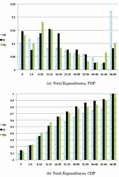
Figure 1 Data
Notes: Based on 1800 observations (600 per treatment).

Figure 2: The Amount of Internatlized Tax (0-16%)

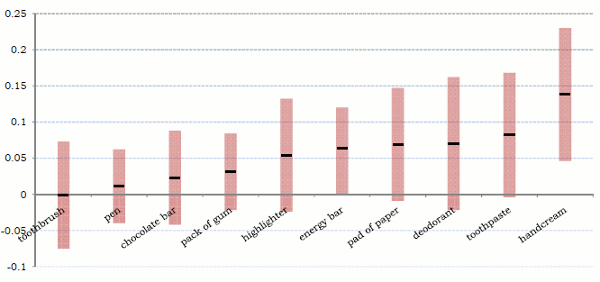
Figure 2 Data
Notes: The figure displays the amount (in percentage points) of the VAT that is internalized, on average, for each good. Zero reflects that the tax is completely ignored, whereas .16 represents all of the tax being internalized. The black horizontal bar displays the mean amount internalized, with the vertical bars indicating 95% confidence intervals.

Figure 3: Treatment Effect by Round (1-10)

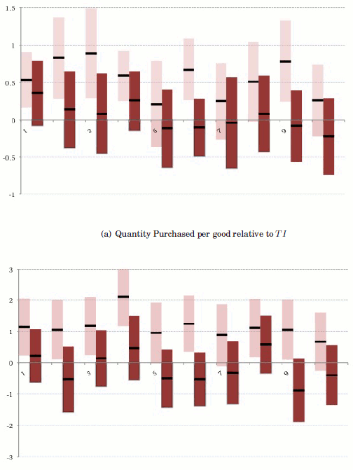
Figure 3 Data
Notes: Horizontal lines represent point estimates and vertical bars represent 90% confidence intervals. Light colored bars represent TE and darker colored bars represent TD.

Footnotes

* We thank Ziv Ben-Naim, Tomer Blumkin, Leif Danziger, Eyal Ert, Glenn Follette, Dan Silverman, Ro'i Zultan and seminar participants from Ben-Gurion University, the Federal Reserve Board, GMU, LMU, the 4th Psychology of Investment Conference, Office of Tax Analysis (US Department of Treasury), University of Michigan and UCSD for valuable comments. Ziv Ben-Naim provided excellent research assistance. We are grateful to Ben-Gurion University for funding the experiments. The analysis and conclusions set forth are those of the authors and do not indicate concurrence by the Board of Governors of the Federal Reserve Board or members of the research staff. All errors are our own. Return to Text

1. Our experiments were conducted in Israel where the VAT is 16%. Return to Text

2. It follows that industries can increase product demand by separating total prices into upfront fees and less visible taxes, service fees and other surcharges. With fees for checked baggage, meals, early boarding, flight changes, high fuel costs and, most recently, advance seat assignment, the airlines employ the widest and most creative range of price components. In fact, the Bureau of Transportation Statistics estimates that fees from checked baggage and reservation changes alone accounted for 4% of airline operating revenue and 62% of operating profit in the second quarter of 2011 (McCartney 2011). Other industries in which prices are commonly separated into components include banking, mutual funds and online retail. Return to Text

3. To be fair, the authors design a second test on alcohol pricing in which Hawthorne effects are not present. Return to Text

4. We will have more to say on this in Section 5. Return to Text

5. The marketing literature documents the effectiveness of "99" price endings in increasing demand (see, e.g., Anderson and Simester, 2003). Because only three of the 90 distinct prices in our experiments involve endings of 95 or more - slightly fewer than the number to be expected if price endings are drawn from a uniform distribution between 0 and 99 - and because altering one price necessitates two further price changes for the same good-discount rate combination in the other two treatments, we elected to leave all prices displayed as the straightforward multiplication of the retail price by the rate of discount. Return to Text

6. In a post-experiment questionnaire, we asked subjects what the VAT rate is. 76% of subjects answered correctly or within 1 percentage point. An error of up to one percentage point is understandable given that through five changes since 2004 the VAT rate in Israel has fluctuated between 15.5% and 17%. Return to Text

7. To be clear, the shopping-stage prices in have the 16% tax applied twice, one of which is refunded in the checkout stage. Thus, is the shopping-stage price and is the checkout price, as it is in the other two treatments. Return to Text

8. To illustrate this point, the Appendix contains screenshots of the shopping and checkout stages for a typical round of each of the treatments. Return to Text

9. The one exception is that a higher fraction of than subjects (5.2% versus 2.6%) spend nothing at the 80% discount rate. Return to Text

10. We do not employ logs in our main empirical estimation because of the large number of zeros (approximately 49% of observations) owing to the fact that subjects chose not to purchase about half of the five goods in a round on average. Thus, rather than make ad hoc adjustments to our dependent variable, we estimate our models in levels. Return to Text

11. As previously mentioned, this result is simply a multiple of the finding in column (3). For this reason and for brevity, we omit the analogous round-level results for quantity. Return to Text

12. To reconcile these opposing effects, subjects purchase relatively higher quantities of goods, but seem to switch to lower-priced goods at higher discount rates so that overall expenditures decline. Return to Text

13. Any other two rounds differ in the composition of goods and possibly also the discount rate. It is therefore easy to rationalize post hoc seeming preference reversals. Imagine, for instance, the following preferences: I prefer chocolate to toothbrushes if toothpaste is not offered, but I prefer a combination of toothbrushes and toothpaste over chocolate. Thus, if we were to compare consumption of chocolate to toothbrushes it may appear that there is a preference reversal when in fact this follows from the appearance of a new product (toothpaste). Return to Text

14. We do not count the purchase of one chocolate bar and one toothbrush in the second duplicate round as a violation of consistency because the subject continues to purchase (weakly) more chocolate than toothbrushes. Return to Text

15. These percentages can be understood as the theoretical probabilities of a preference reversal under the assumption of random choice conditional on sampling the random quantities without replacement from the subject's distribution of true quantities. For comparability with actual preference reversals, a preference reversal based on random choice is counted only in the case of a strict violation of transitivity. Return to Text

16. The other four items to be ranked for their naturalness are "you were offered to buy deodorant in an experiment," "the prices of these items were very different from the ones with which you are familiar," "you were asked to repeat the same purchasing task 10 times," and "you were paid on the basis of only one randomly chosen round." Return to Text

17. Recall that 49% of our quantity observations are zero. Rather than make ad hoc adjustments to this variable and given that we treat quantity as exogenous in this section, we simply restrict the estimation to positive quantities. Return to Text

18. Invoking the properties of log, recall that . Return to Text

19. The level of internalization is calculated as follows: 1.16 - exp( ). Return to Text

20. It is noteworthy that this result is nearly identical to that reported in Chetty et al. (2009). They find that individuals respond to a 10% increase in the tax as they would to a 3.5% increase in price. Return to Text

21. In a similar vein, based on an analysis of soft-drink sales, Colantuoni and Rojas (2012) conclude that consumers in Maine entirely ignored the introduction of a 5.5% soda tax. Return to Text

22. We use the more liberal 10% level of significance here for two reasons: (1) Tables 4 and 7 already have shown that the effect is slightly weaker in the second half of the rounds; (2) Table 7 showed that was not statistically significant. For both reasons, a 10% level allows us to detect individual rounds that may be marginally significant. Return to Text

23. Round 8 is significant at 11%. Recall that the goods offered were completely balanced across rounds. Hence, treatment differences over rounds cannot be the result of differences in the composition of goods by round across treatments. Return to Text

24. We did not allow and subjects to exceed 50 NIS during the shopping phase. Thus, faced with tax-inclusive prices, subjects never exceeded budget by design, while the shopping-stage limit implies that at checkout subjects could exceed their budget by no more than 8 NIS (equal to ). To enable subjects to spend the full 50 NIS after the VAT refund, they were permitted to exceed 50 NIS at the shopping stage. Return to Text

25. All rounds are included for subjects who never returned to their shopping cart. Return to Text

26. For the set of relatively inexpensive goods used in our experiment in which the highest tax-exclusive price is 8.86 NIS (deodorant at a discount rate of 50%), rounding up to the nearest shekel seems reasonable. For considerably more expensive goods, an alternative rule of thumb might be substituted whereby individuals round up to the nearest multiple of 100 NIS, for instance. Return to Text

27. Technically, for prices equal to six or more, we add one shekel and then round up or down to the nearest half shekel. This is because 16% of six is roughly equal to one and thus becomes a very simple rounding heuristic to apply. Return to Text

28. We acknowledge the existence of many alternative ways to round prices in addition to the two simple and plausible ones that we consider. For example, subjects may round on or on particular bundles of related goods. The choice of more complicated and less intuitive rounding rules would be ad hoc and any attempt to define precise rounding rules for the entire set of these more complicated situations would quickly become unwieldy. We therefore content ourselves with these two rounding heuristics, leaving it to others to explore other rounding mechanisms. Return to Text

29. We assume here standard upward sloping supply and downward sloping demand curves. Return to Text

30. Even if we assume that producers cannot adjust prices to incorporate the sales tax in the short run, the increased government revenues can be partially used to compensate producers such that they are no worse off. Return to Text

^♣ This version is optimized for use by screen readers. Descriptions for all mathematical expressions are provided in LaTex format. A printable pdf version is available. Return to Text

Home | Economic Research and Data | Accessibility | Contact us
Last update: February 14, 2013