
The Dynamics of Labor Maret Polarization
AbstractIt has been well documented that the share of the working-age population employed in "middle-skill" occupations has been falling for some time, while the share in lower- and higher-skill jobs has been rising--i.e. "polarization" of the labor market (e.g. Autor 2010). However, the dynamics and related mechanism behind these employment trends are not fully understood; nor is it well understood what happens to workers who are displaced from middle-skill jobs. In this paper, I use data from the matched monthly CPS, the March CPS supplement, and the Displaced Worker Survey to answer two primary questions. First, into what employment states or occupations do unemployed persons who were formerly employed in low-, middle-, or high-skill occupations transition? Second, how have transitions between job types and employment states changed over time, and how have these changes contributed to trends in employment shares by job-type? I find that the decline in the share of workers in middle-skill jobs is due both to a decline in inflows into these jobs (particularly from non-employment and for younger workers) and because of a rise in outflows from these jobs (to non-employment and to other jobs); the increase in the share of workers in lower-skill jobs appears due to an increase in worker transitions from other job types (evident within all demographic groups); and the increase in the share of workers in higher-skill jobs appears due to an increase in worker transitions from other job types and is also somewhat compositional in nature (because there are more college-educated workers).
Disclaimer: Any opinions and conclusions expressed herein are those of the author and do not indicate concurrence with other members of the research staff of the Federal Reserve or the Board of Governors.
Acknowledgements: Many thanks to Christopher Nekarda for providing matched monthly CPS data, and David Lebow for helpful comments. Thanks to Devin Saiki and Erik Larsson for research assistance. All errors are my own.
I.Introduction
It has been well-documented that the U.S. labor market has become more polarized over the last few decades--that is, employment growth has been more concentrated in the highest and lowest paying occupations (e.g. Autor 2010). Some of the earliest research centered on establishing a theoretical framework for understanding the nature and implications of recent technological change (Autor, Levy, Murnane 2003), and applying this framework to a model of relative labor demand for different skill-types (Autor, Katz, and Kearny 2006). Subsequently, researchers have demonstrated the pervasiveness of polarization across developed countries (Manning, Goos, and Salomons 2009 and 2011; Michaels, Natraj, and Van Reenen 2013),1 and focused greater attention towards testing competing hypotheses for polarization (i.e. openness to global markets versus technological change, e.g. Autor, Dorn and Hanson 2013a and 2013b).
Other recent research has questioned whether polarization in labor demand is at least in part responsible for the weakness of the last three labor market recoveries. For example, Jaimovich and Sui (2012) point out that labor market polarization accelerated following the 1990 and 2000s recessions. They hypothesize that this may be because displacement of workers from routine occupations (generally, "middle-skill" or middle-paying jobs) was concentrated around those recessions, and these types of workers may take time to transition into other types of jobs (or remain permanently out of the labor force). Nevertheless, others have argued that accelerated labor market polarization does not appear responsible for the most recent labor market downturn or subsequent slow recovery, in part because unemployment rates and job finding rates have evolved similarly for workers regardless of what type of job they were displaced from (Foote and Ryan 2012; Albanesi et. al. 2013; Tuzemen and Willis 2013).
Despite a burgeoning literature related to labor market polarization2, there are still many unanswered questions related to the potential implications of polarization. For example: How have these changes affected younger persons' education or career choices? Is polarization an important explanation for the decades-long decline in labor force participation for prime-age men (particularly men without a college degree)? What happens to "middle-skill" workers who are displaced from their jobs--do they remain in the middle-skill labor market, or do they somehow transition to the higher- or lower-skill labor markets? And, more ambitiously, how do these structural changes affect the cyclical dynamics of the labor market and longer-run growth prospects of the U.S. economy (is labor market polarization responsible for jobless recoveries)?
This paper attempts to make progress on some of these issues by using a variety of data sources to explore the following specific questions:
- What happens to middle-skill workers when they become unemployed?
- How have transition rates between employment states and job types changed for low-, middle-, and high-skilled jobs, and how have these changes contributed to observed labor market polarization (i.e. to changes in the aggregate share of workers employed in these jobs)?
Thus, the purpose of this paper is to explore the dynamics that underlie changes in employment shares by job type, by examining the transition rates into and out of job types. In doing so, this research helps "explain" why the share of workers in middle-type jobs has been falling over time, and contributes towards understanding the mechanisms behind polarization. For example, one intuitive and plausible theory for why the share in middle-type jobs is falling is that, as technological change and globalization have reduced demand labor in for middle-type jobs, these workers are involuntarily displaced. Because these workers tend to be less-educated, and because labor demand seems to be increasingly biased towards college-educated labor, one might expect that displaced middle-type workers either retrain and attain a high-type job, or perhaps more likely, accept the new realities of the labor market and drop into the lower-type, service sector labor market (or drop out of the labor market entirely). This is an intuitively appealing theory, and it often appears often in the press when describing the "plight of the middle-class." It also forms the basis of some recent hypotheses about jobless recoveries (Jaimovich and Siu 2012), and may have implications for the speed of future labor market improvement. An alternative theory--with potentially less harmful consequences--is that the share of workers in middle-type jobs is falling because hiring rates into these sorts of jobs have declined and employment shares have fallen due to attrition (consistent with the observation in Autor and Dorn 2009 that the average age of middle-type jobs has risen). For instance, fewer young workers could be entering the middle-skill labor market, perhaps because they are going to college in greater numbers and subsequently entering the high-skill labor market. Of course, these explanations are not mutually exclusive, but they do have different policy implications.3 Examining trends in transition rates from unemployment to employment by job-type, conditional on the worker's former job-type, as well as longer-run transition rates from one job-type to another, can help differentiate these hypotheses.
In this paper, I proceed by first discussing my choice of occupational categorization by job type. I then show trends in polarization, demonstrate that polarization is even more apparent within age/education group (and hence masked in the aggregate due to compositional demographic changes), and show that polarization has been concentrated around recent recessions (as shown in Jaimovich and Sui 2012). Next, I use a multitude of data sources to examine trends in what happens to unemployed workers by job-type (i.e. with what frequency do they transition to non-employment or jobs of other types), and then I examine trends in transition rates unconditional on employment status (i.e. with what frequency do employed workers switch job types, and how has this changed over time).4 Finally, I assess the degree to which changes in inflow and outflow rates by job type have affected aggregate employment shares. I do this by examining the evolution of counterfactual shares that hold inflow or outflow rates fixed at some earlier level.
One key finding of this paper is that the share of workers in middle-skill occupations has been declining over the past few decades in part both because the outflow rate from these jobs (to non-employment as well as to jobs of other types) has been increasing and because the inflow rate to middle-skill jobs from non-employment or jobs other types has also been declining (particularly for younger workers).5 Thus, the labor market dynamics of polarization are complicated, depending on changes in the rate of inflows and outflows by job-types, and differ across demographic groups. Any theories regarding the labor market impact of polarization (e.g. on the weakness of the aggregate labor market since the 1990s) should therefore recognize the importance of trends in both inflows and outflows rates by job types.
II. Defining labor market polarization, and trends in employment by job type
1.Defining type of job by occupation
"Labor market polarization" has been defined in a variety of manners. From its most theoretical founding, "polarization" has been used to refer to differences in employment and wage growth between routine occupations (i.e. jobs that primarily require tasks that can be codified and follow explicit rules and instructions) and non-routine occupations.6 Common examples of routine occupations include bank tellers, non-supervisory production workers, and administrative assistants. Non-routine occupations are often divided into manual jobs (e.g. service sector jobs: retail clerk, food service, child care, landscaping, etc.) and cognitive jobs (e.g. professional, managerial, and technical jobs).
This division (routine, non-routine cognitive, and non-routine manual) is often chosen because it naturally maps into theories of the impact of technological change and/or globalization on labor demand. For instance, as computing power and automation technology becomes cheaper, and as it becomes easier to physically separate the act of production from product design, marketing, etc., then demand for routine occupations in the U.S. should fall, demand for non-routine cognitive occupations should rise (because workers in these occupations are made more productive by the cheaper technology and openness to new labor/product markets), and relative employment and wages for non-routine cognitive jobs should increase. Non-routine manual jobs, which are performed locally and are harder (as of yet) to substitute with machines or foreign labor, are not directly affected by these changes.7 Categorizing occupations in this manner also makes explicit that polarization is a cross-industry phenomenon, rather than simply an outcome of sectoral shifts (e.g. Foote and Ryan 2012, and Tuzeman and Willis 2013)--that is, polarization is not simply the outcome the long-run downtrend in manufacturing employment, but is also evident within industries.8
There are also other categorizations of occupations that yield similar insights. For instance, it is also common in the literature to divide jobs into high-, middle-, and low-skill (Autor 2010, Abel and Deitz 2012, Foote and Ryan 2012) where "high-skill" refers to CPS-defined occupational categories "managers, professionals, and technicians", middle-skill refers to "office administration, production craft and repair, and operators, fabricators and laborers", and low-skill refers to "food-preparation, building and grounds cleaning, personal care and personal services."9 And another common division is into high-, middle-, and low-wage jobs (Autor, Katz, and Kearney 2006; NELP 2012).
In this paper, I divide jobs, based on occupation, into four "types":
- High-type: Managerial/supervisory, professional, technician
- Middle-type: Non-supervisory office administration and goods production
- Low-type: Non-supervisory personal service, food preparation, and sales
- Other: Non-supervisory construction, extraction, transportation, or other
Table 1 provides some summary statistics for these four job types. The first type has higher wages, on average, than the rest, and over half of those employed in this type have a bachelor's degree or better. The second type has lower wages than the first type, but higher than the third type; all types other than the first type tend to be non-college educated, though the second type is more likely to have a high school degree than the third type.10 The final job category includes construction, extraction, repair, transportation, and laboring jobs. Workers in these jobs tend to be better paid than the middle- or low-type jobs, but also are less likely to have a high school degree. The primary reason I separate these jobs from other lower-type jobs is that they are predominantly male, are concentrated in construction-related jobs, tend to be more cyclical, and--as I discuss later (and show in Figures 1A and 1B)--employed a roughly constant share of employment over the previous decades (the most pronounced movements in employment shares are in the other job types).11 Since the first three job types align (roughly) monotonically by wage and education, in this paper I refer to them as high-, middle-, and low-type jobs (explicitly avoiding "skill-type" or wage). Also note that this taxonomy maps nicely into the routine/non-routine categorization laid out by theory: high-type tend to specialize in non-routine cognitive tasks (nearly all are in the top half of jobs when arranged by how intensively they use non-routine cognitive tasks, as defined as in Autor, Levy and Murnane 2003); middle-type tend to specialize in routine tasks (nearly all are in top half of jobs, when jobs are arranged by use of routine tasks); and low-type jobs (and "other" jobs) tend to specialize in non-routine manual tasks. For these reasons, and also because this categorization is well-defined by easily understood occupations, for the rest of the paper I follow this high-, middle-, and low-type taxonomy. Table 1 also shows the share of each job that is from a particular age/gender group, and the share of each age/gender group (conditional on employment) in each of the four job types. Unsurprisingly, younger workers tend to be in low-type jobs, non-college workers are rarely observed in high-type jobs, and women are rarely observed in the other-type jobs.
2. Accounting for breaks in occupational coding
One difficulty in classifying jobs into type based on occupation is that the coding of occupations in the CPS changes over time. The focus of my analysis is from 1983 to the present12, and this period includes three instances when some occupations are re-classified: between 1991 and 1992, between 2002 and 2003, and between 2010 and 2011. Of these three reclassifications, the 1991/1992 is the most innocuous and only involved reclassification of a handful of occupations. For these, I matched occupations in 1992 to occupations in 1991 discretionarily (by hand). The reclassification between 2002 and 2003 was significantly more extensive. Rather than matching by hand, I exploited the fact that some CPS respondents can be matched from one month to the next. I kept individuals observed to be employed in the same occupation in November and December 2002 (under the 2002 coding scheme), observed to be employed in the same occupation in January and February 2003 (under the 2003 coding scheme) and reported having stayed at the same job between December and January. I then created the full universe of occupational correspondences between the 2002 and 2003 schemes, and created a probability-weighted crosswalk between the two.13 Because one-to-one correspondences appear very rarely between the 2002 and 2003 occupation coding schemes, for observations in 2003 and later, I assign each employed individual a probability of being in a particular 1990s-coded occupation based on this weighted matrix of 2002/2003 occupation matches. (I use a similar procedure for the 2010/2011 change in occupational coding, although the differences in the occupational classifications are modest compared to the 2002/2003 switch.) The upside to this procedure is that there appears to be no trend break in employment by job-type between the seam breaks in occupational coding, as has appeared in other work that examines trends in employment by occupation-type over time. The downside is that the reassignment of occupation is dependent on only four months of data (two months on either side of the seam break).14 It is also worth noting that proper accounting for the change in occupational coding is extremely important for analysis about cyclical dynamics of polarization, since the 1991/1992 and 2002/2003 changes occurred in the midst of the "jobless recoveries."
3. Trends in polarization
Figure 1A shows the 12 month moving average of the share of the 16+ population in each of the four job types defined above, as well as the share not employed (the estimates are constructed using monthly CPS data).15 The share of adults in high-type jobs (blue line) rose by about 5 percentage points since 1985, the share in middle-type jobs (maroon line) fell by about 5 percentage points, the share in low-type was roughly flat, and the share in other trended down modestly. Conditional on being employed (Figure 1B), the decline in the share employed in middle-type jobs is larger (falling from 25 percent of the employed population in 1985 to just above 15 percent in 2012). In the aggregate the clearest shift in employment by occupation appears to be from the middle-type jobs to high-type.
However, these aggregate trends mask important within-group changes. Figures 2A, 2B, and 2C plot the share of each of six demographic groups employed by job-type (conditional on being employed). Figure 2A shows that, within demographic groups, the share employed in high-type jobs has substantially increased only for older workers--hence, much of the aggregate rise shown in Figures 1A and 1B is because an increasing share of the population is college-educated, and college-educated workers tend to be in high-type jobs. Figures 2B and 2C are illuminating: for younger workers and those without a college degree, the share in low-type jobs has risen by roughly as much as the share in middle-type jobs has fallen. For college-educated, prime-age men and women, the share in low-type jobs has increased modestly since the early 2000s as the share in middle-type jobs has fallen (for females, these trends also correspond with a rise in the share employed in high-type occupations).
To summarize: over this entire period, the share in middle-type jobs has fallen for all types of workers. The declines have been most significant for younger workers and non-college workers, and for these groups the decline in middle-type employment has been almost entirely mirrored by an increase in low-type employment. And even for college-educated workers, there is a modest increase in the share employed in low-type jobs since the early 2000s.16
4.Labor market polarization around recent recessions
Jaimovich and Siu (2012) note that polarization appears to have been most pronounced around the recent jobless recoveries. Relatedly, Smith (2011) noted that the share of adults in jobs that teens tend to do (i.e. low-type jobs) discretely jumped up around the jobless recoveries, corresponding with discrete drops in youth employment and participation rates. Figures 3A, 3B, and 3C also show this, using the high-, middle-, low-type classification previously described. These Figures show the three-month moving average of employment in a given job-type (constructed using monthly CPS microdata), normalized to 100 at the peak of aggregate CPS employment (March 1990, March 2001, and December 2007 respectively). Because analysis of the dynamics surrounding these episodes is not entirely robust to one's choice of de-trending or filtering, I present simple three month moving averages. Construction and extraction occupations are highly cyclical--hence the annual swings. However, despite some cyclicality in employment in the other occupations, it is quite clear that following the 1990 and 2001 recessions, employment in middle-type occupations failed to recover to pre-recession levels, while employment in other industries eventually did. Jaimovich and Siu (2012) show that, if following these recessions employment in middle-type occupations evolved as it historically did, then aggregate employment would have recovered much sooner and the recoveries would have been significantly less "jobless." Figure 3C clearly shows that employment growth fell significantly and remained weak for all types of jobs following the most recent recession, although it does seem that employment in high- and low-type jobs has recently improved somewhat faster than employment in middle-type jobs.
Table 2 displays percent changes in the twelve-month moving average of employment (and share employed, conditional on being employed) by job type and demographic group.17 One important observation is that, within an age or education/gender group, the increase in the share employed in low-type jobs (conditional on employment) is generally larger than the overall share employed in these low-type jobs; this is because the college-educated share is growing, and these workers are less likely to work in low-type jobs. Also of interest is that following each recession, the share of younger and non-college persons in middle-type jobs typically fell by more (and the share in low-type jobs typically rose by more) than the aggregate share.
III. Inflows and outflows by job-type
1.Transition rates from unemployment
In this section, I present a variety of evidence regarding transition rates from unemployment to employment, by type of former job and current job. The primary focus is to uncover what happens to persons unemployed from middle-type jobs, though the experience of unemployed persons who had previously worked in other types of jobs is also of interest.
i. Monthly transition rates (matched CPS data)
To begin, I use matched monthly CPS data18 to examine the probability that a person unemployed in month t-1 (who had been displaced or quit from a previous job, and reported the occupation of his or her previous job) is observed in a job of a particular type (or non-employed) in month t. These monthly transition probabilities are displayed in Figure 4. The top three panels show the probability that an unemployed worker in month t-1 who was formerly employed in a job type other than j, was observed to be employed in job type j in month t. (For visual ease, the plots do not show the probability that an unemployed worker from type j was observed as employed in type j.) For example, the plot in the middle of the top panel shows the probability that an unemployed worker in t-1 who was previously employed in a high-type (blue line), low-type (green line) or other-type (orange line) job was observed as employed in a middle-type job in t. That is, the top row shows the inflow rate to various job types from unemployment, where each panel focuses on inflows to a particular job type. The bottom row shows similar transition rates, except each panel focuses on transitions from being unemployed of a particular job type. For example, the plot in the middle of the bottom panel shows the probability that an unemployed worker in t-1 who was previously employed in a middle-type job was observed employed in a high-type (blue line), low-type (green line), or other-type (orange line) job in t (or observed as non-employed, the black line).19
A few observations related to transitions to and from middle-type jobs:
- There is a steady decline in the rate at which unemployed workers from non-middle-type jobs transition to middle-type jobs (top middle plot)--that is, the inflow rate to middle-type jobs from unemployed formerly non-middle-type workers appears to be falling over time. Further, these transition rates appear to drop discretely following the 1990, 2001, and most recent recessions.
- There is no evidence of an increase in the rate at which unemployed middle-type workers transition to non-middle-type jobs (bottom middle plot). Instead, there is an upward trend in the rate at which these workers remain non-employed, though this is true of unemployed workers of all types.
ii. Monthly transition rates (matched CPS data), by duration of unemployment
Figure 4 shows that, at least on a month-to-month basis, there is no evidence that former middle-type workers are transitioning to low- or high-type jobs at an increasing rate. But perhaps such transitions are more likely for those who are unemployed for longer, because these persons may have given up on the on the possibility of transitioning back to a middle-type job. To explore this possibility, in Figure 5 I estimate similar transition rates (for formerly middle-type workers, and into middle-type jobs), conditional on whether the respondent in t-1 was unemployed for a short duration (1-13 weeks), middle duration (14-26 weeks) or long duration (27+ weeks). Although these data are significantly noisier, there is no evidence that former middle-type workers have become increasingly willing to transition to low-type jobs, or that the propensity to transition to low-type jobs is higher for those unemployed longer. In fact, the reverse is true--those who are unemployed for a shorter length of time are more likely to transition to a low-type job, and those who are unemployed longer are more likely to remain in non-employment. Also of note is that the decline in the likelihood that non-middle-type unemployed workers transition to middle-type jobs is apparent only for the short-term unemployed (upper-left panel).
iii.1, 4, 8, and 12 month transition rates (matched CPS data)
It is also possible to track individuals who remain in the CPS sample over four month, eight month, and twelve month periods. Perhaps it is the case that, although unemployed middle-type workers are not increasingly likely to transition to non-middle-type jobs on a month-to-month basis, they are willing to do so over longer horizons. The top panels of Figure 6 plot the probability that a former non-middle-type worker observed to be unemployed in month t-1, t-4, t-8, or t-12 is observed employed in a middle-type job in month t. The bottom panel plots the probability that an unemployed former middle-type worker transitions to a non-middle-type job over the same horizon as the top panel. As with the one-month transition plots (i.e. Figure 4, or the left-most panels in Figure 6), there is a long-run decline in the likelihood that someone unemployed from a non-middle-type job has transitioned to a middle-type job when observed 4, 8, or 12 months later (the top panel), although--in contrast with the one-month transitions--there is some evidence that unemployed middle-type workers may be increasingly likely to transition to high-type jobs over time (the blue line in the right three plots in the bottom panel, i.e. when observed 4, 8, or 12 months later).20
iv. Transition rates from the Displaced Worker Survey
Every two years, the BLS includes a supplement to the CPS survey (usually in January or February) that asks specific questions to the subsample of respondents who report being involuntarily displaced from employment at some point over the preceding few years (three to five years, depending on the year of the survey). For persons who report having been displaced, the Displaced Worker Survey (DWS) then asks questions about the previous job (length of tenure, previous wage, and occupation/industry). Hence, because the DWS provides information about a respondent's current and previous occupation, the DWS is an additional source of information about transition rates from one type of job to another.
Similar to Figure 4, Figure 7 shows the probability that someone displaced from a job of a particular type at some point in the previous three years is observed employed (or non-employed) at the time of the survey. For instance, the middle plot of the top panel shows the probability that a person displaced from a high-, low-, or other-type job at some point in the previous three years was observed as employed in a middle-type job in year t. Conversely, the middle plot of the bottom panel shows the probability that a person displaced from a middle-type job was observed as employed in a non-middle-type job in year t.
Given that the sample sizes are smaller than the usual CPS survey, the data are quite noisy. Nevertheless, there is some evidence that workers displaced from high- or low-type jobs are less likely to be re-employed in middle-type jobs (top middle plot), and some hint that workers displaced from middle-type jobs are somewhat more likely to be employed in high-type jobs, at least relative to the late 1980s (the blue line in the bottom middle plot).
v. Summary
To summarize the findings thus far, the variety of data on transition rates from unemployment to employment provide little to suggest that unemployed middle-type workers are increasingly likely to transition to a non-middle-type job; instead, they are increasingly likely to remain non-employed, though this is also true for unemployed workers who were employed in other types of jobs as well. The most striking and consistent trend is that unemployed non-middle-type workers are increasingly less likely to transition to middle-type jobs than in the 1980s. That is, inflow rates to middle-type jobs from non-middle-type unemployment have fallen, and seem likely to contribute, at least in part, to the declining share of employment in these jobs.
2. Transition rates, unconditional on employment status
The flows in the previous section represented transitions from unemployment to employment. However, changes in aggregate employment shares are also affected by the rate at which employed workers switch job types. One way that this could matter is if, for instance, younger non-college workers tended to start in low-type (service sector) jobs before transitioning into more permanent employment in middle-type jobs (e.g. manufacturing). This section uses matched CPS data (at 1, 4, 8, and 12 month spans), and data from the March CPS supplement to examine job-to-job transition rates, by job type, for respondents employed in previous months.21
i. 1, 4, 8, and 12 month transition rates (matched CPS data)
Figure 8 uses matched monthly CPS data to calculate one-month transition probabilities unconditional on employment status in month t-1. In any given month, the probability that an employed person changes to a different type of job is fairly small (no higher than 5 percent--the sum of the colored lines in any of the plots). Of note, there is a modest increase in the likelihood that someone employed in a middle-type job in month t-1 transitions to a high- or low-type job in month t (the maroon lines in the upper right and upper left panels). Also, the probability of transitioning from non-employment to a middle-type job (the black line in the middle-top plot) has been falling over time, and the decline accelerated following the 2001 and most recent recession.
Over longer periods of time, the probability that an employed person is observed to transition to a different type of job should be higher. As in the previous section, I exploit the fact that matched CPS data allows one to examine transitions at longer horizons (up to 12 months). Figures 9A, 9B, and 9C plot the probability that someone observed in a particular job type (or non-employed) 1, 4, 8, or 12 months previously, is observed in month t to be employed in a particular job type. Figure A plots transitions into and out of high-type jobs, and Figures B and C plot similar transitions for middle- and low-type jobs, respectively.22
Some observations of note:
- For all horizons, the rate at which persons from low- or middle-type jobs transition to high-type jobs is rising over time (the top panel of Figure 9A). This is particularly true for the transition rates from middle-type jobs.
- Conversely, the rate at which persons transition from low-type jobs to middle-type jobs is falling over time, particularly over longer transition horizons (8 months or 12 months--the top right panels of Figure 9B).
- Further, the rate at which the non-employed transition to middle-type jobs is also falling modestly over time (top right panels of Figure 9B).
- There is essentially no trend in transitions out of high-type jobs, and there is, if anything, only a modest trend in the transition rate out of low-type jobs (bottom panel of Figures 9A and 9C). In striking contrast, the rate at which persons employed in middle-type jobs transition to high- or low-type jobs, or non-employment, is increasing over time, and the upward trend is steeper for longer transition horizons (bottom panel of Figure 9B).
ii. Annual transition rates (March CPS)
I use the March supplement to the CPS as another way of looking at unconditional annual transition rates. The March supplement provides information on respondents' employment status and primary occupation in the previous year, and combining this with information on respondents' current employment status and occupation, I construct the rate at which persons who report being employed in the previous year (and who report a primary occupation in the previous year) transition to different job types as observed in March. These transitions are reported in Figure 10. For example, I estimate the probability that a person who was primarily employed in a middle-type job in the previous year is observed to be employed in a non-middle-type job in March (the middle plot in the bottom panel of Figure 10).
Although these data appear noisy, there are a few observations of note:
- The rate at which non-middle-type workers transition to middle-type jobs has been falling over time--particularly for low-type and other-type workers--and the trend appears to accelerate around recessions (the green and orange line in the middle of the top panel).
- The rate at which middle-type workers transition to non-middle-type jobs has, if anything, fallen over time (the blue, green, and orange lines in the middle of the bottom panel).
iii.Summary
Putting this all together, evidence from matched CPS data and the March Supplement suggests that since at least 1995 the probability that someone who is in a non-middle-type job or non-employed will transition to a middle-type job over the next year (the inflow rate to middle-type jobs from non-middle-type jobs) has fallen. It also seems (from the longer-horizon matched CPS data) that middle-type workers are more likely to transition to a low- or high-type job over the next year (the outflow rate from middle-type jobs has also risen). These findings, combined with the evidence in the previous section that persons unemployed from non-middle-type jobs are less likely to find middle-type employment, suggests that both trends in inflow and outflow rates contribute to the declining share of workers in middle-type jobs. In the next section, I analyze more quantitatively the contribution of trends in these inflow and outflow rates to changes in employment shares by job type (i.e. labor market polarization).
IV. The contribution of trends in inflow and outflow rates by job-type to trends in employment shares and polarization
1. Defining the four transition rates into and out of job types
The previous analyses suggested that the share of workers in middle-type jobs has declined because fewer non-middle-type workers (or unemployed, formerly non-middle-type workers) are transitioning to middle-type jobs, and also because middle-type workers (or unemployed, formerly middle-type workers) are less likely to remain in middle-type jobs. In this section, I attempt to quantify the importance of changes in inflow and outflow rates, and also examine whether these changes are more significant for some demographic groups than for others.
To begin, I define four flows that may affect the stock (or share) of persons in a particular job type: the inflow rate from non-employment, the inflow rate from employment of another type, the outflow rate to non-employment, and the outflow rate to employment of another type. In the top panel of Figure 11, I provide a plot that gives the flavor of what such one-month and twelve-month transition rates look like for middle-type jobs. Confirming the previous analyses, one-month transition rates from non-employment to middle-type jobs have fallen (the green line in the upper-left), and the rate at which middle-type workers transition (at a one-month or twelve-month horizon) to other types of employment has increased substantially (the red line). The top four rows of panels A and B in table 3 provide estimates of changes in these transition rates for all four job types (the changes are estimated between 1997-1999 and 2009-2011). Notably, for both transition horizons, the inflow rate to high- and low-type jobs from other jobs has risen, and the outflow rate from middle-type jobs to non-employment and other types of jobs has also risen.
2. How inflow and outflow rates relate to employment shares
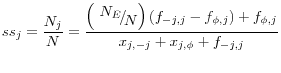
How do changes in these inflow and outflow rates affect the actual stock and share of employment by job-type? To answer this question, I begin by constructing steady-state employment shares as a function of these 16 inflow and outflow rates (four inflow/outflow rates for four job types). I then construct counterfactual employment shares by fixing inflow or outflow rates at some earlier value, and examine how these counterfactual shares would have evolved had this particular flow not changed. The difference between one of these counterfactual shares and the actual share suggests how much of the change in the actual share might be accounted for by changes in the inflow or outflow rate. For instance, holding the inflow rate to middle-type jobs from non-employment fixed at an earlier level, estimating the implied counterfactual share employed in middle-type jobs, and comparing the change in that counterfactual share to the actual share provides some indication regarding whether changes to this inflow rate is an important contribution to the decline in the share of workers in middle-type jobs.
To be more concrete, assuming that the number of workers in a job of type j is in steady state, then the number of workers in month t entering job j should equal the number of workers leaving job j (where
![]() is the number of persons not in job j in the previous month,
is the number of persons not in job j in the previous month, ![]() is the rate at which persons not in job j find employment in job j between months t-1 and t,
is the rate at which persons not in job j find employment in job j between months t-1 and t, ![]() is the number of workers in job j in t-1, and
is the number of workers in job j in t-1, and ![]() is the rate at which persons in
job j exit employment between months t-1 and t: 1)
is the rate at which persons in
job j exit employment between months t-1 and t: 1)
![]()
Rearranging, defining N without a subscript as the working-age population, and dropping the time subscript (assuming a steady-state), the steady-state share of the working-age population employed in job type j (unconditional on employment) is:232)
![]()
Next, to incorporate the four inflow/outflow rates described in the previous subsection, define:
 as the rate at which workers not in job j transition to job j (the inflow rate from non-j employment)
-
 as the rate at which non-employed persons transition to job j (the inflow rate from non-employment)
  as the rate at which persons employed in job j transition to a non-j job (the outflow rate to non-j employment)
-
 as the rate at which persons employed in job j transition to non-employment (the outflow rate to non-employment)
Using these four flows (and defining
![]() as the number of non-employed persons and
as the number of non-employed persons and ![]() as the number of
employed persons), one can define the steady state relationship, for which the number of inflows into a job type equals the outflows, as: 3)
as the number of
employed persons), one can define the steady state relationship, for which the number of inflows into a job type equals the outflows, as: 3)
![]()
Rearranging: 4)
And the steady-state share employed in job j, conditional on being employed, is: 5)
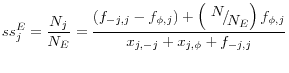
This expression includes
![]() , which itself is a function of the 16 flows. To get rid of this expression in the equation for the steady-state shares, note that the four shares
, which itself is a function of the 16 flows. To get rid of this expression in the equation for the steady-state shares, note that the four shares ![]() add up to 1. Using this equality, and rearranging, we can define (where j is 1, 2, 3 or 4):
add up to 1. Using this equality, and rearranging, we can define (where j is 1, 2, 3 or 4):
6)
![\displaystyle \frac{N}{N_{E} } =\frac{\prod _{i=j\{ 1,2,3,4\} }\left(x_{i,-i} +x_{i,\phi } +f_{-i,i} \right) -\sum _{i=j\{ 1,2,3,4\} }\left[(f_{i,-i} -f_{\phi ,i} )\prod _{k=-i}(x_{k,-k} +x_{k,\phi } +f_{-k,k} ) \right] }{\sum _{i=j\{ 1,2,3,4\} }\left[f_{\phi ,i} \prod _{k=-i}(x_{k,-k} +x_{k,\phi } +f_{-k,k} ) \right] }](img20.gif) Plugging (6) in to (5), we can define any steady state as a function of all 16 flows. These steady states will evolve over time as the inflow and outflow rates change--though with no change in the flows, the conditional employment shares would settle down to these rates (again, analogous to
a steady-state unemployment rate, e.g. Shimer 2012, Barnichon and Nekarda 2012). With these objects we can then estimate what would have happened to the conditional steady state share if any of the four flows remain fixed at some previous rate. For instance, suppose we hold the rate at which
non-employed persons flow into middle-type jobs fixed at some earlier (average 1997-1999) level, and define the resulting steady state share employed in middle-type jobs as
Plugging (6) in to (5), we can define any steady state as a function of all 16 flows. These steady states will evolve over time as the inflow and outflow rates change--though with no change in the flows, the conditional employment shares would settle down to these rates (again, analogous to
a steady-state unemployment rate, e.g. Shimer 2012, Barnichon and Nekarda 2012). With these objects we can then estimate what would have happened to the conditional steady state share if any of the four flows remain fixed at some previous rate. For instance, suppose we hold the rate at which
non-employed persons flow into middle-type jobs fixed at some earlier (average 1997-1999) level, and define the resulting steady state share employed in middle-type jobs as
![]() =
=
![]() . The change in this object is the change that would have occurred in the (steady-state) share employed in middle-type had the
inflow rate from non-employment not fallen over this period. Hence, the difference between the change in the actual share employed in middle-type jobs and this counterfactual change gives a sense of the contribution of changes in the inflow rate from non-employment. That is, if
. The change in this object is the change that would have occurred in the (steady-state) share employed in middle-type had the
inflow rate from non-employment not fallen over this period. Hence, the difference between the change in the actual share employed in middle-type jobs and this counterfactual change gives a sense of the contribution of changes in the inflow rate from non-employment. That is, if
![]() (the change in the actual share) is similar in magnitude to
(the change in the actual share) is similar in magnitude to
![]() the change in the steady state counterfactual share) then the change in the inflow rate from non-employment was not important for
explaining the change in the actual change. If instead, the change in the counterfactual steady-state share is much different from the actual change, then the change in this flow was important.
the change in the steady state counterfactual share) then the change in the inflow rate from non-employment was not important for
explaining the change in the actual change. If instead, the change in the counterfactual steady-state share is much different from the actual change, then the change in this flow was important.
3. The importance of inflow and outflow rates to polarization over the last decade
To begin, I use these steady-state employment shares and counterfactual employment shares to examine the contribution of trends in inflows and outflows to polarization since the late-1990s.24 The bottom panel of Figure 11 gives a flavor of what this analysis looks like. In the bottom left, one-month transition rates to and from middle-type jobs are held at their 1997-1999 levels; in the bottom right, twelve-month transition rates are held fixed. Both pictures suggest that, had the flow of middle-type workers into non-middle-type jobs not risen over this period, then the share of workers in middle-type jobs would have been significantly higher. The counterfactual analysis using one-month transition rates suggests that the declining inflow from non-employment was equally important towards explaining the decline in middle-type employment over this period.
The bottom rows of panels A and B in table 3 provide estimates of the steady state share consistent with the estimated one-month transition rates (panel A) or twelve-month transition rates (panel B). A few observations of note:
- Regardless of the transition horizon considered, the share of employment in high-type jobs would not have increased nearly as much if not for the increase in the inflow rate from other jobs. For instance, the share in high-type employment increased by 4 percentage points over this period. Had the inflow rate from other jobs not risen, the share in high-type employment would have increased from between 0.4 percent (holding the twelve-month transition rate fixed) to 1.3 percent (holding the one-month transition rate fixed).
- One reason why the share employed in middle-type jobs has fallen is because the outflow rate to other job types has risen substantially (at both the one- and twelve-month transition horizon). Also, from panel A, the share in middle-type jobs would not have fallen nearly as much as it did if the inflow rate from non-employment had not fallen, though the decline in this inflow rate is somewhat less important at the twelve-month horizon.
- The primary reason why the share of workers in low-type jobs has increased is because the inflow rate from other employment (at both the one- and twelve-month horizons) has increased significantly.
4. The importance of inflow and outflow rates to polarization since the mid-1980s, and differences by demographic groups
i. Changes in inflow and outflow rates, and counterfactual employment shares
As mentioned previously, month-to-month transition rates cannot accurately be compared for years pre- and post-CPS redesign. However, twelve-month transition rates are more likely to be comparable.25 In table 4, I provide results from a similar counterfactual exercise estimated over a longer period (1987-89 to 2009-11). The first three rows of each panel show estimates of changes in unconditional and conditional employment shares, and conditional shares estimated "in-sample" (i.e. for all observations that can be matched for calculating twelve-month transitions.) The next four rows show the change in average twelve-month inflow and outflow rates. The final rows show the steady state conditional employment share, and the counterfactual shares formed by holding each of the four inflow/outflow rates at their 1987-1989 average.
Some observations:
- Regarding the rise in high-type employment, the biggest contribution comes from the rise in the twelve-month transition rate from non-high type jobs. This inflow rate rose for all demographic groups.
- Regarding the decline in middle-type employment, in the aggregate the most important flow is the increase in the outflow rate from middle-type to non-middle type employment (holding this outflow rate fixed, the share in middle-type employment may only have fallen half as much as it did). The decline in the inflow rate from non-employment is also important, particularly for 16-24 year olds. For younger ages, the decline in the inflow rate from non-middle-type jobs is also important.
- Regarding the rise in low-type employment, the biggest contribution is from an increase in the inflow rate from non-low-type employment (across all demographic groups).
To summarize, the results in table 4 suggest that observed labor market polarization since the mid-1980s can be primarily "explained" by trends in four separate inflow/outflow rates: a rise in the inflow rate to high- and low-type jobs from employed persons previously not in these jobs; a rise in the outflow rate from middle-type jobs to other jobs; and a decline in the inflow rate from non-employment to middle-type jobs.26
ii.A decomposition of changes in the transition rates into contribution by demographic groups
Table 5 decomposes each of the four inflow/outflows for high-, middle-, and low-type jobs into the aggregate contribution from each demographic group (the shaded column), and the contribution due to within-group changing flows and changing employment shares for each group.27 To do this for the inflow rate to job type j from non-employment, for example, first note that each aggregate flow is the weighted
average of the flows across all demographic groups: 7)
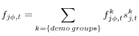
where ![]() is the share of job type j that is of demographic group k (i.e.
is the share of job type j that is of demographic group k (i.e.
![]() ).
).
The change in the aggregate flow between t and t-1 is: 8)
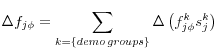 Each component of the sum is that demographic group's contribution to the change
in the aggregate flow. For each demographic group k, note that: 9)
Each component of the sum is that demographic group's contribution to the change
in the aggregate flow. For each demographic group k, note that: 9)
![]() where bars above the flow or share indicate the average share or
flow rate for that demographic group over the relevant period. Dividing (9) by (8), i.e. by the total change in the flow over this period, represents the share of the change in the flow attributable to group k. Multiplying by 100, this is the shaded column in each panel
of table 5. Dividing the first term in the summation of (9) by (8), and multiplying by 100, is the percent change in the aggregate flow attributable to group k's change in their group-flow rate (the second column of each panel); and dividing the second term of (9) by the
total flow is the change in the aggregate flow attributable to the change of group k's employment share.
where bars above the flow or share indicate the average share or
flow rate for that demographic group over the relevant period. Dividing (9) by (8), i.e. by the total change in the flow over this period, represents the share of the change in the flow attributable to group k. Multiplying by 100, this is the shaded column in each panel
of table 5. Dividing the first term in the summation of (9) by (8), and multiplying by 100, is the percent change in the aggregate flow attributable to group k's change in their group-flow rate (the second column of each panel); and dividing the second term of (9) by the
total flow is the change in the aggregate flow attributable to the change of group k's employment share.
So, of the four flows that appear most relevant for understanding the dynamics of labor market polarization:
- Declining inflow rate to middle-type from non-employment: Nearly half of the decline is attributable to the decline in the inflow rate of 16-24 year olds. Most of the rest can be explained by a declining inflow and employment share for non-college females.
- Rising outflow rate from middle-type to non-middle-type: 40 percent is explainable by 55+ (due equally to a rising employment share and an increase in their transition rate), while rising outflow rates for prime-age males and females of all education types also contribute.
- Rising inflow rate from non-low-type to low-type: Rising within-group transition rates (particularly among the young and less educated) explain much of this trend, while composition shifts (declining employment share of the young and less educated) work against it.
- Rising inflow rate from non-high-type to high-type: Most of this increase is attributable to an increase in the college-share of the employed population (the college-educated are more likely to make transitions of this type). Also, the inflow rate within-groups has also increased over this period, particularly for those aged 55 and older, though it has also increased modestly within most other demographic groups.
So to summarize, it seems that since the mid-1980s, much of the observed labor market polarization is attributable to: declining transition rates from non-employment to middle-type jobs, particularly for the young and less educated; rising outflow rates from middle-type jobs to other jobs (within all demographic groups); rising inflow rates to high-type jobs from non-high type jobs, in part because of the rising employment share of the college-educated and also because of rising inflow rates within most demographic groups; and rising inflow rates to low-type jobs from non-low type jobs within all demographic groups.
5. The contribution of changing inflow/outflow rates to polarization around recessions
Finally, I return to addressing how inflow and outflow rates have changed around recent recessions, and how changes in these rates have mechanically affected the share of employment by job-type (using a similar decomposition as described in the earlier sections). Recall from Table 2 that the share of employment in middle-type jobs declined significantly following the 1990 and 2001 recessions, and failed to recover. Armed with a framework for analyzing flow rates and their contribution to employment shares, I estimate changes in the 12-month moving average of the four one-month and twelve-month transition rates, and the change in counterfactual steady states formed by holding the flow rates at their 12 month pre-recession average (table 6).
Some observations regarding the decline in middle-type employment surrounding the recessions:
- 1990 recession: The decline in middle-type employment appears primarily due to a decline in the inflow rate from non-employment (one- and twelve-month transition rates) .
- 2001 recession: The "explanation" behind the decline in middle-type employment depends in part on the transition horizon considered. Steady-state counterfactuals formed using one-month transition rates suggest that a decline in inflow rates (from non-employment and non-middle-type jobs) are most important. Counterfactuals formed using twelve-month transition rates suggest that an increase in outflow rates (to other job types, and non-employment) are most important.
- 2008 recession: The most striking observation regarding the 2008 recession is that for all job types: outflow rates to non-employment (twelve-month transitions) increased, outflow rates to other types of employment fell (and thus the inflow rate from other job types also fell), and that inflow rates from non-employment also declined. Regarding the decline in middle-type employment, using twelve-month transition rates the increase in the outflow rate to non-employment, and decline in the inflow rate from other employment and non-employment all appear important.
To summarize, one consistent "explanation" for the decline in the share employed in middle-type jobs following the last three recessions, at least based on a steady-state counterfactual analysis using twelve-month transition rates, is because of an increase in outflow rates to non-employment. It also appears that a decline in inflow rates is also important for explaining the decline in middle-type employment in the 1991 and 2008 episodes. The relative importance of changes in inflow and outflow rates surrounding the 2001 episode depends on whether the steady states are formed using one- or twelve-month transition rates. Regardless, this analysis suggests that both changes in inflow and outflow rates contribute, though the relative degree to which inflow and outflow rates are important may vary depending on the episode. One implication is that any theory about how the labor market cycle interacts with polarization and other structural changes must consider changes to transitions both into and out of middle-type jobs (and, given the different relative importance of inflow and outflow rates around these episodes, there may not be a single unifying explanation).
V.Conclusion
This paper uses data from a number of sources to examine the flow of workers and the non-employed between jobs of different types. In doing so, it is the most detailed exploration to-date into the labor market dynamics behind polarization. Using matched monthly CPS data (forming one-, four-, eight-, and twelve-month job transitions), data from the March CPS Supplement, and Displaced Worker Survey data, I have shown that trends in inflow and outflow rates are both important for understanding the mechanics behind why the aggregate share of workers is declining in middle-type jobs and rising in low- and high-type jobs. For instance, it appears that since the mid-1980s, the decline in inflows to middle-type jobs from non-employment and the increase in outflows from middle-type to other jobs (and non-employment) are both important for explaining why employment shares in middle-type jobs have fallen. Also, a large share of the decline in inflows from non-employment appears attributable to 16-24 year olds, suggesting that this phenomenon may be linked to the ongoing decline in youth employment and participation rates (e.g. Smith 2011). Regarding the decline in middle-type employment surrounding recent recessions, discrete changes in both inflow and outflow rates also appear to be important. These findings, as well as the broader evidence for the last 25 years, suggest that any theory linking polarization to weak labor market performance must accommodate the fact that trends in aggregate inflow and outflow rates to and from middle-type jobs are all of significant importance.
Although this paper goes the furthest yet towards understanding what happens to workers who are displaced from middle-type jobs, and more generally the labor market dynamics behind polarization, there are many related and important questions that remain unanswered. For instance, what happens to displaced middle-type workers at horizons longer than those captured in matched CPS data or the Displaced Worker Survey? Of the former middle-type workers who increasingly remain non-employed (Figure 6), what fraction of these eventually re-enter the workforce, and what fraction remain permanently displaced (perhaps by moving onto disability insurance rolls)?
One primary finding of this research is that the decline in inflow rates into middle-type jobs important for understanding polarization, and much of this decline is due to younger adults. The welfare and policy implications of this finding therefore depend on where these workers who would have been in middle-type employment are going. To the extent that they are receiving greater amounts of education, increasingly working in high-type jobs and receive higher lifetime earnings, then this aspect of polarization may be a positive development. However, this is surely not the case for all workers displaced from middle-type jobs or who would have worked in these jobs had such jobs been available. For instance, some younger workers may be finding themselves stuck in low-type employment (their outflow rate from low-type jobs to other types has fallen), and non-college adults may be increasingly finding themselves displaced into low-type jobs (their inflow rate to low-type jobs from other types of employment has increased significantly more than for the college-educated population). These aspects of polarization perhaps raise more troubling questions about the longer-run labor market performance of these sorts of workers, and require further research and attention.
References
Abel, Jaison R. and Richard Deitz. 2012. "Job Polarization and Rising Inequality in the Nation and the New York-Northern New Jersey Region." Current Issues in Economics and Finance, Federal Reserve Bank of New York, 18(7).
Acemoglu, Daron and David Autor. 2011. "Skills, Tasks and Technologies: Implications for Employment and Earnings." In Handbook of Labor Economics Volume 4, Orley Ashenfelter and David E. Card (eds). Amsterdam: Elsevier, 2011.
Albanesi, Stefania, Victoria Gregory, Christina Patterson, and Aysegul Sahin. March 27, 2013. "Is Job Polarization Holding Back the Labor Market?" Liberty Street Economics blog, Federal Reserve Bank of New York. http://libertystreeteconomics.newyorkfed.org/2013/03/is-job-polarization-holding-back-the-labor-market.html
Autor, David. 2010. "The Polarization of Job Opportunities in the U.S. Labor Market: Implications for Employment and Earnings." Center for American Progress and The Hamilton Project.
Autor, David, Frank Levy, and Richard J. Murnane. 2003. "The Skill Content of Recent Technological Change: An Empirical Exploration." Quarterly Journal of Economics. 118(4), 1279-1333.
Autor, David, Lawrence Katz, and Melissa Kearney. 2006. "The Polarization of the U.S. Labor Market." American Economic Review Papers and Proceedings. 96(2): 189-194.
Autor, David and David Dorn. 2009. "This Job is "Getting Old": Measuring Changes in Job Opportunities using Occupational Age Structure." American Economic Review: Papers and Proceedings. 99(2), 45-51.
Autor, David and David Dorn. 2013. "The Growth of Low Skill Service Jobs and the Polarization of the U.S. Labor Market." American Economic Review, forthcoming.
Autor, David, David Dorn, and Gordon Hanson. 2013a. "The China Syndrome: Local Labor Market Effects of Import Competition in the United States." American Economic Review, forthcoming.
Autor, David, David Dorn, and Gordon Hanson. 2013b. "Untangling Trade and Technology: Evidence from Local Labor Markets." Unpublished mimeo.
Barnichon, Regis and Christopher J. Nekarda. 2012. "The Ins and Outs of Forecasting Unemployment: Using Labor Force Flows to Forecast the Labor Market." Brookings Papers on Economic Activity, Fall 2012, 83-131.
Beaudry, Paul, David A. Green, and Ben Sand. 2013. "The Great Reversal in the Demand for Skill and Cognitive Tasks." NBER Working Paper No. 18901, March 2013.
Charles, Kerwin Kofi, Erik Hurst, and Matthew J. Notowidigdo. 2013. "Manufacturing Decline, Housing Booms, and Non-employment." National Bureau of Economic Research Working Paper No. 18949, April.
Goos, Maarten and Alan Manning. 2007. "Lousy and Lovely Jobs: The Rising Polarization of Work in Britain." Review of Economics and Statistics, 89(1), 118-133.
Foote, Christopher L. and Richard W. Ryan. 2012. "Labor-Market Polarization Over the Business Cycle." Federal Reserve Bank of Boston Public Policy Discussion Papers, No. 12-8.
Jaimovich, Nir and Henry E. Sui. 2012. "The Trend is the Cycle: Job Polarization and Jobless Recoveries." NBER Working Paper No. 18334. August 2012.
Manning, Alan, Maarten Goos and Anna Salomons. 2011. "Explaining Job Polarization in Europe: The Role of Technology, Globalization and Institutions." Unpublished mimeo.
Manning, Alan, Maarten Goos and Anna Salomons. 2009. "Job Polarization in Europe." American Economic Review Papers and Proceedings, 99(2), 58-63.
Mazzolari, Francesca and Giuseppe Ragusa. 2013. "Spillovers from High-Skill Comsumption to Low-Skill Labor Markets." Review of Economics and Statistics, forthcoming.
Michaels, Guy, Ashwini Natraj, and John Van Reenen. 2013. "Has ICT Polarized Skill Demand? Evidence from Eleven Countries over 25 Years." Review of Economics and Statistics, forthcoming.
Moscarini, Giuseppe and Kaj Thomsson. 2007. "Occupational and Job Mobility in the US." Scandinavian Journal of Economics. 109(4), 807-836.
National Employment Law Project. 2012. "The Low-Wage Recovery and Growing Inequality." Data Brief, August 2012.
Smith, Christopher. 2011. "Polarization, Immigration, Education: What's Behind the Dramatic Decline in Youth Employment?" Finance and Economics Discussion Series, 2011-41. Board of Governors of the Federal Reserve System.
Shimer, Robert. 2012. "Reassessing the Ins and Outs of Unemployment." Review of Economic Dynamics, 15(2): 127-148.
Spitz-Oener, Alexandra. 2006. "Technical Change, Job Tasks, and Rising Educational Demands: Looking outside the Wage Structure." Journal of Labor Economics. 24(2), 235-270.
Tuzemen, Didem and Jonathan Willis. 2013. "The Vanishing Middle: Job Polarization and Workers' Response to the Decline in Middle-Skill Jobs." Economic Review, 2013 Q1. Federal Reserve Bank of Kansas City.
Note: Plots 12 month moving average of the share of the 16+ population working in the listed occupation (or nonemployed, the black line in panel A). Constructed from monthly CPS data
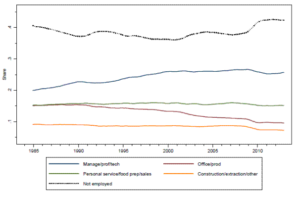
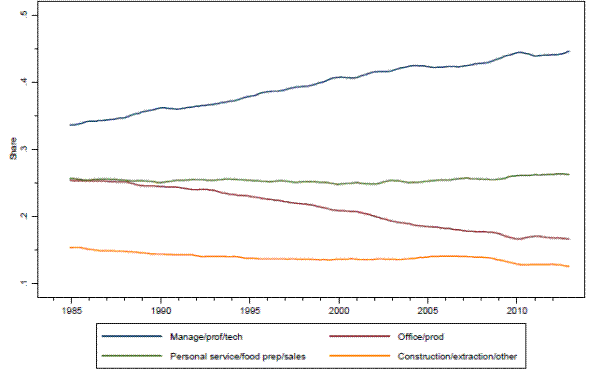
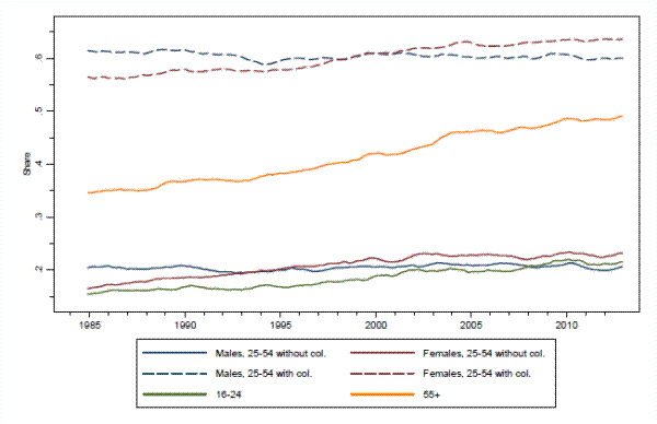
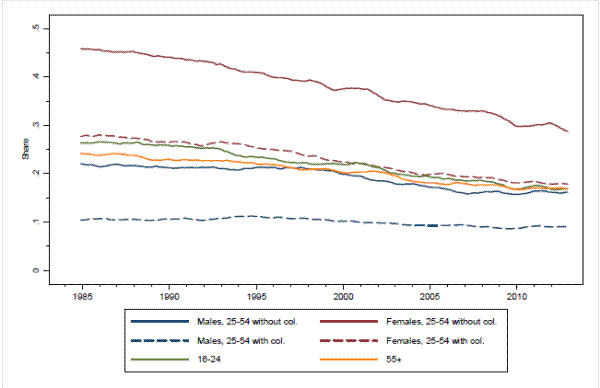
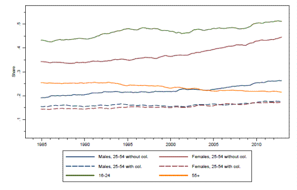
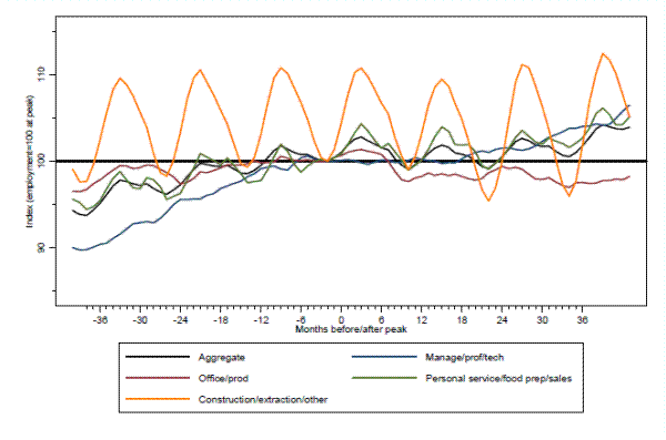
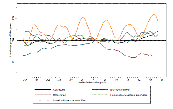
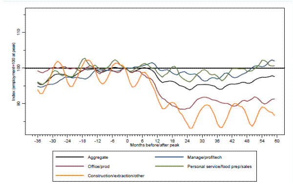
Figure 4: Monthly transition rates, cond. on being unemp. in prev. month (monthly CPS data)
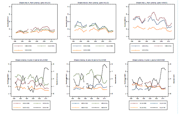 Figure 4 Data
Figure 5: Monthly transition rates, cond. on being unemp. in prev. month, by duration of unemp. (monthly CPS data)
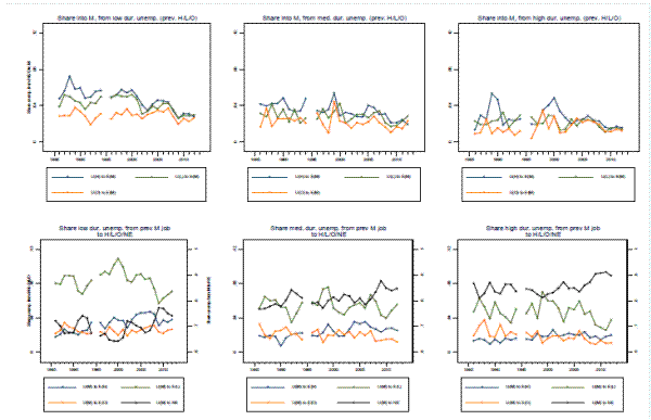 Figure 5 Data
Figure 6 :Monthly transition rates, cond. on being unemp. 1-12 months previously (monthly CPS data)
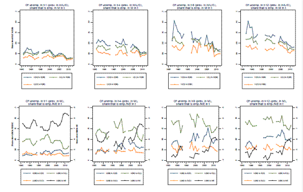 Figure 6 Data
Figure 7: Transition rates from displaced occupation, cond. on being displaced in last three years (displaced worker survey)
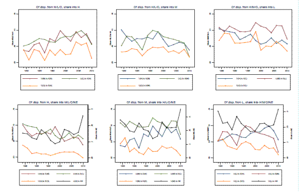 Figure 7 Data
Figure 8: Monthly transition rates, uncond. on prev. month's emp. status (monthly CPS data)
 Figure 8 Data
Figure 9A: Short and long transition rates, to and from high-type jobs (CPS monthly data)
 Figure 9a Data
Figure 9B: Short and long transition rates, to and from middle-type jobs (CPS monthly data)
 Figure 9b Data
Figure 9C: Short and long transition rates, to and from low-type jobs (CPS monthly data)
 Figure 9c Data
Figure 10: Annual transition rates, uncond. on employment status in prev. year (March CPS )
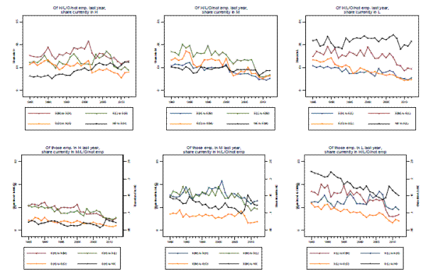 Figure 10 Data
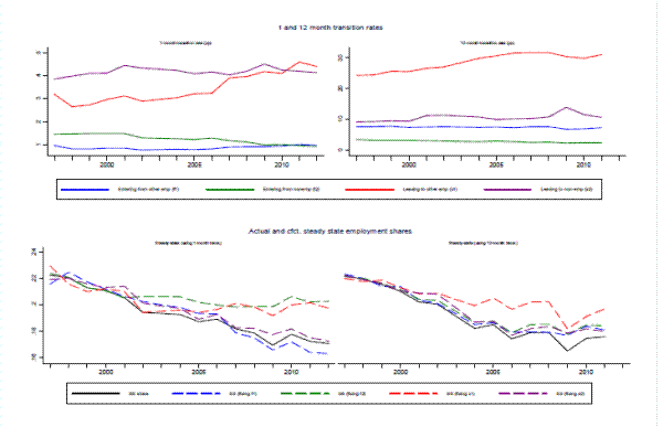
Table 1: Characteristics of jobs by type (1985-1987)
| Included occupations: | High-type, Professional managerial technical | Middle-type, Non-sup. prod. and office | Low-type, Personal service food prep. sales | Other, Constr. extract. repair transp. material moving farming |
|---|---|---|---|---|
| Average hourly wage (2012 dollars) | 25.6 | 16.4 | 13.7 | 18.3 |
| Average weekly wage (2012 dollars) | 1042.5 | 631.7 | 505.4 | 752.2 |
| Average weekly hours | 40.8 | 37.7 | 34.4 | 40.8 |
| Average age | 39.3 | 37.2 | 35.4 | 37.7 |
| Fraction of employment in top 50% of most intensively non-routine cognitive jobs | 0.97 | 0.34 | 0.38 | 0.54 |
| Fraction of employment in top 50% of most intensively routine jobs | 0.26 | 0.86 | 0.36 | 0.71 |
| Fraction of employment in top 50% of most intensively non-routine manual jobs | 0.53 | 0.30 | 0.59 | 0.88 |
| For each job type share that is1: Male | 0.56 | 0.38 | 0.51 | 0.93 |
| For each job type share that is1:No high school degree | 0.03 | 0.15 | 0.24 | 0.28 |
| For each job type share that is1:Bachelor's degree or better | 0.57 | 0.09 | 0.12 | 0.05 |
| For each job type share that is1: 16-24 both sexes | 0.08 | 0.18 | 0.29 | 0.17 |
| For each job type share that is1:Males 25-54 no college | 0.08 | 0.18 | 0.16 | 0.49 |
| For each job type share that is1:Males 25-54 at least some coll. | 0.36 | 0.09 | 0.14 | 0.15 |
| For each job type share that is1: Females 25-54 no college | 0.08 | 0.28 | 0.20 | 0.03 |
| For each job type share that is1:Females 25-54 at least some coll. | 0.27 | 0.14 | 0.08 | 0.01 |
| For each job type share that is1: 55+ both sexes | 0.13 | 0.13 | 0.13 | 0.14 |
| For each demographic group share of employed that is of given type2: 16-24 both sexes | 0.12 | 0.27 | 0.46 | 0.15 |
| For each demographic group share of employed that is of given type2:Males 25-54 no college | 0.11 | 0.25 | 0.24 | 0.40 |
| For each demographic group share of employed that is of given type2: Males 25-54 at least some coll. | 0.53 | 0.12 | 0.22 | 0.13 |
| For each demographic group share of employed that is of given type2:Females 25-54 no college | 0.13 | 0.47 | 0.37 | 0.03 |
| For each demographic group share of employed that is of given type2: Females 25-54 at least some coll. | 0.54 | 0.27 | 0.17 | 0.01 |
| For each demographic group share of employed that is of given type2: 55+ both sexes | 0.27 | 0.26 | 0.30 | 0.17 |
1 - For bottom 6 rows of panel each column adds to 1. 2 - Each row adds to 1.
Table 2: Change in employment and employment shares surrounding recessions
| Change in # employed (pct): All | Change in # employed (pct): High | Change in # employed (pct): Middle | Change in # employed (pct): Low | Change in # employed (pct): Other | Change in share of employed (pp): High | Change in share of employed (pp): Middle | Change in share of employed (pp): Low | Change in share of employed (pp): Other | |
|---|---|---|---|---|---|---|---|---|---|
| All: 1990/91 recession (change in twelve-month MA, March 1990 to March 1992) | -0.1 | 0.8 | -1.6 | 1.2 | -2.2 | 0.3 | -0.4 | 0.3 | -0.3 |
| All: 16-24 (1990/91 recession:change in twelve-month MA, March 1990 to March 1992) | -5.8 | -9.7 | -7.1 | -1.1 | -13.5 | -0.7 | -0.3 | 2.2 | -1.1 |
| All: Males 25-54 no coll. (1990/91 recession:change in twelve-month MA, March 1990 to March 1992) | -1.3 | -6.6 | -0.8 | 3.6 | -1.5 | -1.1 | 0.1 | 1.0 | -0.1 |
| All: Males 25-54 w/ coll. (1990/91 recession:change in twelve-month MA, March 1990 to March 1992) | 3.0 | 1.7 | 1.9 | 6.5 | 6.1 | -0.8 | -0.1 | 0.5 | 0.4 |
| All: Females 25-54 no coll.(1990/91 recession:change in twelve-month MA, March 1990 to March 1992) | -0.8 | 1.4 | -2.5 | 0.4 | -2.7 | 0.4 | -0.8 | 0.4 | -0.1 |
| All:Females 25-54 w/coll.(1990/91 recession:change in twelve-month MA, March 1990 to March 1992) | 6.4 | 6.9 | 4.0 | 8.3 | 12.4 | 0.3 | -0.6 | 0.3 | 0.1 |
| All: 55+ (1990/91 recession:change in twelve-month MA, March 1990 to March 1992) | -3.0 | -3.0 | -3.4 | -2.4 | -3.5 | 0.0 | -0.1 | 0.2 | -0.1 | All: (2001 recession: change in twelve-month MA March 2001 to March 2003) | -0.2 | 2.3 | -7.1 | 1.2 | 0.2 | 1.0 | -1.4 | 0.4 | 0.1 |
| All: 16-24 (2001 recession: change in twelve-month MA March 2001 to March 2003) | -5.0 | 0.3 | -14.2 | -2.7 | -5.0 | 1.1 | -2.1 | 1.0 | 0.0 |
| All: Males 25-54 no coll. (2001 recession: change in twelve-month MA March 2001 to March 2003) | -1.7 | 2.8 | -8.9 | -2.1 | -0.3 | 0.9 | -1.4 | -0.1 | 0.6 |
| All: Males 25-54 w/ coll. (2001 recession: change in twelve-month MA March 2001 to March 2003) | -2.0 | -3.5 | -1.5 | 3.0 | -1.6 | -0.9 | 0.0 | 0.8 | 0.1 |
| All: Females 25-54 no coll. (2001 recession: change in twelve-month MA March 2001 to March 2003) | -5.2 | 3.8 | -13.5 | -2.8 | 2.1 | 2.1 | -3.3 | 0.9 | 0.3 |
| All: Females 25-54 w/coll. (2001 recession: change in twelve-month MA March 2001 to March 2003) | 0.1 | 0.6 | -5.7 | 6.2 | 1.0 | 0.3 | -1.3 | 0.9 | 0.0 |
| All: 55+ (2001 recession: change in twelve-month MA March 2001 to March 2003) | 12.0 | 17.9 | 6.5 | 10.4 | 5.0 | 2.2 | -1.0 | -0.3 | -0.9 |
| All (2008 recession: change in twelve-month MA, Dec. 2007 to Dec. 2009) | -4.2 | -0.7 | -9.9 | -2.5 | -11.0 | 1.6 | -1.1 | 0.5 | -1.0 |
| All: 16-24 (2008 recession: change in twelve-month MA, Dec. 2007 to Dec. 2009) | -11.3 | -5.8 | -19.2 | -7.2 | -24.2 | 1.4 | -1.7 | 2.1 | -1.8 |
| All: Males 25-54 no coll. (2008 recession: change in twelve-month MA, Dec. 2007 to Dec. 2009) | -9.6 | -8.1 | -11.6 | -4.4 | -12.9 | 0.4 | -0.4 | 1.4 | -1.4 |
| All:Males 25-54 w/ coll. (2008 recession: change in twelve-month MA, Dec. 2007 to Dec. 2009) | -4.5 | -3.8 | -7.2 | -1.0 | -9.9 | 0.5 | -0.3 | 0.6 | -0.8 |
| All: Females 25-54 no coll. (2008 recession: change in twelve-month MA, Dec. 2007 to Dec. 2009) | -8.0 | -2.7 | -16.8 | -4.8 | -5.9 | 1.4 | -2.9 | 1.4 | 0.1 |
| All:Females 25-54 w/coll. (2008 recession: change in twelve-month MA, Dec. 2007 to Dec. 2009) | -0.8 | -0.1 | -5.8 | 3.0 | -6.9 | 0.4 | -1.0 | 0.7 | -0.1 |
| All:55+ (2008 recession: change in twelve-month MA, Dec. 2007 to Dec. 2009) | 5.5 | 9.3 | 0.1 | 4.0 | 1.8 | 1.7 | -0.9 | -0.3 | -0.4 |
Note: First five columns display the percent change in the 12 month trailing moving average of the number of the given demographic group employed in the given occupation. The last four columns display the change (in percentage points) of the share of the demographic group employed in the given occupations conditional on being employed.
Table 3: Contrib. of changes in 1-month and 12-month transition rates to changes in employment shares (1997-99 to 2009-11)
| High-type | Middle-type | Low-type | Other-type | |
|---|---|---|---|---|
| Change in share (pp): Actual uncond. | 0.1 | -3.9 | -0.8 | -1.2 |
| Change in share (pp): Actual cond. | 4.1 | -4.6 | 1.2 | -0.7 |
| A. 1-month transition rates: Change in 1-month transition rate (pp): Inflow rate from other emp. | 0.7 | 0.1 | 0.4 | 0.1 |
| A. 1-month transition rates: Change in 1-month transition rate (pp):Inflow rate from non-emp. | 0.3 | -0.4 | -0.6 | -0.2 |
| A. 1-month transition rates: Change in 1-month transition rate (pp): Outflow rate to other emp. | 0.6 | 1.6 | 0.5 | 0.9 |
| A. 1-month transition rates: Change in 1-month transition rate (pp):Outflow rate to non-emp. | 0.6 | 0.5 | -0.2 | 1.1 |
| A. 1-month transition rates: Change in within-sample share cond. (pp) | 4.0 | -4.6 | 1.2 | -0.7 |
| A. 1-month transition rates: Change in within-sample share cond. (pp): Steady state share | 4.6 | -5.4 | 1.8 | -1.0 |
| A. 1-month transition rates: Change in within-sample share cond. (pp): Fixing inflow rate from other emp. | 1.3 | -5.9 | 0.1 | -1.9 |
| A. 1-month transition rates: Change in within-sample share cond. (pp): Fixing inflow rate from non-emp. | 2.7 | -2.7 | 4.4 | 0.1 |
| A. 1-month transition rates: Change in within-sample share cond. (pp): Fixing outflow rate to other emp. | 6.9 | -2.8 | 2.6 | -0.1 |
| A. 1-month transition rates: Change in within-sample share cond. (pp): Fixing outflow rate to non-emp. | 7.1 | -4.5 | 1.5 | 0.2 |
| B. 12-month transition rates: Change in 12-month transition rate (pp): Inflow rate from other emp. | 2.4 | -0.6 | 1.2 | 0.2 |
| B. 12-month transition rates: Change in 12-month transition rate (pp):Inflow rate from non-emp. | 0.4 | -1.0 | -1.0 | -0.0 |
| B. 12-month transition rates: Change in 12-month transition rate (pp): Outflow rate to other emp. | 0.8 | 5.6 | -1.5 | 2.1 |
| B. 12-month transition rates: Change in 12-month transition rate (pp): Outflow rate to non-emp. | 1.9 | 2.8 | 1.5 | 4.3 |
| B. 12-month transition rates: Change in within-sample share cond. (pp) | 3.8 | -4.8 | 1.8 | -0.9 |
| B. 12-month transition rates: Change in steady state share (cond. on emp.):Steady state share | 2.7 | -4.7 | 3.0 | -1.0 |
| B. 12-month transition rates: Change in steady state share (cond. on emp.):Fixing inflow rate from other emp. | 0.4 | -3.9 | 1.8 | -1.3 |
| B. 12-month transition rates: Change in steady state share (cond. on emp.):Fixing inflow rate from non-emp. | 2.3 | -3.7 | 3.9 | -0.9 |
| B. 12-month transition rates: Change in steady state share (cond. on emp.):Fixing outflow rate to other emp. | 3.4 | -2.9 | 2.5 | -0.4 |
| B. 12-month transition rates: Change in steady state share (cond. on emp.):Fixing outflow rate to non-emp. | 4.3 | -3.9 | 3.6 | 0.2 |
Note: In the top two rows is summarized the change in the share of the given population employed in high, middle, or low-type occupations, conditional and unconditional on being employed. For each panel, in the top four rows is summarized the inflow and outflow transition rates from the given job type based on one-month (panel A) or twelve-month (panel B) transition rates as calculated in the CPS. For each panel, in the bottom four rows are summarized change in shares calculated for the sample used to make the transition rates, the steady state shares consistent with the transition rates, as well as counterfactual steady states that are formed by holding each of the four transition rates (independently) at their 1997-1999 average flow rate.
Table 4: Changes in avg. 12-month trans. rates and contrib. of trans. rates to changes in emp. shares (1987-89 to 2009-11)
| All | 16-24 | Males: 25-54 no col. | Males: 25-54 w/ col. | Females: 25-54 no col. | Females: 25-54 w/ col. | 55+ | |
|---|---|---|---|---|---|---|---|
| A. High-type Change in share (pp):Actual uncond. | 3.5 | -0.3 | -2.4 | -5.4 | 1.8 | 3.3 | 7.2 |
| A. High-type Change in share (pp):Actual cond. | 8.7 | 5.0 | -0.0 | -1.2 | 4.6 | 6.1 | 12.4 |
| A. High-type Change in share (pp):Within-samp cond. | 8.3 | 4.9 | -0.9 | -2.5 | 4.3 | 3.6 | 12.5 |
| A. High-type Change in avg. 12-month transition rate (pp):Inflow rate from other emp. | 4.4 | 1.9 | 1.2 | 1.1 | 2.2 | 3.4 | 6.2 |
| A. High-type Change in avg. 12-month transition rate (pp):Inflow rate from non-emp. | 0.9 | -0.1 | -0.9 | -5.1 | 0.1 | 0.7 | 0.6 |
| A. High-type Change in avg. 12-month transition rate (pp):Outflow rate to other emp. | 0.6 | -2.5 | 4.7 | 1.7 | 1.7 | 1.0 | 0.6 |
| A. High-type Change in avg. 12-month transition rate (pp):Outflow rate to non-emp. | 2.0 | 5.6 | 3.8 | 1.8 | 1.6 | 0.1 | -0.9 | A. High-type Change in steady state share (cond. on emp.):Steady state share | 7.0 | 4.1 | -1.6 | -2.9 | 2.8 | 3.1 | 12.7 |
| A. High-type Change in steady state share (cond. on emp.): Fixing inflow rate from other emp. | 2.4 | 1.9 | -3.3 | -3.6 | -0.2 | 1.5 | 7.0 |
| A. High-type Change in steady state share (cond. on emp.):Fixing inflow rate from non-emp. | 5.9 | 4.1 | -0.9 | -2.3 | 2.8 | 2.9 | 9.0 |
| A. High-type Change in steady state share (cond. on emp.):Fixing outflow rate to other emp. | 7.5 | 3.1 | 0.6 | -1.2 | 3.5 | 3.6 | 13.1 |
| A. High-type Change in steady state share (cond. on emp.): Fixing outflow rate to non-emp. | 8.6 | 6.1 | 0.2 | -1.2 | 3.5 | 3.4 | 12.1 |
| B. Middle-type Change in share (pp): Actual uncond. | -5.6 | -8.1 | -6.5 | -2.1 | -10.4 | -7.2 | -0.6 |
| B. Middle-type Change in share (pp):Actual cond. | -7.9 | -9.0 | -5.4 | -1.6 | -14.5 | -8.7 | -6.3 |
| B. Middle-type Change in share (pp): Within-samp cond. | -8.0 | -9.5 | -5.4 | -0.7 | -15.3 | -6.4 | -6.1 |
| B. Middle-type Change in avg. 12-month transition rate (pp): Inflow rate from other emp. | -0.6 | -4.2 | 0.2 | 0.6 | -2.6 | -0.0 | 0.6 |
| B. Middle-type Change in avg. 12-month transition rate (pp): Inflow rate from non-emp. | -1.4 | -4.3 | -2.8 | -4.1 | -3.6 | -2.9 | -0.0 |
| B. Middle-type Change in avg. 12-month transition rate (pp): Outflow rate to other emp. | 10.3 | 10.2 | 7.6 | 8.3 | 9.4 | 7.6 | 10.6 |
| B. Middle-type Change in avg. 12-month transition rate (pp): Outflow rate to non-emp. | 2.4 | 4.2 | 5.2 | 2.7 | 2.2 | 0.9 | -0.8 |
| B. Middle-type Change in steady state share (cond. on emp.): Steady state share | -8.2 | -11.3 | -4.5 | -0.6 | -17.2 | -5.8 | -6.0 |
| B. Middle-type Change in steady state share (cond. on emp.):Fixing inflow rate from other emp. | -7.4 | -7.1 | -4.8 | -1.7 | -14.3 | -5.8 | -6.9 |
| B. Middle-type Change in steady state share (cond. on emp.): Fixing inflow rate from non-emp. | -6.7 | -8.2 | -3.1 | 0.0 | -14.3 | -4.8 | -5.8 |
| B. Middle-type Change in steady state share (cond. on emp.):Fixing outflow rate to other emp. | -4.5 | -8.3 | -1.9 | 0.9 | -11.5 | -2.7 | -2.0 |
| B. Middle-type Change in steady state share (cond. on emp.):Fixing outflow rate to non-emp. | -7.5 | -10.3 | -2.8 | -0.2 | -16.1 | -5.5 | -6.2 |
| C. Low-type Change in share (pp): Actual uncond. | -0.5 | -3.7 | 1.6 | 0.4 | 3.9 | 1.6 | 0.7 |
| C. Low-type Change in share (pp): Actual cond. | 0.9 | 6.9 | 5.4 | 1.7 | 9.4 | 2.6 | -3.4 |
| C. Low-type Change in share (pp): Within-samp cond. | 1.3 | 6.9 | 5.2 | 1.9 | 10.1 | 2.6 | -3.2 |
| C. Low-type Change in avg. 12-month transition rate (pp): Inflow rate from other emp. | 1.3 | 4.2 | 3.0 | 1.1 | 4.6 | 1.0 | 0.9 |
| C. Low-type Change in avg. 12-month transition rate (pp): Inflow rate from non-emp. | -1.0 | -6.2 | -2.2 | -2.8 | -1.4 | -0.7 | -0.1 |
| C. Low-type Change in avg. 12-month transition rate (pp): Outflow rate to other emp. | -0.1 | -6.0 | -0.9 | 0.2 | -1.8 | -0.6 | 5.0 |
| C. Low-type Change in avg. 12-month transition rate (pp): Outflow rate to non-emp. | 0.5 | 4.1 | 4.5 | 2.8 | -1.5 | -1.9 | -2.0 |
| C. Low-type Change in steady state share (cond. on emp.): Steady state share | 2.6 | 9.2 | 5.5 | 2.4 | 11.9 | 2.7 | -4.8 |
| C. Low-type Change in steady state share (cond. on emp.): Fixing inflow rate from other emp. | 1.2 | 7.6 | 2.2 | 0.5 | 8.9 | 1.6 | -6.0 |
| C. Low-type Change in steady state share (cond. on emp.): Fixing inflow rate from non-emp. | 3.4 | 11.4 | 6.4 | 2.9 | 12.6 | 2.9 | -4.3 |
| C. Low-type Change in avg. 12-month transition rate (pp): Fixing outflow rate to other emp. | 2.5 | 7.4 | 5.3 | 2.6 | 11.1 | 2.3 | -2.7 |
| C. Low-type Change in avg. 12-month transition rate (pp): Fixing outflow rate to non-emp. | 2.7 | 10.5 | 7.1 | 3.3 | 11.2 | 2.3 | -5.5 |
Note: In the first three rows of each panel is summarized the change in the share of the given population employed in high, middle, or low-type occupations, conditional and unconditional on being employed for the whole sample, and (in the third row) for the sample that can be matched month-to-month in the CPS. In the middle four rows is summarized the 12-month inflow and outflow transition rates for the given job type as calculated in the CPS. In the bottom four rows are summarized the steady state shares consistent with the 12-month transition rates, as well as counterfactual steady states that are formed by holding each of the four transition rates (independently) at their 1987-1989 average.
Table 5: Decomposition of changes in flows, by demographics (1987-1989 to 2009-2011). Contributions to change in flows from each group:Total contrib, contrib from change in 12 month trans rate, and contrib from change in each group's pop. share.
| Total change (in pp.) | 16-24, Contrib (pct of total) | 16-24, Contrib flow (pct) | 16-24, Contrib share (pct) | Males, 25-54 no college, Contrib (pct of total) | Males, 25-54 no college, Contrib flow (pct) | Males, 25-54 no college, Contrib share (pct) | Males, 25-54 w/ college, Contrib (pct of total) | Males, 25-54 w/ college, Contrib flow (pct) | Males, 25-54 w/ college, Contrib share (pct) | Females, 25-54 no college, Contrib (pct of total) | Females, 25-54 no college, Contrib flow (pct) | Females, 25-54 no college, Contrib share (pct) | Females, 25-54 w/ college, Contrib (pct of total) | Females, 25-54 w/ college, Contrib flow (pct) | Females, 25-54 w/ college, Contrib share (pct) | 55+, Contrib (pct of total) | 55+, Contrib flow (pct) | 55+, Contrib share (pct) | |
|---|---|---|---|---|---|---|---|---|---|---|---|---|---|---|---|---|---|---|---|
| Change in avg. 12-month transition: High-type: Inflow rate from other emp. | 4.4 | -0.8 | 6.6 | -7.4 | -3.7 | 6.6 | -10.1 | 25.4 | 3.5 | 21.9 | -9.9 | 9.5 | -19.4 | 37.0 | 10.1 | 26.9 | 52.1 | 32.0 | 20.1 |
| Change in avg. 12-month transition: High-type: Inflow rate from non-emp. | 0.9 | 10.1 | -1.044458 | 11.3 | 0.7 | -4.8 | 5.2 | 26.7 | -14.4 | 41.0 | -13.3 | 1.1 | -14.3 | 37.1 | 5.5 | 31.1 | 38.7 | 41.1 | -2.2 |
| Change in avg. 12-month transition: High-type: Outflow rate to other emp. | 0.6 | 127.7 | 37.5 | 87.8 | 504.1 | -175.7 | 676.2 | 12.5 | -215.1 | 225.8 | 408.0 | -44.6 | 452.5 | -352.4 | -109.9 | -242.7 | -599.8 | -52.9 | -548.4 |
| Change in avg. 12-month transition: High-type: Outflow rate to non-emp. | 2.0 | 4.5 | 11.4 | -6.2 | 4.4 | 19.3 | -14.8 | 24.3 | 32.2 | -7.9 | -10.7 | 5.7 | -16.5 | 19.3 | 1.8 | 17.5 | 58.3 | -10.8 | 69.0 |
| Middle-type: Inflow rate from other emp. | -0.6 | 90.3 | 49.1 | 40.6 | 51.4 | -3.6 | 55.0 | -18.8 | -16.7 | -2.2 | 101.0 | 30.8 | 70.5 | -54.1 | 0.5 | -54.8 | -69.8 | -15.7 | -54.1 |
| Middle-type: Inflow rate from non-emp. | -1.4 | 33.9 | 46.1 | -10.8 | 4.2 | 9.5 | -5.3 | -2.0 | 7.6 | -9.8 | 56.7 | 30.7 | 26.3 | 4.4 | 16.5 | -12.0 | 2.8 | 1.9 | 1.0 |
| Middle-type::Outflow rate to other emp. | 10.3 | 1.4 | 10.4 | -9.2 | -1.2 | 12.2 | -13.3 | 22.2 | 7.9 | 14.2 | -3.4 | 23.8 | -27.2 | 38.1 | 15.2 | 23.0 | 42.9 | 22.9 | 20.1 |
| Middle-type: Outflow rate to non-emp. | 2.4 | -4.4 | 18.2 | -22.9 | 20.4 | 35.5 | -14.9 | 19.8 | 10.9 | 8.9 | -36.5 | 23.0 | -59.7 | 38.7 | 7.7 | 31.2 | 61.9 | -7.6 | 70.3 |
| Low-type: Inflow rate from other emp. | 1.3 | -20.1 | 25.8 | -46.1 | -14.9 | 48.8 | -63.6 | 36.5 | 24.5 | 12.0 | -26.5 | 49.3 | -75.8 | 50.5 | 18.9 | 31.5 | 74.4 | 18.1 | 56.5 |
| Low-type: Inflow rate from non-emp. | -1.0 | 44.6 | 87.3 | -41.8 | -1.3 | 9.8 | -11.0 | -12.6 | 7.0 | -19.2 | 71.4 | 15.2 | 56.1 | -9.6 | 5.5 | -15.3 | 7.6 | 5.5 | 2.1 |
| Low-type: Outflow rate to other emp. | -0.1 | 1318.2 | 739.1 | 564.4 | 441.9 | 71.0 | 382.1 | -497.5 | -18.8 | -475.6 | 888.6 | 210.7 | 681.1 | -930.5 | 41.5 | -970.3 | -1120.7 | -606.1 | -512.3 |
| Low-type: Outflow rate to non-emp. | 0.5 | -53.7 | 212.2 | -280.5 | 107.0 | 156.9 | -49.8 | 126.6 | 90.4 | 34.8 | -336.6 | -74.5 | -263.5 | 120.5 | -52.0 | 172.8 | 136.2 | -102.6 | 239.4 |
Note: Table displays the contribution of each demographic group to the change of each of 16 12-month transition rates (in/out of the given occupation type). The shaded column for each group shows the percent of the total change in the flow accounted for the by each demographic group--within a row, the shaded columns add to 100. The following two columns show the share (of the total) that is accounted for by the change in that group's flow, and by the change in that group's population share. (The two columns to the right of each shaded column add to the shaded column.) See text for formulas.
Table 6: Counterfactual change in employment shares surrounding recessions, holding one-month and twelve-month inflows/outflows at pre-recession levels
| A. One-month transition rates, High | A. One-month transition rates, Middle | A. One-month transition rates, Low | A. One-month transition rates, Other | B. Twelve-month transition rates, High | B. Twelve-month transition rates, Middle | B. Twelve-month transition rates, Low | B. Twelve-month transition rates, Other | |
|---|---|---|---|---|---|---|---|---|
| Change in share conditional on emp. (pp): Actual | 0.3 | -0.4 | 0.3 | -0.3 | 0.3 | -0.4 | 0.3 | -0.3 |
| Change in share conditional on emp. (pp): In sample | 0.3 | -0.3 | 0.3 | -0.3 | 0.6 | -0.6 | 0.4 | -0.4 |
| Change in inflows / outflows (pp): Inflow rate from other emp. | 0.1 | -0.0 | -0.1 | -0.1 | 0.0 | -0.3 | 0.2 | -0.2 |
| Change in inflows / outflows (pp): Inflow rate from non-emp. | -0.1 | -0.2 | -0.2 | -0.0 | -0.2 | -0.5 | -0.1 | -0.1 |
| Change in inflows / outflows (pp): Outflow rate to other emp. | -0.1 | 0.2 | -0.3 | -0.2 | 0.1 | -0.5 | -0.8 | -0.4 |
| Change in inflows / outflows (pp): Outflow rate to non-emp. | -0.0 | -0.2 | -0.4 | 0.4 | 0.5 | 0.8 | -0.1 | 1.3 |
| Change in cfct steady state share (pp):Steady state share | 0.4 | -0.2 | 0.2 | -0.4 | -0.3 | -0.8 | 1.6 | -0.6 |
| Change in cfct steady state share (pp): Fixing inflow rate from other emp. | 0.2 | -0.2 | 0.4 | -0.1 | -0.4 | -0.4 | 1.5 | -0.2 |
| Change in cfct steady state share (pp): Fixing inflow rate from non-emp. | 0.5 | 0.1 | 0.5 | -0.4 | -0.1 | -0.2 | 1.7 | -0.4 |
| Change in cfct steady state share (pp): Fixing outflow rate to other emp. | 0.2 | -0.1 | 0.1 | -0.5 | -0.2 | -1.0 | 1.4 | -0.7 |
| Change in cfct steady state share (pp): Fixing outflow rate to non-emp. | 0.3 | -0.4 | 0.0 | -0.2 | 0.1 | -0.4 | 1.6 | -0.1 |
| Change in share conditional on emp. (pp): Actual (2001 recession: change in twelve-month MA Dec. 2000 to Dec. 2002 (see notes below)) | 1.0 | -1.4 | 0.3 | 0.0 | 1.0 | -1.4 | 0.3 | 0.0 |
| Change in share conditional on emp. (pp): In sample (2001 recession: change in twelve-month MA Dec. 2000 to Dec. 2002 (see notes below)) | 1.0 | -1.3 | 0.3 | 0.0 | 0.5 | -0.8 | -0.1 | 0.4 |
| Change in inflows/outflows (pp): Inflow rate from other emp. (2001 recession: change in twelve-month MA Dec. 2000 to Dec. 2002 (see notes below)) | -0.0 | -0.1 | -0.0 | -0.0 | 0.5 | 0.2 | 0.2 | 0.2 |
| Change in inflows/outflows (pp): Inflow rate from non-emp. (2001 recession: change in twelve-month MA Dec. 2000 to Dec. 2002 (see notes below)) | 0.0 | -0.2 | -0.1 | 0.0 | 0.2 | -0.2 | -0.1 | -0.0 |
| Change in inflows/outflows (pp): Outflow rate to other emp. (2001 recession: change in twelve-month MA Dec. 2000 to Dec. 2002 (see notes below)) | -0.1 | -0.1 | -0.2 | 0.1 | 0.4 | 1.5 | -0.2 | 0.0 |
| Change in inflows/outflows (pp): Outflow rate to non-emp. (2001 recession: change in twelve-month MA Dec. 2000 to Dec. 2002 (see notes below)) | 0.3 | 0.2 | 0.3 | 0.6 | 1.0 | 2.0 | 1.9 | 0.1 |
| Change in cfct steady state share (pp): Steady state share (2001 recession: change in twelve-month MA Dec. 2000 to Dec. 2002 (see notes below)) | 0.7 | -1.6 | 1.0 | -0.0 | 0.1 | -1.0 | 0.2 | 0.7 |
| Change in cfct steady state share (pp): Fixing inflow rate from other emp. (2001 recession: change in twelve-month MA Dec. 2000 to Dec. 2002 (see notes below)) | 0.8 | -1.0 | 1.0 | 0.1 | -0.6 | -1.3 | -0.1 | 0.3 |
| Change in cfct steady state share (pp): Fixing inflow rate from non-emp. (2001 recession: change in twelve-month MA Dec. 2000 to Dec. 2002 (see notes below)) | 0.5 | -0.4 | 1.3 | -0.3 | -0.1 | -0.9 | 0.2 | 0.7 |
| Change in cfct steady state share (pp): Fixing outflow rate to other emp. (2001 recession: change in twelve-month MA Dec. 2000 to Dec. 2002 (see notes below)) | 0.2 | -1.8 | 0.7 | 0.1 | 0.6 | -0.3 | 0.1 | 0.7 |
| Change in cfct steady state share (pp): Fixing outflow rate to non-emp. (2001 recession: change in twelve-month MA Dec. 2000 to Dec. 2002 (see notes below)) | 2.1 | -1.2 | 1.5 | 0.8 | 0.9 | -0.2 | 0.8 | 0.7 |
| Change in share conditional on emp. (pp): Actual (2008 recession: change in twelve-month MA Dec. 2007 to Dec. 2009) | 1.6 | -1.1 | 0.5 | -1.0 | 1.6 | -1.1 | 0.5 | -1.0 |
| Change in share conditional on emp. (pp): In sample (2008 recession: change in twelve-month MA Dec. 2007 to Dec. 2009) | 1.5 | -1.0 | 0.5 | -0.9 | 1.8 | -1.0 | 0.2 | -1.0 |
| Change in inflows / outflows (pp): Inflow rate from other emp.(2008 recession: change in twelve-month MA Dec. 2007 to Dec. 2009) | 0.2 | 0.0 | 0.1 | -0.0 | 0.2 | -0.8 | -0.1 | -0.5 |
| Change in inflows / outflows (pp): Inflow rate from non-emp. (2008 recession: change in twelve-month MA Dec. 2007 to Dec. 2009) | -0.1 | -0.2 | -0.4 | -0.0 | -0.4 | -0.3 | -0.8 | -0.3 |
| Change in inflows / outflows (pp):Outflow rate to other emp. (2008 recession: change in twelve-month MA Dec. 2007 to Dec. 2009) | 0.1 | 0.3 | -0.1 | 0.2 | -1.6 | -1.3 | -2.2 | -1.3 |
| Change in inflows / outflows (pp): Outflow rate to non-emp. (2008 recession: change in twelve-month MA Dec. 2007 to Dec. 2009) | 0.3 | 0.5 | -0.2 | 1.4 | 2.0 | 3.6 | 2.4 | 5.5 |
| Change in cfct steady state share (pp): Steady state share (2008 recession: change in twelve-month MA Dec. 2007 to Dec. 2009) | 1.0 | -1.2 | 1.6 | -1.3 | 1.5 | -1.4 | 1.6 | -1.7 |
| Change in cfct steady state share (pp):Fixing inflow rate from other emp.(2008 recession: change in twelve-month MA Dec. 2007 to Dec. 2009) | 0.1 | -1.3 | 1.3 | -1.0 | 1.3 | -0.2 | 1.6 | -0.9 |
| Change in cfct steady state share (pp): Fixing inflow rate from non-emp. (2008 recession: change in twelve-month MA Dec. 2007 to Dec. 2009) | 1.5 | -0.1 | 3.3 | -1.2 | 2.1 | -1.0 | 2.3 | -1.3 |
| Change in cfct steady state share (pp):Fixing outflow rate to other emp. (2008 recession: change in twelve-month MA Dec. 2007 to Dec. 2009) | 1.6 | -0.8 | 1.3 | -1.1 | 0.4 | -1.7 | 0.9 | -2.0 |
| Change in cfct steady state share (pp): Fixing outflow rate to non-emp. (2008 recession: change in twelve-month MA Dec. 2007 to Dec. 2009) | 2.1 | -0.5 | 1.3 | 0.2 | 3.1 | -0.3 | 2.4 | -0.3 |
Table displays the change in the 12-month trailing moving change of the aggregate employment shares, in-sample shares, flows, steady-state shares, and counterfactual steady-state shares in each of four job types, from immediately before the recession to two years later. The counterfactual employment shares hold each of four 12-month inflow/outflow rates at their pre-recession 12 month moving average. (The 2000-2002 period does not match the recessionary period precisely--the proper comparison would be between March 2001 and March 2003. However, 12 month transition rates for 2003 are complicated by changes in occupational coding, so I exclude 2003 from the analysis.)