Skip to: [Printable Version (PDF)] [Bibliography] [Footnotes]

Finance and Economics Discussion Series: 2014-05 Screen Reader version ^♣

Idiosyncratic investment risk and business cycles

Jonathan Goldberg*

January 10, 2014

Abstract

I show that, due to imperfect risk sharing, aggregate shocks to uncertainty about idiosyncratic return on investment generate economic contractions with elevated risk premia and a decrease in the risk-free rate. I present a tractable real business cycle model in which firms experience idiosyncratic shocks, to which managers are at least partially exposed; the distribution of these shocks is time-varying and stochastic. I show that the path for aggregate quantities, the price of physical capital, and the equity premium are the same as in a model without idiosyncratic risk, but with time-preference shocks. That is, in response to an increase in idiosyncratic uncertainty, the response of these variables is the same as if there were no idiosyncratic uncertainty but managers were suddenly reluctant to invest. However, time-preference and idiosyncratic uncertainty shocks are not isomorphic: an increase in idiosyncratic uncertainty leads to greater demand for precautionary saving and hence a decrease in the risk-free rate; in contrast, an increase in impatience has the opposite effect. In addition, with an idiosyncratic uncertainty shock, investment in physical capital can remain low even after the stock market and firm profitability recover, because managers cannot fully transfer idiosyncratic risk to diversified investors. Thus, shocks to idiosyncratic investment risk can explain, qualitatively, the aftermath of financial panics - elevated risk premia, a sharp and persistent decrease in investment, and a decrease in the risk-free rate. In a calibration, an increase in idiosyncratic investment risk similar to that experienced during the Great Recession leads firms to invest as if their cost of capital were 10 percentage points higher than the cost of capital implied by financial markets, and to a large decrease in the real risk-free rate.

Keywords: Incomplete markets, idiosyncratic risk, business cycles, equity premium, risk-free rate

JEL codes: D52, E44, G11

For a given firm, uncertainty about idiosyncratic returns varies over time. Moreover, across firms, this time variation in idiosyncratic uncertainty has an aggregate component. And because a firm's managers are at least partially exposed to the firm's idiosyncratic risks, a shock to idiosyncratic uncertainty can affect a firm's investment decisions and its managers' consumption and savings behavior.

In this paper, I study how aggregate shocks to idiosyncratic investment risk affect business cycles and risk premia. To do so, I develop a tractable real business cycle model in which managers face moral hazard and hence are exposed to firm-specific shocks. Each period, firms experience an idiosyncratic shock to their return on investment. In a given period, firm-level return shocks are independent and identically distributed across firms. However, the distribution of these idiosyncratic shocks is itself an aggregate shock. Thus, the model has two aggregate shocks: a standard labor-augmenting productivity shock that is common across firms; and an aggregate shock to idiosyncratic uncertainty.

When there is no aggregate uncertainty, comparing across steady-states, I show that an increase in idiosyncratic uncertainty leads to a decrease in aggregate capital, consumption, employment, and the risk-free rate; also, the wedge between the the expected return to physical capital and the risk-free rate increases. More generally, when idiosyncratic uncertainty and aggregate productivity are stochastic, I show that the path for aggregate quantities, the price of physical capital, and the equity premium are the same as in a model without idiosyncratic risk, but with a time-varying discount factor. That is, in response to an increase in idiosyncratic uncertainty, the response of these variables is the same as if there were no idiosyncratic uncertainty but managers were suddenly impatient. Intuitively, when idiosyncratic risk increases, the risk-adjusted return to investing in physical capital falls, because managers are risk averse and investing in physical capital requires bearing idiosyncratic risk. Thus, aggregate quantities and the equity premium behave as if there were no investment risk, but managers had become impatient and thus reluctant to invest.

These results are important because a number of recent papers have used time-preference shocks to explain asset-pricing puzzles (Albuquerque, Eichenbaum and Rebelo (2012)) and business-cycle dynamics (Hall (2013), Christiano, Eichenbaum and Rebelo (2011), Smets and Wouters (2003)). My results imply that if time-preference shocks in a relatively standard real business cycle model can explain the dynamics of aggregate quantities and the equity premium, then, in a model where managers are unable to pledge a fraction of firm profits, there exists a stochastic process for uncertainty about idiosyncratic return on investment that also explains these dynamics.

However, shocks to idiosyncratic uncertainty are not isomorphic to time-preference shocks: an increase in idiosyncratic uncertainty leads to a decrease in the risk-free rate, whereas the time-preference shock that generates the same path for aggregate quantities leads to an increase in the risk-free rate. The reason is that an increase in idiosyncratic uncertainty leads to a greater demand for precautionary saving, and hence lower returns on the risk-free asset, whereas an impatience shock implies higher expected returns on all assets, including risk-free bonds. Thus, in several papers that use time-preference shocks, a time-preference shock that causes a drop in the stock market or an economic contraction leads to an increase in the (real) risk-free rate, which limits the ability of time-preference shocks to explain the joint behavior of the risk-free rate, aggregate quantities and risk premia.

For example, Albuquerque, Eichenbaum and Rebelo (2012) show that a simple Lucas tree economy with time-preference shocks can explain several asset-pricing puzzles. In their model, a "bad" shock - one that leads to an increase in the equity premium - is an increase in impatience, which leads to higher expected returns for financial assets and correspondingly an increase in the risk-free rate. This is consistent with the positive correlation in their data between equity returns and their measure of the risk-free rate. However, this also suggests that a standard time-preference shock, at least in a Lucas tree economy or real business cycle model, cannot do a good job of explaining the qualitative behavior of financial variables during and after the 2008-2009 financial crisis - characterized by elevated risk premia and a decrease in the risk-free rate.

To explain financial and macroeconomic dynamics during and after the financial crisis, other papers, including Christiano, Eichenbaum and Rebelo (2011), have used a time-preference shock with the opposite sign: a decrease in impatience. In a model without nominal rigidities, following such a shock, the risk-free rate falls and investment increases. In contrast, with nominal rigidities and a zero-lower-bound on nominal rates, the real interest rate can increase sharply, leading to a decrease in investment, as in Christiano, Eichenbaum and Rebelo (2011). However, this is again at odds with the decrease in the risk-free rate during and after the financial crisis.

Instead, the uncertainty shock in my paper can explain the discount rate shock that Hall (2013) uses to explain employment dynamics after the financial crisis: Hall (2013) considers a discount-rate shock that increases the required return on risky investments even as the risk-free rate decreases. Thus, my paper addresses the difficulty of standard macroeconomic models to match counter-cyclical equity premia and the decrease in risk-free rates associated with financial panics, by demonstrating that a shock to idiosyncratic investment risk decreases the risk-free rate and affects aggregate quantities, the equity premium, and the price of capital as if there were an impatience shock.

Another difference between a time-preference shock and a shock to idiosyncratic uncertainty is that, with idiosyncratic uncertainty, there is a breakdown in the standard Q-theory result that the return on firm assets is equal to the return on a financial claim on firm assets. Instead, the return on investment is greater than, rather than equal to, the return on financial claims on firms. This wedge is required to compensate managers for bearing idiosyncratic risk. I show that this wedge increases in response to an idiosyncratic uncertainty shock. Thus, with a shock to idiosyncratic uncertainty, investment in physical capital may appear "too low" given stock-market valuations. Panousi and Papanikolaou (2012) find that when idiosyncratic risk rises, firm investment falls, and more so when managers own a larger fraction of the firm. Panousi and Papanikolaou (2012) also find that, during the financial crisis, firms with higher fractions of managerial ownership reduced investment (as a share of existing capital stock) by 6 percentage points more than firms with a more diversified shareholder base. Buera and Moll (2012) provide a simple measure of the ratio of the return on physical capital to the risk-free rate, and show that it increased during the financial crisis. Smets and Wouters (2007) and Gali, Smets and Wouters (2011) consider a "risk premium" shock that generates a wedge between the return on physical capital and the return on government bonds, and find that this shock is important for explaining short-run movements in output, employment and the Federal Funds rate. Gali, Smets and Wouters (2012) show that output and the labor market recovered more quickly after pre-1990s recessions than after the three most recent recessions, and attribute much of the difference to this "risk premium" shock.

This paper is closely related to the literature on disaster risk, especially Gourio (2012) and Gourio (2013). These papers model disasters as a series of shocks to aggregate productivity and capital quality. In Gourio (2012), there is a representative firm and financial markets are complete. In this setting, if disasters last exactly one period and involve equal-sized and permanent reductions in productivity and capital, the response of aggregate quantities to an increase in the risk of a disaster is the same as if there was no disaster risk, but agents became suddenly impatient; also, the risk-free rate falls. Thus, the response of aggregate quantities and the risk-free rate to an increased risk of disaster in his model is qualitatively similar to the response of these variables to a shock to idiosyncratic uncertainty in my model. However, our papers differ in a number of ways. First, disaster-risk shocks are different than shocks to idiosyncratic uncertainty; disaster risk concerns the level of (or uncertainty about) a coupled shock to aggregate productivity and aggregate capital quality, whereas idiosyncratic investment risk concerns only uncertainty about firm-level return on investment. Second, in Gourio (2012), markets are complete and Q-theory holds, whereas in my model, financial contracting is limited by moral hazard and without this limitation, the uncertainty shock would not matter. In addition, moral hazard gives rise to a wedge between the returns on physical capital and a financial claim on those returns; this wedge can be measured, as in Panousi and Papanikolaou (2012) and Buera and Moll (2012), to potentially distinguish between the two models. Third, Gourio's disaster shocks are motivated by catastrophic wars and natural disasters; these disasters are rarely observed and hence difficult to learn about; and, even over a fairly long sample, observed business cycles patterns and risk premia will be driven not only by changes in the probability of disaster, but also by the number of rare disasters that actually occur in the period. In contrast, panel data on stock returns, private business income and consumption provide information about the types of idiosyncratic risk studied here.

This paper is also closely related to the literature on idiosyncratic investment risk, including Angeletos (2007), Angeletos and Panousi (2009), Angeletos and Panousi (2011) and Panousi (2012). One key difference between my paper and this earlier literature on idiosyncratic investment risk is that these papers assume that idiosyncratic uncertainty and all other aggregate exogenous variables are deterministic, even if they are time-varying. In contrast, I allow idiosyncratic uncertainty and aggregate productivity to follow a stochastic process, permitting a characterization of risk premia and business cycle dynamics.

I calibrate the model to be consistent with estimates of the volatility of idiosyncratic consumption and idiosyncratic returns of public and private firms. In the calibration, following a 50 percent increase in the standard deviation of idiosyncratic return on investment, aggregate quantities and the equity premium respond as if there were a negative discount-factor shock (e.g., an "impatience" shock) of 70 basis points. However, the risk-free rate declines by 5 percentage points, relative to the change in the risk-free rate caused by such a time-preference shock. In addition, the investment wedge - the spread between the return on a firm's physical capital and the return on financial claims on the firm - increases from 5 percentage points to 10 percentage points. If there were no aggregate uncertainty, the increase in idiosyncratic investment risk would lead to a decrease in the steady-state risk-free rate from 1 percent to -3 percent. These results show that, due to imperfect risk sharing, shocks to idiosyncratic uncertainty of the size contemplated in Bloom (2009) and Gilchrist, Sim and Zakrajek (2013) can lead to very large shocks to the real risk-free rate, of similar magnitude to the exogenous "shock to the natural rate of interest" studied in Eggertsson and Woodford (2003) and Christiano, Eichenbaum and Rebelo (2011).

1 Model

Overview. Time is discrete, indexed by $t\in\{0,...,\infty\}.$ There is a continuum of infinitely-lived firms, indexed by , that produce consumption goods using capital goods. Each firm is run by a manager.

At the beginning of period , manager has an expected capital stock $k_{t-1}^{e,i}$ . The manager then experiences an idiosyncratic capital-quality shock $s_{t}^{i}$ , which is drawn according to cumulative distribution function $P_{t-1}$ . The manager also learns the aggregate technology shock $z_{t}$ and the uncertainty shock $P_{t}.$ Next, the manager hires labor in a competitive market, produces, and pays $d_{t}^{i}$ to creditors. Finally, the manager chooses how much to consume, $c_{t}^{i}$ , an expected next-period capital stock, $k_{t}^{e,i}$ , and a portfolio of state-contingent debts, $d_{t+1}^{i}$ . The extent to which managers can offload idiosyncratic risk through the portfolio of state-contingent debts is limited by moral hazard.

Denote manager 's history of idiosyncratic shocks by $s^{i,t}=\{s_{0}^{i},s_{1}^{i},...,s_{t}^{i}\}$ , the history of aggregate shocks by $h^{t}=(P^{t},z^{t})$ and the history of idiosyncratic and aggregate shocks by $h^{i,t}=\left\{ s^{i,t},h^{t}\right\}$ .

Technology. Each period, firms experience idiosyncratic capital-quality shocks: although manager chooses expected capital $k_{t}^{e,i}$ in period , the manager's actual capital stock in period is

$\displaystyle k_{t+1}^{i}=s_{t+1}^{i}k_{t}^{e,i}$

(1)

where $E_{t}[s_{t+1}^{i}]=1$ and $s_{t+1}^{i}\in\mathbf{S}=\left[s^{min},s^{max}\right]$ has a cumulative distribution function $P_{t}\in\mathbf{\mathbf{P}}.$ The corresponding density function $p_{t}$ is continuous and positive over $\mathbf{S}$ .

The manager's output in period is

$\displaystyle y_{t+1}^{i}=F(k_{t+1}^{i},z_{t+1}l_{t+1}^{i})$

where

is a neoclassical production technology and $l_{t+1}^{i}$ is labor hired by manager

. The price of capital goods in period

is $p_{t+1}^{K}$ . The firm's period-

assets are:

$\displaystyle a_{t+1}^{i}=y_{t+1}^{i}-\omega_{t+1}l_{t+1}^{i}+(1-\delta)p_{t+1}^{K}k_{t+1}^{i}.$

(2)

The shock $s_{t+1}^{i}$ is independent across firms and across time. $P_{t}$ and $z_{t}$ follow a Markov process.

Financial markets. In period , the manager-owner can trade a full set of Arrow-Debreu securities with period- payouts that depend on the history of aggregate and idiosyncratic shocks, $h^{i,t+1}$ . Specifically, at history $h^{i,t}$ , the manager sells a portfolio of Arrow-Debreu securities that represent a promise to pay $d_{t+1}^{i}$ next period. The proceeds from this sale are $E_{t}\left[q_{t+1}d_{t+1}^{i}\right]$ , where $q_{t+1}$ is a state-price density. Because the capital-quality shocks are idiosyncratic, $q_{t+1}$ will depend only on the history of aggregate shocks, $h^{t+1}$ .

Although the promises are state-contingent, markets are incomplete because of moral hazard. In particular, at history $h^{i,t+1}$ , manager can abscond with $(1-\theta)$ share of the firm's period- assets. Thus,

$\displaystyle d_{t+1}^{i}\leq\theta a_{t+1}^{i}.$

I assume that $\theta\in(0,1-\frac{1}{s^{\max}})$ . If $\theta$ were greater than $1-\frac{1}{s^{\max}}$ , then there would be complete risk sharing in general equilibrium and the model would reduce to a standard real-business cycle model. If $\theta$ were equal to zero, then in general equilibrium, no risk sharing would be possible.

Preferences. I assume that managers have Epstein-Zin preferences with constant elasticity of intertemporal substitution and constant relative risk aversion. That is, associated with a stochastic consumption stream $\{c_{t}^{i}\}_{t=0}^{\infty}$ is a stochastic utility stream $\{v_{t}^{i}\}_{t=0}^{\infty}$ that satisfies the following recursion:

$\displaystyle v_{t}^{i}=U^{-1}\left[U(c_{t}^{i})+\beta U\left(\mathbb{CE}_{t}\left[v_{t+1}^{i}\right]\right)\right]$

(3)

where $\beta<1$ and $\mathbb{CE}_{t}(v_{t+1}^{i})=\Upsilon^{-1}\left(E_{t}\left[\Upsilon(v_{t+1}^{i})\right]\right)$ is the certainty-equivalent of $v_{t+1}^{i}$ conditional on $h^{i,t}$ . $\Upsilon$ and

are given by:

$\displaystyle \Upsilon(c)=c^{1-\gamma}$ and $\displaystyle U(c)=c^{1-\frac{1}{\epsilon}}.$

(4)

Note that $\gamma>0$ denotes the coefficient of relative risk aversion and $\epsilon>0$ denotes the elasticity of intertemporal substitution (EIS).¹

Budgets. Manager 's budget constraint at state $h^{i,t}$ is:

$\displaystyle c_{t}^{i}+p_{t}^{K}k_{t}^{e,i}\leq w_{t}^{i}+E_{t}\left[q_{t+1}d_{t+1}^{i}\right]$

where

$\displaystyle w_{t}^{i}=a_{t}^{i}-d_{t}^{i}.$

Consumption and expected capital cannot be negative: $c_{t}^{i}>0$ and $k_{t}^{e,i}>0$ .

Capital goods. Capital-goods firms participate in a perfectly competitive capital-goods market. In period , capital-goods firm purchases $\phi(\frac{I_{t}}{K_{t-1}})I_{t}^{j}$ consumption goods and transforms them into $I_{t}^{j}$ capital goods, where $\phi$ is continuous and increasing and $\phi(\delta)=1$ . Aggregate capital satisfies:

$\displaystyle K_{t}=(1-\delta)K_{t-1}+I_{t-1}$

and, in equilibrium, the price of capital satisfies $p_{t}^{K}=\phi(\frac{I_{t}}{K_{t-1}})$ .

In order to have expected capital goods of $k_{t}^{e,i}$ , manager must purchase $k_{t}^{e,i}$ capital goods in period

Workers and limited participation. There is a representative worker that does not participate in financial markets. The worker's preferences over consumption and labor are given by:

$\displaystyle u_{t}=U^{-1}\left[U(c_{t}-\frac{\zeta}{1+v}l_{t}^{1+v})+\beta U\left(\mathbb{CE}_{t}\left[u_{t+1}\right]\right)\right]$

where $\Upsilon$ and

are given by (4). The mass of workers is normalized to

Equilibrium. An equilibrium is:

a mapping of the aggregate history $h^{t}$ into a state-price density $q_{t}$ , wages $\omega_{t}$ , the price of capital goods $p_{t}^{K}$ , aggregate capital $K_{t}$ , aggregate consumption $C_{t}$ , aggregate labor $L_{t}$ , and aggregate debt $D_{t}$ ;
a mapping for each manager from $h^{i,t}$ into consumption $c_{t}^{i}$ , capital $k_{t}^{i}$ , repayment $d_{t}^{i}$ and labor-demand $l_{t}^{i}$ ; and
a mapping for the representative worker from $\omega_{t}$ into labor supply $l_{t}$

such that:

the plans $\left\{ c_{t}^{i},k_{t}^{e,i},d_{t+1}^{i},l_{t}^{i}\right\} _{t=0}^{\infty}$ maximize the utility of each entrepreneur, taking prices $\left\{ q_{t},\omega_{t},p_{t}^{K}\right\} _{t=0}^{\infty}$ as given;
the plan $l_{t}$ maximizes the utility of the representative worker, taking $\omega_{t}$ as given, and aggregate capital $K_{t}$ is consistent with profit maximization by capital goods firms;
financial, labor, capital goods and consumption goods markets clear; and
aggregate quantities are determined by individual policies (i.e., aggregate managerial consumption $C_{t}^{M}=\int c_{t}^{i}di$ and aggregate capital $K_{t}=\int k_{t}^{e,i}di$ ).

The initial condition of the economy is given by the distribution of capital goods $k_{0}^{i}$ and debt $d_{0}^{i}$ across firms and an initial aggregate state $h^{0}=\left(P_{0},z_{0}\right)$ .

The risk-free rate, the return on equity, and the public-company model of financial markets. Because there exist a full set of Arrow-Debreu securities, it is possible to price any financial claim.

The risk-free rate between period and is given by

$\displaystyle R_{t}^{rf}=E_{t}\left[q_{t+1}\right]^{-1}$

I define the return on equity as the return between period

and

on a financial claim on aggregate firm assets. That is,

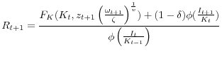
$\displaystyle R_{t+1}^{equity}=\frac{\frac{Y_{t+1}-\omega_{t+1}L_{t+1}}{K_{t}}+(1-\delta)p_{t+1}^{K}}{E_{t}[q_{t+1}\left(\frac{Y_{t+1}-\omega_{t+1}L_{t+1}}{K_{t}}+(1-\delta)p_{t+1}^{K}\right)]}.$

(5)

I define the aggregate return to investing as:

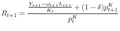
$\displaystyle R_{t+1}=\frac{\frac{Y_{t+1}-\omega_{t+1}L_{t+1}}{K_{t}}+(1-\delta)p_{t+1}^{K}}{p_{t}^{K}}$

(6)

Note that, due to idiosyncratic risk, the standard Q-theory result that $R_{t+1}=R_{t+1}^{equity}$ will not hold. Thus, (5) differs from the return on equity in production-based asset pricing papers such as Boldrin, Christiano and Fisher (2001), in which the price of a financial claim to aggregate firm assets is $p_{t}^{K}K_{t}$ and hence (5) is equal to (6). One contribution of the paper is to characterize how the investment wedge, $\frac{R_{t+1}}{R_{t+1}^{equity}}=E_{t}\left[q_{t+1}R_{t+1}\right]$ , and the equity premium, $\frac{E_{t}\left[R_{t+1}^{equity}\right]}{R_{t}^{rf}}$ , are related to idiosyncratic risk, parametrized by $P_{t}$ .

Remark 1. An alternative way to model financial contracting is to envision the creation of publicly traded, limited-liability equity claims on all future cash flows of a firm, when contracting between the managers and the equity holders is subject to the same moral hazard problem as in the sequential-trading "entrepreneurial" setup above. Suppose that, in period 0 , managers and investors meet and create a limited-liability publicly traded company. Each contributes wealth to create the company. The company is owned by the investors and signs a contract with the manager to provide a stream of consumption, given by $c_{t}^{i}$ , and to make a stream of investments in physical capital, given by $k_{t}^{e,i}$ , where $c_{t}^{i}$ and $k_{t}^{e,i}$ depend on the history of aggregate and idiosyncratic shocks. In this model, $c_{t}^{i}$ resembles managerial compensation. The managerial moral-hazard constraint is that the manager's lifetime utility $v_{t+1}^{i}$ must be greater than or equal to the outside option of absconding with $\left(1-\theta\right)$ share of the firm's assets, $a_{t+1}^{i}$ , and re-contracting with a new set of equity holders. This alternative model results in the same equilibrium policies, aggregate quantities and state price density as in the sequential-trading "entrepreneurial" setup above. Moreover, in general equilibrium, the return on the aggregate limited-liability equity claims is given by (5).

Remark 2. The return on equity is the return on an unlevered financial claim to aggregate firm assets. However, it is possible, as in Boldrin, Christiano and Fisher (2001), to study the return on a levered claim to aggregate firm assets:

$\displaystyle R_{t+1}^{levered}=R_{t+1}^{equity}+\lambda\left(R_{t+1}^{equity}-R_{t}^{rf}\right)$

where $\lambda$ measures leverage. The expected excess return on the levered claim is given by:

$\displaystyle \frac{E_{t}[R_{t+1}^{levered}]}{R_{t}^{rf}}=(1+\lambda)\frac{E_{t}[R_{t+1}^{equity}]}{R_{t}^{rf}}-\lambda$

2 Equilibrium characterization

2.1 Partial equilibrium

In the model, the firm's end-of-period assets and labor demand are linear in the manager's capital, due to constant returns to scale in technology and the ability to adjust labor demand according to the realization of the idiosyncratic shock:

$\displaystyle a_{t+1}^{i}=R_{t+1}p_{t}^{K}k_{t+1}^{i}$ and $\displaystyle l_{t+1}^{i}=l_{t+1}k_{t+1}^{i}$

where $l_{t+1}=\arg\max_{l}\left(F(1,z_{t+1}l)-\omega_{t+1}l\right)$ and $R_{t+1}=\frac{1}{p_{t}^{K}}\left(F(1,z_{t+1}l_{t+1})-\omega_{t+1}l_{t+1}+(1-\delta)p_{t+1}^{K}\right)$ .

Thus, the firm's problem can be written recursively as:

$\displaystyle V(w_{t}^{i};t)=\max_{k_{t}^{e,i},c_{t}^{i},\{w_{t+1}^{i}\}}U^{-1}\left[U(c_{t}^{i})+\beta U\left(\mathbb{CE}_{t}\left[V(w_{t+1}^{i};t+1)\right]\right)\right]$

(7)

subject to the budget constraint

$\displaystyle E_{t}\left[q_{t+1}w_{t+1}^{i}\right]\leq w_{t}^{i}-c_{t}^{i}+E_{t}\left[q_{t+1}R_{t+1}-1\right]p_{t}^{K}k_{t}^{e,i}$

and, for each $s_{t+1}^{i}$ , the limited-enforcement constraints

$\displaystyle w_{t+1}^{i}\geq(1-\theta)R_{t+1}p_{t}^{K}k_{t+1}^{i}$

(8)

Below, I guess and verify that

is linear in the manager's wealth. Thus, conditional on aggregate history $h^{t+1}$ and idiosyncratic history $h^{i,t}$ , manager

's wealth $w_{t+1}^{i}$ will equal some constant amount following every idiosyncratic shock $s_{t+1}^{i}$ below a threshold $s_{t}^{i*}$ , and for every state $s_{t+1}^{i}$ greater than this threshold, wealth will be determined by (8). That is, $w_{t+1}^{i}$ will be equal to the greater of a fixed amount or the minimum wealth level consistent with repayment. I denote the fixed amount by $n_{t+1}^{i}$ , so that

$\displaystyle w_{t+1}^{i}=\max\left\{ n_{t+1}^{i},(1-\theta)R_{t+1}p_{t}^{K}k_{t+1}^{i}\right\} .$

(9)

Using this intuition, firms' optimal decisions for given prices can be characterized.

Lemma 1 Given prices, optimal consumption $c_{t}^{i}$ , expected capital $k_{t}^{e,i}$ , and minimum payoff $n_{t+1}^{i}$ are linear in wealth $w_{t}^{i}$

$\displaystyle \frac{c_{t}^{i}}{w_{t}^{i}}$	$\displaystyle =$	$\displaystyle \tilde{c}_{t}$
$\displaystyle \frac{p_{t}^{K}k_{t}^{e,i}}{w_{t}^{i}}$	$\displaystyle =$	$\displaystyle (1-\tilde{c}_{t})\kappa_{t}$	(10)
$\displaystyle \frac{n_{t+1}^{i}}{w_{t}^{i}}$	$\displaystyle =$	$\displaystyle (1-\tilde{c}_{t})\eta_{t+1}$

and the consumption-wealth ratio $\tilde{c}_{t}$ satisfies:

$\displaystyle \frac{1}{\tilde{c}_{t}}=\left(\beta U\left(\rho_{t}\right)\right)^{\epsilon}+1$

(11)

where

$\displaystyle \rho_{t}=\mathbb{CE}_{t}\left[\tilde{c}_{t+1}^{\frac{1}{1-\epsilon}}\max\{\eta_{t+1},(1-\theta)s_{t+1}^{i}R_{t+1}\kappa_{t}\}\right]$

(12)

and

$\displaystyle \{\eta_{t+1},\kappa_{t}\}=\arg\max_{\{\eta\},\kappa}\mathbb{CE}_{t}\left[\tilde{c}_{t+1}^{\frac{1}{1-\epsilon}}\max\{\eta,(1-\theta)s_{t+1}^{i}R_{t+1}\kappa\}\right]$

(13)

subject to

$\displaystyle E_{t}\left[q_{t+1}\max\{\eta,(1-\theta)s_{t+1}^{i}R_{t+1}\kappa\}\right]\leq1+E_{t}\left[q_{t+1}R_{t+1}-1\right]\kappa$

(14)

Lemma 1 simplifies the manager's problem by transforming it into a canonical portfolio choice problem in which there is a single asset, with return

$\displaystyle R_{t+1}^{i}\equiv\max\{\eta_{t+1},(1-\theta)s_{t+1}^{i}R_{t+1}\kappa_{t}\}$

(15)

where $\eta_{t+1}$ and $\kappa_{t}$ are given by (13). The return on the single asset reflects the optimal mix of investments in physical capital and financial assets, given prices and the limited enforcement constraints.

Correspondingly, as in a canonical portfolio choice problem with Epstein Zin preferences, the lifetime utility function $V_{t}$ that solves the firm's problem is given by:

$\displaystyle V_{t}^{i}=\tilde{c}_{t}^{\frac{1}{1-\epsilon}}w_{t}^{i}$

Thus, $\rho_{t}$ is the period-

risk-adjusted return to saving, where return to saving is measured in units of the marginal lifetime utility of wealth, $\frac{dV_{t+1}^{i}}{dw_{t+1}^{i}}=\tilde{c}_{t+1}^{\frac{1}{1-\epsilon}}$ . That is,

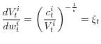
$\displaystyle \rho_{t}=\mathbb{CE}_{t}\left[\frac{dV_{t+1}^{i}}{dw_{t+1}^{i}}R_{t+1}^{i}\right]$

Managers' consumption choice is described by the Euler equation (11); a higher risk-adjusted return $\rho_{t}$ is consistent with lower consumption and greater investment if the elasticity of intertemporal substitution is greater than one.

To understand the manager's problem, consider manager 's pricing kernel $m_{t+1}^{i}$ , where

$\displaystyle m_{t+1}^{i}\equiv\frac{\partial v_{t}^{i}/\partial dc_{t+1}^{i}}{\partial v_{t}^{i}/\partial dc_{t}^{i}}=\beta\left(\frac{c_{t+1}^{i}}{c_{t}^{i}}\right)^{-\frac{1}{\epsilon}}\left(\frac{v_{t+1}^{i}}{\mathbb{CE}_{t}\left[v_{t+1}^{i}\right]}\right)^{\frac{1}{\epsilon}-\gamma}.$

(16)

(16) depends only on the assumption of Epstein Zin preferences. The Euler equation (11) can be stated as the familiar asset-pricing condition:

$\displaystyle E\left[m_{t+1}^{i}R_{t+1}^{i}\right]=1$

(17)

If there are no limited-enforcement constraints (that is, $\theta=1$ ), then equilibrium requires

$\displaystyle m_{t+1}^{i}=q_{t+1}$

and the model becomes a standard real-business cycle model. However, if $\theta<1$ , then

$\displaystyle m_{t+1}^{i}<q_{t+1}$

whenever the limited enforcement constraint (8) binds. That is, for $s_{t+1}^{i}>s_{t}^{i*}$ , the marginal lifetime utility from an additional unit of consumption is low, relative to the market price of consumption, but reducing wealth and consumption at state $s_{t+1}^{i}$ without violating the limited-enforcement constraint would require reducing $k_{t}^{e,i}$ , thus affecting consumption at other histories $h^{i,t+1}$ .

3 General equilibrium

3.1 Cross-sectional dynamics

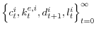
Define manager 's share of total managerial consumption by $\frac{c_{t}^{i}}{C_{t}^{M}}$ . The next result shows that risk sharing across managers is imperfect.

Lemma 2 The (gross) growth rate of manager 's consumption share in period is given by:

$\displaystyle g_{t+1}^{i}\equiv\frac{c_{t+1}^{i}/C_{t+1}^{M}}{c_{t}^{i}/C_{t}^{M}}=\max\{\psi_{t},(1-\theta)s_{t+1}^{i}\}$

(18)

where $\psi_{t}<1$ is the unique solution to

$\displaystyle E[\max\{\psi_{t},(1-\theta)s_{t+1}^{i}\}]=1.$

(19)

Lemma 2 implies that how idiosyncratic risk between period-

and period-

is shared depends only on the distribution of period-

idiosyncratic shocks and the extent of moral hazard, $1-\theta$ . This result follows from market clearing and the linearity of each manager's investment and consumption in her wealth.

Later, I will characterize how macroeconomic and financial variables respond to a mean-preserving spread in $g_{t+1}^{i}$ . A paper from the options literature, Rasmusen (2007), provides a definition of increased risk in $s_{t+1}^{i}$ that is useful here.

Definition The distribution $\widetilde{P}_{t}$ is pointwise riskier than $P_{t}$ if $s_{t+1}^{i}$ has the same mean under each distribution and if there exist

and

with $$ s^{min}<s'<s$ such that

$\displaystyle \tilde{p}_{t}$

$\displaystyle >$

$\displaystyle p_{t}$ $$\displaystyle \mbox{ for all \ensuremath{s_{t+1}^{i}\in[s^{min},s']\bigcup[s$

and $\tilde{p}_{t}\leq p_{t}$ otherwise.

An increase in pointwise riskiness shifts probability mass from each point in the middle of the support to points at each extreme of the support. As the next result shows, an increase in pointwise riskiness in $s_{t+1}^{i}$ is a sufficient condition for a mean-preserving spread in $g_{t+1}^{i}$ .²

Lemma 3 An increase in pointwise risk in $P_{t}$ leads to a mean-preserving spread in the growth rate of manager i's consumption share, $g_{t+1}^{i}$ , and a decrease in risk-sharing, $\psi_{t}$ .

According to Lemma 3, the growth rate of each manager's consumption share becomes riskier when idiosyncratic uncertainty increases. The deterioration of risk sharing has two components: the mechanical effect that $P_{t}$ is riskier; as well as an endogenous, general-equilibrium effect, in the form of a strict decrease in $\psi_{t}$ , the worst-case growth of manager

's consumption share. Intuitively, worst-case consumption-share growth decreases because, with greater uncertainty about idiosyncratic depreciation, managers seek to hedge all of their increased downside risk, but can only sell $\theta$ share of their increased upside risk.

3.2 Aggregate dynamics

Using the market-clearing condition $\kappa_{t}=1$ , one can write the idiosyncratic return to investment, defined in (15), as:

$\displaystyle R_{t+1}^{i}=g_{t+1}^{i}R_{t+1}$

(20)

The term $g_{t+1}^{i}$ reflects idiosyncratic risk, given by (18). The term $R_{t+1}$ is the aggregate return to investment, given by (6).

Profit maximization of consumption-goods firms and capital-goods firms, together with labor market clearing, implies

$\displaystyle R_{t+1}=\frac{F_{K}(K_{t},z_{t+1}\left(\frac{\omega_{t+1}}{\zeta}\right)^{\frac{1}{v}})+(1-\delta)\phi(\frac{I_{t+1}}{K_{t}})}{\phi\left(\frac{I_{t}}{K_{t-1}}\right)}$

where $\omega_{t+1}$ is the unique solution to

$\displaystyle \omega_{t+1}=F_{L}(K_{t},z_{t+1}\left(\frac{\omega_{t+1}}{\zeta}\right)^{\frac{1}{v}})z_{t+1}.$

(21)

These results permit further characterization of the dynamics of aggregate capital and consumption.

Proposition 4 The path for aggregate capital, $K_{t},$ aggregate consumption, $C_{t}$ , and the price of physical capital, $p_{t}^{K}$ , are the same as in a model without investment risk ( $\theta=1$ ), but with a different discount factor $\bar{\beta}_{t}$ that follows a stochastic process given by:

$\displaystyle \bar{\beta}_{t}=\beta U\left(\mathbb{CE}_{t}[g_{t+1}^{i}]\right)$

(22)

where $g_{t+1}^{i}$ is the growth rate of manager i's share of aggregate managerial consumption, given by (18). A mean-preserving spread in $g_{t+1}^{i}$ is associated with a decrease in the equivalent discount factor $\bar{\beta}_{t}$ if and only if $\epsilon>1$ .

Proof. Combining (11) and (12), we obtain the Euler equation:

$\displaystyle \tilde{c}_{t}=\frac{1}{\left(\beta U\left(\mathbb{CE}_{t}\left(\tilde{c}_{t+1}^{\frac{1}{1-\epsilon}}R_{t+1}^{i}\right)\right)\right)^{\epsilon}+1}.$

where $R_{t+1}^{i}$ is given by (20). Because the growth rate of the idiosyncratic consumption share, $g_{t+1}^{i}$ , is independent of $h_{t+1}$ , we can re-write this as:

$\displaystyle \tilde{c}_{t}=\frac{1}{\left(\beta U\left(\mathbb{CE}_{t}\left(g_{t+1}^{i}\right)\right)U\left(\mathbb{CE}_{t}\left(\tilde{c}_{t+1}^{\frac{1}{1-\epsilon}}R_{t+1}\right)\right)\right)^{\epsilon}+1}$

That is, conditional on the aggregate return to investing $R_{t+1}$ , the consumption share of wealth $\tilde{c}_{t}$ will be the same as in a model without investment risk but with a discount factor given by (22). Therefore, the equilibrium path for aggregate capital and consumption will be the same in both models and hence the path for the aggregate return to investing will be the same as well. $\qedsymbol$

If there is no aggregate uncertainty about idiosyncratic risk (e.g., if $P_{t}=P$ for all

), then aggregate quantities are the same as in a model without investment risk ( $\theta=1$ ), but with an adjusted discount factor. The direction of adjustment depends on the EIS: if managers are willing to substitute across time $(\epsilon>1)$ , a mean-preserving spread in $g_{t+1}^{i}$ makes the managers more reluctant to invest. The intuition is that an increase in idiosyncratic risk leads to a decrease in the risk-adjusted return to saving; in response, managers will consume more and save less if they are willing to substitute across time.

Similarly, if there is aggregate uncertainty about idiosyncratic risk (e.g., if $P_{t}$ follows a stochastic process), then aggregate quantities are the same as in a model without investment risk ( $\theta=1$ ), but with time-preference shocks.³

3.3 Asset pricing and the investment wedge

It is not the case that shocks to idiosyncratic uncertainty are isomorphic to time-preference shocks. In particular, the prices of financial assets are different than in the model without investment risk, but with time-preference shocks given by (22), even though the paths for aggregate quantities and the price of physical capital are the same.

One way to see this is to examine how the equilibrium state-price density $q_{t+1}$ is related to the state-price density in a model without investment risk, but with time-preference shocks.

Lemma 5 At time , the state-price density $q_{t+1}$ is the same, up to a pre-determined scalar, as in a model without investment risk ( $\theta=1$ ) but with stochastic discount factor $\bar{\beta}_{t}$ given by (22). That is, if $q_{t+1}^{\beta}$ is the state-price density in the model without investment risk and with time-preference shocks given by (22), then

$\displaystyle \frac{q_{t+1}}{q_{t+1}^{\beta}}=\frac{\mathbb{CE}_{t}[\frac{g_{t+1}^{i}}{\psi_{t}}]^{\gamma}}{\mathbb{CE}_{t}[g_{t+1}^{i}]}>1.$

(23)

Proof. For any idiosyncratic history $h^{i,t+1}$ for which the limited-enforcement constraint (8) is not binding, we have $q_{t+1}=m_{t+1}^{i}$ . Hence, substituting into (16), we have

$\displaystyle q_{t+1}=\beta\left(\frac{\tilde{c}_{t+1}}{\tilde{c}_{t}}\psi_{t}R_{t+1}(1-\tilde{c}_{t})\right)^{-\frac{1}{\epsilon}}\left(\frac{\tilde{c}_{t+1}^{\frac{1}{1-\epsilon}}\psi_{t}R_{t+1}}{\mathbb{CE}_{t}\left[\tilde{c}_{t+1}^{\frac{1}{1-\epsilon}}g_{t+1}^{i}R_{t+1}\right]}\right)^{\frac{1}{\epsilon}-\gamma}$

Because the growth rate of the idiosyncratic consumption share, $g_{t+1}^{i}$ , is independent of $h_{t+1}$ , we can write

$\displaystyle q_{t+1}=\beta\left(\frac{\tilde{c}_{t+1}}{\tilde{c}_{t}}\psi_{t}R_{t+1}(1-\tilde{c}_{t})\right)^{-\frac{1}{\epsilon}}\left(\frac{\tilde{c}_{t+1}^{\frac{1}{1-\epsilon}}\psi_{t}R_{t+1}}{\mathbb{CE}_{t}\left[\tilde{c}_{t+1}^{\frac{1}{1-\epsilon}}R_{t+1}\right]\mathbb{CE}_{t}\left(g_{t+1}^{i}\right)}\right)^{\frac{1}{\epsilon}-\gamma}$

which, together with (22), implies (23). Finally, (19) and Lemma 2 imply $\frac{q_{t+1}}{q_{t+1}^{\beta}}>1$ . $\qedsymbol$

This result has immediate implications for the investment wedge, the risk-free rate and the equity premium.

3.3.1 Investment wedge

In a model without idiosyncratic investment risk ( $\theta=1$ ), the return on investment, (6), would equal the return on equity, (5). Correspondingly, we would have:

$\displaystyle E_{t}[q_{t+1}R_{t+1}]=1.$

(24)

This no-arbitrage condition is the standard Q-theory result that financial-market prices $q_{t+1}$ can price the return to investing in physical capital.

However, with idiosyncratic investment risk, (24) does not hold. Because investing in physical capital involves idiosyncratic risk, managers need to compensated to bear these risks. This will take the form of an investment wedge.

Proposition 6 The investment wedge, $\frac{R_{t+1}}{R_{t+1}^{equity}}=E_{t}[q_{t+1}R_{t+1}]$ , is greater than one.

Proposition 6 is a corollary of Lemma 5. To see this, substitute from (23) to write the investment wedge as:

$\displaystyle E[q_{t+1}R_{t+1}]$

$\displaystyle =$

$\displaystyle \frac{q_{t+1}}{q_{t+1}^{\beta}}E_{t}[q_{t+1}^{\beta}R_{t+1}]=\frac{q_{t+1}}{q_{t+1}^{\beta}}$

(25)

From Proposition 4, we have that the equilibrium path for $R_{t+1}$ is the same as in the model without investment-risk, but with time-preference shocks given by (22). Note that in the model without investment risk, the state-price density that prices financial assets $q_{t+1}^{\beta}$ will price the return to investing in physical capital, $R_{t+1}$ ; that is, $E_{t}[q_{t+1}^{\beta}R_{t+1}]=1$ . The result then follows from Lemma 5.

3.3.2 The equity premium and the risk-free rate

Additional corollaries of Lemma 5 concern the risk-free rate and the equity premium:

Proposition 7 The equity premium, $\frac{E_{t}\left[R_{t+1}^{equity}\right]}{R_{t}^{rf}}$ , is the same as in the model without investment risk, but with stochastic discount factor $\bar{\beta}_{t}$ given by (22).

Proof. From (5) and (6), the equity premium is given by:

$\displaystyle \frac{E_{t}\left[R_{t+1}^{equity}\right]}{R_{t}^{rf}}$	$\displaystyle =$	$\displaystyle \frac{E_{t}\left[R_{t+1}\right]}{E_{t}\left[q_{t+1}R_{t+1}\right]}E_{t}[q_{t+1}]$
	$\displaystyle =$	$\displaystyle \frac{E_{t}\left[R_{t+1}\right]}{E_{t}\left[q_{t+1}^{\beta}R_{t+1}\right]}E_{t}[q_{t+1}^{\beta}]$	(26)

where the second equality follows from (23). (26) is the equity premium in the model without investment risk, but with stochastic discount factor $\bar{\beta}_{t}$ . $\qedsymbol$

Proposition 8 The risk-free rate, $R_{t}^{rf}=E_{t}[q_{t+1}]^{-1}$ , will be lower than in the model without investment risk, but with stochastic discount factor $\bar{\beta}_{t}$ given by (22).

Proof. Substitute from (23) to write the risk-free rate as:

$\displaystyle R_{t}^{rf}=E_{t}\left[q_{t+1}^{\beta}\right]^{-1}\frac{q_{t+1}^{\beta}}{q_{t+1}}$

(27)

In the model without investment risk, but with time-preference shocks, the risk-free rate is given by $E_{t}\left[q_{t+1}^{\beta}\right]^{-1}$ . And, from Lemma 5, $q_{t+1}>q_{t+1}^{\beta}$ . $\qedsymbol$

Thus, although aggregate quantities and the equity premium are same as in a model without investment risk, but with time-preference shocks given by (22), the risk-free rate is lower.

3.3.3 Effects of an increase in idiosyncratic uncertainty

Next, I will characterize how the investment wedge and the state-price density change in response to an increase in idiosyncratic uncertainty.

Proposition 9 There exists a $\overline{\gamma}>1$ such that, if $\gamma<\overline{\gamma}$ , an increase in pointwise risk in $P_{t}$ leads to a strict increase in the investment wedge $\frac{R_{t+1}}{R_{t+1}^{equity}}=\frac{q_{t+1}}{q_{t+1}^{\beta}}$ ; and a strict decrease in the ratio of the risk-free rate to the risk-free rate that would obtain in the model without investment risk, but with stochastic discount factor $\bar{\beta}_{t}$ given by (22).

Proposition 9 highlights the different forces affecting asset pricing in a general equilibrium environment with idiosyncratic risk. As is well known from Hadar and Seo (1990) and Gollier (1995), in a standard partial-equilibrium portfolio problem with one safe asset and one risky asset, a mean-preserving spread in the return on the risky asset does not, in general, imply that a risk-averse agent will reduce her allocation to the risky asset. Instead, with constant relative risk aversion, Hadar and Seo (1990) show that a mean-preserving spread leads to a decrease in the allocation to that asset if $\gamma<1$ . Correspondingly, in my model, if $\gamma>1$ , it is possible to construct a mean-preserving spread in $s_{t+1}^{i}$ such that the investment wedge decreases. In particular, any mean-preserving spread in $s_{t+1}^{i}$ that leaves the density unchanged for all $s_{t+1}^{i}<s_{t}^{*}$ will result in a strict decrease in the investment wedge. However, with an increase in pointwise risk in $s_{t+1}^{i}$ , there is always an endogenous increase in "downside risk," in the form of a strict decrease in $\psi_{t}$ . This guarantees that if relative risk aversion is not too large, an increase in pointwise risk in $s_{t+1}^{i}$ will lead to an increase in the investment wedge.⁴

It also possible to define a stricter notion of an increase in risk such that the investment wedge increases with risk, for every $\gamma$ . In particular, recall that a pointwise increase in risk transfers probability mass from the middle of the distribution, with $$ s_{t+1}^{i}\in(s',s$ to the lower and upper parts of the distribution, with $$ s_{t+1}^{i}\in[s^{min},s']\bigcup[s$ . Any pointwise increase in risk with $s^{\eta} < s_{t}^{*}$ leads to a strict increase in the investment wedge.⁵

3.4 Deterministic steady state

If there is no aggregate uncertainty, we can characterize the steady state of the economy:

Proposition 10 Suppose that

$\displaystyle \epsilon>\underline{\epsilon}\equiv\left[1+\frac{\log\beta}{\log\left(\mathbb{CE}_{t}[g_{t+1}^{i}]\right)}\right]^{-1}.$

(28)

Then there exist unique steady-state values $K^{*},C^{*},L^{*},I^{*},Y^{*}.$ A mean-preserving spread in $g_{t+1}^{i}$ is associated with a decrease in $K^{*},C^{*},L^{*},I^{*},Y^{*}$ if and only if $\epsilon>1$ .

Proposition 10 follows from the result that aggregate quantities are the same as in an economy without investment risk, but with a different discount factor given by (22). If $\epsilon>\underline{\epsilon}$ , the equivalent discount factor is less than one and a unique steady state exists. Moreover, steady-state aggregate capital, consumption and employment decrease to a lower steady state following an increase in idiosyncratic risk if and only if $\epsilon>1$ . To see this, note that aggregate quantities respond to an increase in idiosyncratic risk as if managers were more impatient, if and only if $\epsilon>1$ .

We can also further characterize the risk-free rate. If $\epsilon>\underline{\epsilon}$ , there is a unique steady-state value for the risk-free rate, given by:

$\displaystyle R^{rf*}=\frac{1}{\beta}\psi_{t}^{\gamma}\mathbb{CE}_{t}[g_{t+1}^{i}]^{\frac{1}{\epsilon}-\gamma}<\frac{1}{\beta}$

(29)

Proposition 8 implies the inequality in (29). The analogous result to Proposition 9 is that if relative risk aversion $\gamma$ is not too high, an increase in pointwise risk in $P_{t}$ leads to a strict decrease in the risk-free rate. However, whereas the threshold in Proposition 9 was $\overline{\gamma}>1$ , here it is $\overline{\gamma}>\frac{1}{\epsilon}$ . Similarly, any pointwise increase in risk with

leads to a strict decrease in the risk-free rate.

4 Quantitative implications of idiosyncratic investment risk

The calibration approach here is to characterize the financial and macroeconomic response to a shock to idiosyncratic uncertainty, while making as few as possible parametric assumptions. Specifically, for several $P_{t}\in\mathbf{P}$ , I calculate the distribution of idiosyncratic consumption growth, $g_{t+1}^{i}$ , and the investment wedge, $\frac{R_{t+1}}{R_{t+1}^{equity}}$ . I also calculate, for several $P_{t}\in\mathbf{P}$ , the discount factor $\bar{\beta}_{t}$ such that aggregate quantities and the equity premium in the model are the same as in a model without idiosyncratic investment risk, but with discount factor $\bar{\beta}_{t}$ . In doing so, I do not need additional assumptions about the technologies for producing consumption and capital goods. Also, I will not have to specify the Markov process for the technology shock $z_{t}$ and the idiosyncratic risk shock $P_{t}$ . That is, the results presented are such that, for any given Markov process for $P_{t}\in\mathbf{P}$ , one can calculate the Markov process for $\bar{\beta}_{t}$ . Although this approach offers only a partial characterization of the dynamics of the economy, the results will be consistent with, for example: an AR(1) process for the (log) standard deviation of idiosyncratic shocks (as in Gilchrist, Sim and Zakrajek (2013)); or an AR(1) process for the $\mathit{growth}$ rate of the standard deviation of idiosyncratic shocks (which would give rise to "quantity-equivalent" time-preference shocks similar to those in Albuquerque, Eichenbaum and Rebelo (2012)). Also, previous theoretical results will be informative about how the calibration results would vary with different parametric assumptions: for example, the investment wedge does not depend on the EIS, and the "quantity-equivalent" discount factor is decreasing in the EIS.

In addition, I calculate the marginal product of capital and the risk-free rate that would prevail in the steady state of the model when there is no aggregate uncertainty.

4.1 Parameter choice

I assume that $s_{t+1}^{i}$ follows a Pareto distribution with standard deviation $\sigma_{t}\in(0,\infty)$ . As before, I assume $E_{t}[s_{t+1}^{i}]=1$ . Thus, the tail parameter $\alpha_{t}$ satisfies

$\displaystyle \alpha_{t}=1+\sqrt{1+\sigma_{t}^{-2}}>2$

and the cumulative distribution function $P_{t}$ is given by

$\displaystyle P_{t}(s_{t+1}^{i})=1-\left(1-\alpha_{t}^{-1}\right)^{\alpha_{t}}\left(s_{t+1}^{i}\right)^{-\alpha_{t}}$

for any $s_{t+1}^{i}\geq1-\alpha_{t}^{-1}$ . Below, I repeat the analysis under the alternative assumption that $s_{t+1}^{i}$ follows a log-normal distribution.

In the literature on idiosyncratic investment risk, Panousi (2012) uses a constant value of $\sigma=0.3$ , while Roussanov (2010) sets $\sigma=0.45$ . Using panel data on private-business income, DeBacker et al. (2012) also suggest $\sigma=0.45$ . One can also use idiosyncratic stock-market returns to calibrate $\sigma_{t}$ , consistent with the public-company implementation of financial markets discussed in Section 2. Goyal and Santa-Clara (2003) find that the average volatility of individual stock returns is 16 percent per month, suggestive of annual volatility of individual stock returns between 50 and 60 percent. Thus, below I consider $\sigma_{t}\in[0.15,0.6]$ . The corresponding range for the Pareto tail parameter is $\alpha_{t}\in\left[2.9,7.7\right].$

To calibrate the risk-sharing technology (parametrized by $\theta$ in this model), the literature on idiosyncratic investment risk typically looks to data on the volatility of idiosyncratic consumption growth. Of course, disaggregated consumption data is subject to a variety of limitations: there is significant measurement error; households in the Consumer Expenditure Survey (CEX) are followed for only a short period of time; and idiosyncratic consumption may be driven by deterministic factors such as age and aggregate consumption. To deal with these issues, Blundell, Pistaferri and Preston (2008) impute consumption using the Panel Study of Income Dynamics and the CEX, and regress imputed log annual consumption on year and year-of-birth dummies and a range of family characteristics. The first difference of these residuals corresponds, in my model, to the log of the consumption-share growth rate, $\log(g_{t+1}^{i})$ . Using the results in Blundell, Pistaferri and Preston (2008), a reasonable estimate of the cross-sectional standard deviation of this first difference is 13 percent per annum.⁶ Blundell, Pistaferri and Preston (2008) study consumption dynamics for the entire population. In this paper, the focus is on investors and managers. Jacobs and Wang (2004) estimate the standard deviation of idiosyncratic consumption growth across all households and also limiting the sample only to asset holders. Averaging across time, they find that the mean standard deviation across all households is roughly similar to the mean standard deviation across asset holders. However, controlling for age and education, Jacobs and Wang find that the standard deviation of idiosyncratic consumption growth across asset holders is about 50 percent larger than the standard deviation across all households.

A number of calibration exercises make explicit or implicit choices about the volatility of the idiosyncratic consumption share. De Santis (2007) assumes that the cross-sectional standard deviation of $\log(g_{t+1}^{i})$ has a mean of 10 percent. In Panousi (2012), the standard deviation of idiosyncratic consumption growth, in the steady state, is 7 percent. As a benchmark, I choose a value of $\theta=0.3$ , which results in a cross-sectional standard deviation of the log idiosyncratic consumption share growth rate equal to 8 percent if $\sigma_{t}=0.3$ .

For the elasticity of intertemporal substitution, I choose $\epsilon=2$ . Gourio (2012) chooses the same value. An EIS greater than one is required for an increase in idiosyncratic uncertainty to generate an economic contraction. I also consider how a lower EIS effects the results. I set the discount factor $\beta$ equal to 0.95 and the coefficient of relative risk aversion $\gamma$ equal to 4.

4.2 Effects of idiosyncratic uncertainty on financial and macroeconomic variables

Table 1 shows how different levels of idiosyncratic uncertainty affect risk sharing, macroeconomic dynamics and risk premia. The first column corresponds to the benchmark case, with $\sigma_{t}=0.3$ . The second and third columns correspond to a 50 percent and a 100 percent increase in the standard deviation of idiosyncratic shocks, as in Bloom (2009). The final column represents a 50 percent decrease in the standard deviation of idiosyncratic shocks.

Relative to the benchmark case, a 50 percent increase in $\sigma_{t}$ leads to a roughly proportional increase in the volatility of idiosyncratic consumption. In the benchmark case, the lower bound of idiosyncratic consumption-share growth, $\psi_{t}$ , is fairly high: following the worst possible shock, which corresponds to a decrease in capital of about 20 percent, a manager's consumption share falls only 2 percent.⁷ With a 50 percent increase in $\sigma_{t}$ , a manager's consumption share falls twice as much (that is, about 4 percent) following a bad shock.

The macroeconomic and financial effects of idiosyncratic risk are summarized in the next rows. With a 50 percent increase in $\sigma_{t},$ the response of aggregate quantities and the equity premium are the same as in a model without investment risk, but with a discount-factor shock of approximately 70 basis points. That is, aggregate quantities and the equity premium respond as if there were no investment risk, but the discount factor decreased from 0.945 to 0.938. At the same time, the investment wedge - the spread between the return on a firm's physical capital and the return on financial claims on the firm - increases from 5 percentage points to 10 percentage points. That is, in the benchmark case, firms invest as if their cost of capital were 5 percentage points higher than it actually is; with a 50 percent increase in idiosyncratic uncertainty, that wedge increases to 10 percentage points. Equivalently, the risk-free rate following the uncertainty shock will be about 5 percentage points lower than in a model without investment risk, but with a discount-factor shock that generates the same response for aggregate quantities.

The final row shows the steady-state risk-free rate that would obtain if there were no aggregate uncertainty. In the benchmark case, the risk-free rate would be about 1 percentage point per year. With a 50 percent increase in $\sigma_{t}$ , the risk-free rate would be -3 percentage points per year. These results show that, due to imperfect risk sharing, shocks to idiosyncratic uncertainty of the size contemplated in Bloom (2009). can lead to very large shocks to the real risk-free rate, of similar magnitude to the exogenous "shock to the natural rate of interest" studied in Eggertsson and Woodford (2003) and Christiano, Eichenbaum and Rebelo (2011).

If the EIS were different, the distribution of idiosyncratic consumption-share growth, $g_{t+1}^{i}$ , and the investment wedge would not change. Thus, the only variables reported in Table 1 that would change are the "quantity-equivalent" discount factor, $\bar{\beta}_{t}$ , and the steady-state risk-free rate that would obtain if there were no aggregate uncertainty. From (22) and (27), one observes that, all else equal, $\bar{\beta}_{t}$ is decreasing in the EIS and that $R^{rf*}$ is increasing in the EIS. As shown in Table 2, the size of the quantity-equivalent discount-factor shock corresponding to a 50 percent increase in idiosyncratic uncertainty would be somewhat smaller if the EIS were 1.5, at 50 basis points, rather than 70 basis points. The steady-state risk-free rate at the baseline level of idiosyncratic uncertainty would be 20 basis points lower, and a 50 percent increase in idiosyncratic risk would result in a slightly larger drop in the steady-state risk-free rate.

Unlike a change in the EIS, a change in relative risk aversion would affect the investment wedge, as shown in Table 3. If relative risk aversion were halved, the investment wedge would be 3 percentage points at the baseline level of idiosyncratic uncertainty, rather 5 percentage points. Moreover, a 50 percent increase in idiosyncratic uncertainty would lead to an investment wedge of 7 percentage points, rather than 10 percentage points. Similarly, the effects of idiosyncratic uncertainty on the "quantity-equivalent" discount factor and the steady-state risk-free rate would also be somewhat smaller if relative risk aversion were halved.

Finally, Table 4 shows how the results would be affected by assuming that $P_{t}$ is log-normal, rather than Pareto.⁸ At the baseline level of idiosyncratic uncertainty, assuming that $P_{t}$ is log-normal implies that idiosyncratic consumption volatility is somewhat lower, and the lower-bound on consumption-share growth is a bit higher. Correspondingly, at the baseline level of idiosyncratic uncertainty, if $P_{t}$ is log-normal, the quantity-equivalent discount factor and the steady-state risk-free rate are slightly higher, and the investment wedge is slightly lower.

However, at higher levels of idiosyncratic uncertainty, the effects of idiosyncratic uncertainty are much larger if $P_{t}$ is log-normal than if $P_{t}$ is Pareto. Following a shift from $\sigma_{t}=0.3$ to $\sigma_{t}=0.45$ , the volatility of idiosyncratic consumption-share growth increases 7 percentage points, and the lower-bound on the consumption-share growth rate falls 3 percentage points. Correspondingly, the quantity-equivalent discount-factor shock and the increase in the investment wedge are larger in magnitude than if $P_{t}$ is Pareto.

5 Conclusion

In this paper, I have argued that shocks to uncertainty about idiosyncratic return on investment can explain the aftermath of financial crisis - elevated risk premia, a sharp and persistent decrease in investment, and a decrease in the risk-free rate. More specifically, aggregate quantities and the equity premium respond to an increase in idiosyncratic uncertainty as if there were no idiosyncratic investment risk and instead managers experienced an "impatience" time-preference shock. However, unlike an impatience shock, an increase in idiosyncratic uncertainty leads to a decrease in the risk-free rate.

Thus, a shock to idiosyncratic uncertainty is similar to the "risk premium" shock that Smets and Wouters (2007) , Gali, Smets and Wouters (2011) and Gali, Smets and Wouters (2012) find is important for explaining short-run movements in output, employment and interest rates, as well as the depth of and slow recovery from the Great Recession. In these papers, the "risk premium" shock makes it unattractive to hold physical capital. In order for the risk-free rate to fall meaningfully following such a shock, one needs the supply of financial assets to be somewhat inelastic. In Smets and Wouters (2003), this is the case because the only financial asset is a government bond, and government spending is exogenous. In my paper, following a shock to uncertainty about idiosyncratic rate of return, the supply of financial assets is somewhat inelastic because the way to create financial assets is by deploying more physical capital. Thus, as each manager seeks to shift from investing in her own physical capital to investing in diversified claims on other managers' physical capital, the other managers are trying to do the same.

References

Albuquerque, Rui, Martin S Eichenbaum, and Sergio Rebelo. 2012. Valuation risk and asset pricing. National Bureau of Economic Research.

Angeletos, George-Marios. 2007. Uninsured idiosyncratic investment risk and aggregate saving. Review of Economic Dynamics, 10(1): 1-30.

Angeletos, George-Marios, and Vasia Panousi. 2009.Revisiting the supply side effects of government spending. Journal of Monetary Economics, 56(2): 137-153.

Angeletos, George-Marios, and Vasia Panousi. 2011. Financial integration, entrepreneurial risk and global dynamics. Journal of Economic Theory, 146(3): 863-896.

Bloom, Nicholas. 2009. The impact of uncertainty shocks. Econometrica, 77(3): 623-685.

Blundell, Richard, Luigi Pistaferri, and Ian Preston. 2008. Consumption inequality and partial insurance. American Economic Review, 98(5): 1887-1921.

Boldrin, Michele, Lawrence J Christiano, and Jonas DM Fisher. 2001. Habit persistence, asset returns, and the business cycle. American Economic Review, 91(1): 149-166.

Buera, Francisco J, and Benjamin Moll. 2012. Aggregate implications of a credit crunch. National Bureau of Economic Research.

Christiano, Lawrence, Martin Eichenbaum, and Sergio Rebelo. 2011. When Is the Government Spending Multiplier Large? Journal of Political Economy, 119(1): 78-121.

DeBacker, Jason, Bradley Heim, Vasia Panousi, Shanthi Ramnath, and Ivan Vidangos. 2012. The properties of income risk in privately held businesses. Mimeo, Federal Reserve Board.

De Santis, Massimiliano. 2007. Individual consumption risk and the welfare cost of business cycles. American Economic Review, 97(4).

Eggertsson, Gauti B, and Michael Woodford. 2003. Zero bound on interest rates and optimal monetary policy. Brookings Papers on Economic Activity , 2003(1): 139-233.

Gali, Jordi, Frank Smets, and Rafael Wouters. 2011. Unemployment in an estimated new keynesian model. National Bureau of Economic Research.

Gali, Jordi, Frank Smets, and Rafael Wouters. 2012. Slow recoveries: a structural interpretation. Journal of Money, Credit and Banking, 44(2): 9-30.

Gilchrist, Simon, Jae W. Sim, and Egon Zakrajek. 2013. Uncertainty, Financial Frictions, and Irreversible Investment. Mimeo, Boston University.

Gollier, Christian. 1995. The comparative statics of changes in risk revisited. Journal of Economic Theory, 66(2): 522-535.

Gourio, Francois. 2012. Disaster Risk and Business Cycles. American Economic Review , 102(6): 2734-2766.

Gourio, Francois. 2013. Credit Risk and Disaster Risk. American Economic Journal: Macroeconomics, 5(3): 1-34.

Goyal, Amit, and Pedro Santa-Clara. 2003. Idiosyncratic risk matters! The Journal of Finance, 58(3): 975-1008.

Hadar, Josef, and Tae Kun Seo. 1990. The effects of shifts in a return distribution on optimal portfolios. International Economic Review, 31(3): 721-736.

Hall, Robert E. 2013. High Discounts and High Unemployment. Mimeo, Stanford University.

Jacobs, Kris, and Kevin Q Wang. 2004. Idiosyncratic consumption risk and the cross section of asset returns. The Journal of Finance, 59(5): 2211-2252.

Panousi, Vasia. 2012. Capital taxation with entrepreneurial risk. Mimeo, Federal Reserve Board.

Panousi, Vasia, and Dimitris Papanikolaou. 2012. Investment, idiosyncratic risk, and ownership. The Journal of Finance, 67(3): 1113-1148.

Rasmusen, Eric. 2007. When Does Extra Risk Strictly Increase an Option's Value? Review of Financial Studies, 20(5): 1647-1667.

Roussanov, Nikolai. 2010. Diversification and its discontents: Idiosyncratic and entrepreneurial risk in the quest for social status. The Journal of Finance, 65(5): 1755-1788.

Smets, Frank, and Raf Wouters. 2003. An estimated dynamic stochastic general equilibrium model of the euro area. Journal of the European Economic Association, 1(5): 1123-1175.

Smets, Frank, and Raf Wouters. 2007. Shocks and frictions in US business cycles: A Bayesian DSGE approach. American Economic Review, 97(3): 586-606.

Appendix: Proofs omitted from the text

Proof of Lemma 1

Define

$\displaystyle B(x_{t}^{i})=\max_{k_{t}^{e,i},\{w_{,t+1}^{i}\}}\mathbb{CE}_{t}\left[V(w_{t+1}^{i};t+1)\right]$

(30)

subject to

$\displaystyle E_{t}\left[q_{t+1}w_{t+1}^{i}\right]\leq x_{t}^{i}+E_{t}\left[q_{t+1}R_{t+1}-1\right]p_{t}^{K}k_{t}^{e,i}$

and (8). Using (30), we can re-write (7) as

$\displaystyle V(w_{t}^{i};t)=\max_{x_{t}^{i}}U^{-1}\left[U(w_{t}^{i}-x_{t}^{i})+\beta U\left(B(x_{t}^{i};t\right)\right]$

(31)

Conjecture the following solution:

$\displaystyle V(w_{t}^{i};t)$	$\displaystyle =$	$\displaystyle \xi_{t}w_{t}^{i}$	(32)
$\displaystyle \frac{c_{t}^{i}}{w_{t}^{i}}$	$\displaystyle =$	$\displaystyle \tilde{c}_{t}$	(33)
$\displaystyle \frac{p_{t}^{K}k_{t}^{e,i}}{w_{t}^{i}}$	$\displaystyle =$	$\displaystyle (1-\tilde{c}_{t})\kappa_{t}$
$\displaystyle \frac{n_{t+1}^{i}}{w_{t}^{i}}$	$\displaystyle =$	$\displaystyle (1-\tilde{c}_{t})\eta_{t+1}$

where $\xi_{t}$ is an endogenous random variable.

Substituting from (9) and (32) into (30), one obtains:

$\displaystyle B(x_{t}^{i})=\max_{k_{t}^{e,i},\{w_{,t+1}^{i}\}}\mathbb{CE}_{t}\left[\xi_{t+1}\max\left\{ n_{t+1}^{i},(1-\theta)R_{t+1}s_{t+1}^{i}p_{t}^{K}k_{t}^{e,i}\right\} \right]$

(34)

subject to

$\displaystyle E_{t}\left[q_{t+1}\max\left\{ n_{t+1}^{i},(1-\theta)R_{t+1}s_{t+1}^{i}p_{t}^{K}k_{t}^{e,i}\right\} \right]\leq x_{t}^{i}+E_{t}\left[q_{t+1}R_{t+1}-1\right]p_{t}^{K}k_{t}^{e,i}$

(35)

Dividing the first-order condition with respect to $k_{t}^{e,i}$ by the first-order condition with respect to $n_{t+1}^{i}$ , one obtains:

$\displaystyle \frac{n_{t+1}^{i}}{p_{t}^{K}k_{t}^{e,i}}=\left(\left(\frac{(1-\theta)E_{t}\left[q_{t+1}R_{t+1}s_{t+1}^{i}\mathbf{1}\{s_{t+1}^{i}>s_{t+1}^{i*}\}\right]-E_{t}\left[q_{t+1}R_{t+1}-1\right]}{(1-\theta)^{1-\gamma}E_{t}\left[\left(\xi_{t+1}R_{t+1}s_{t+1}^{i}\right)^{1-\gamma}\mathbf{1}\{s_{t+1}^{i}>s_{t+1}^{i*}\}\right]}\right)\frac{\xi_{t+1}^{1-\gamma}}{q_{t+1}}\right)^{\frac{1}{\gamma}}$

where $s_{t+1}^{i*}$ is defined by $n_{t+1}^{i}=(1-\theta)R_{t+1}s_{t+1}^{i*}p_{t}^{K}k_{t}^{e,i}$ . This, together with the linearity of (35), implies that the solutions $n_{t}^{i}$ and $k_{t}^{i}$ to (34)-(35) are linear in $x_{t}^{i}$ and that $B(x_{t}^{i};t)$ is linear in $x_{t}^{i}$ . Then, from (31), one obtains that $x_{t}^{i}$ and $c_{t}^{i}$ are linear in $w_{t}^{i}$ , consistent with (33).

Next, using the envelope condition of (31), one obtains:

$\displaystyle \frac{dV_{t}^{i}}{dw_{t}^{i}}=\left(\frac{c_{t}^{i}}{V_{t}^{i}}\right)^{-\frac{1}{\epsilon}}=\xi_{t}$

Substituting from (32) and (33), we have

$\displaystyle \xi_{t}=\tilde{c}_{t}^{\frac{1}{1-\epsilon}}$

and thus

$\displaystyle B(x_{t}^{i})=\rho_{t}x_{t}^{i}.$

(36)

Substituting (36) into (31) and taking the first-order condition with respect to $x_{t}^{i}$ , one obtains (11). $\diamondsuit$

Proof of Lemma 2

From Lemma 1, each manager's investment and consumption decisions are linear in her wealth. Thus, we have that $g_{t+1}^{i}=\frac{R_{t+1}^{i}}{R_{t+1}}.$ Market clearing requires that $\kappa_{t}=1$ : all consumption goods that are not consumed are used as inputs to create capital goods. Financial market clearing implies that, for each $h^{t+1}$ ,

$\displaystyle \int_{s^{min}}^{s^{max}}R_{t+1}^{i}dP_{t}(s_{t+1}^{i})=R_{t+1}.$

Dividing both sides by $R_{t+1}$ and denoting $\psi_{t}=\frac{\eta_{t+1}}{R_{t+1}}$ , one obtains (19). Note that $\psi_{t}\in((1-\theta)s^{\min},1)$ if $s^{\max}>\frac{1}{1-\theta}$ and that $\psi_{t}=1$ otherwise. $\diamondsuit$

Proof of Lemma 3

Suppose that $\widetilde{P}_{t}$ is pointwise riskier than $P_{t}$ . Note that $\int_{s^{min}}^{s^{max}}\max\{\psi_{t},(1-\theta)s_{t+1}^{i}\}d\widetilde{P}_{t}(s_{t+1}^{i})>1$ . Hence, if $\widetilde{P}_{t}$ is the c.d.f. of $s_{t+1}^{i}$ , then $\psi_{t}$ no longer solves (19). Instead, there is a unique $\tilde{\psi}_{t}<\psi_{t}$ that solves (19).

Denote the cumulative distribution function of $g_{t+1}^{i}$ by $G(g_{t+1}^{i};P_{t}$ ), where $g_{t+1}^{i}$ is defined by (18) and (19) and the c.d.f. of $s_{t+1}^{i}$ is $P_{t}$ . Then there exists a $\bar{g}\in[\psi_{t},(1-\theta)s^{\max})$ such that $G(g_{t+1}^{i};\widetilde{P}_{t})>G(g_{t+1}^{i};P_{t})$ if $g_{t+1}^{i}\in[\tilde{\psi}_{t},\bar{g})$ and $G(g_{t+1}^{i};\widetilde{P}_{t})\leq G(g_{t+1}^{i};P_{t})$ if $g_{t+1}^{i}\geq\bar{g}$ . In addition, $G(g_{t+1}^{i};\widetilde{P}_{t})=G(g_{t+1}^{i};P_{t})=0$ if $g_{t+1}^{i}<\tilde{\psi}_{t}$ . $\diamondsuit$

Proof of Proposition 9

Let $h(P_{t})$ denote $\mathbb{CE}_{t}[\frac{g_{t+1}^{i}}{\psi_{t}}]^{\gamma}\mathbb{CE}_{t}[g_{t+1}^{i}]^{-1}$ , where the expectations are taken with respect to $P_{t}$ and where $g_{t+1}^{i}$ and $\psi_{t}$ are determined using (18) and (19) conditional on $P_{t}$ . Thus, from Lemma 5, $h(P_{t})=\frac{q_{t+1}}{q_{t+1}^{\beta}}$ . Suppose that $\tilde{P}_{t}$ is pointwise riskier than $P_{t}$ . From Lemma 3, a shift from $P_{t}$ to $\tilde{P}_{t}$ induces a mean-preserving spread in $g_{t+1}^{i}$ and a strict decrease in $\psi_{t}$ . Finally, note that $\lim_{\gamma\rightarrow1}h(P_{t})-h(\tilde{P}_{t})=\psi_{t}^{-1}-\tilde{\psi}_{t}^{-1}<0$ and that $h(P_{t})-h(\tilde{P}_{t})<0$ if $\gamma<1$ . $\diamondsuit$

Table 1: Effects of shock to idiosnycratic uncertainty

	$\sigma_{t}=0.3$	$\sigma_{t}=0.45$	$\sigma_{t}=0.6$	$\sigma_{t}=0.15$
Volatility of idiosyncratic consumption std. dev. of $\log(g_{t+1}^{i})$	8.3	13.0	16.7	2.7
Lower bound on consumption-share growth $\log(\psi_{t})$	-2.0	-4.2	-6.4	-0.3
''Quantity-equivalent'' discount factor $\bar{\beta}_{t}$	0.945	0.938	0.930	0.949
Investment wedge $\frac{R_{t+1}}{R_{t+1}^{equity}}-1$	5.1	9.7	13.9	1.0
Steady-state risk-free rate if no aggregate uncertainty $R^{rf*}-1$	0.7	-2.8	-5.7	4.3

Note: All variables reported in percentage points, except for the "quantity-equivalent" discount factor. See text for details.

Table 2: Effects of shock to idiosyncratic uncertainty, if ε =1.5

	$\sigma_{t}=0.3$	$\sigma_{t}=0.45$	$\sigma_{t}=0.6$	$\sigma_{t}=0.15$
"Quantity-equivalent" discount factor $\bar{\beta}_{t}$	0.947	0.942	0.937	0.950
Steady-state risk-free rate if no aggregate uncertainty $R^{rf*}-1$	0.5	-3.2	-6.3	4.3

Note: All variables reported in percentage points, except for the "quantity-equivalent" discount factor. See text for details.

Table 3: Effects of shock to idiosyncratic uncertainty, if γ =2

	$\sigma_{t}=0.3$	$\sigma_{t}=0.45$	$\sigma_{t}=0.6$	$\sigma_{t}=0.15$
"Quantity-equivalent" discount factor $\bar{\beta}_{t}$	0.947	0.941	0.935	0.950
Investment wedge $\frac{R_{t+1}}{R_{t+1}^{equity}}-1$	3.4	6.9	10.2	0.6
Steady-state risk-free rate if no aggregate uncertainty $R^{rf*}-1$	2.2	-0.6	-3.0	4.7

Note: All variables reported in percentage points, except for the "quantity-equivalent" discount factor. See text for details.

Table 4: Effects of shock to idiosyncratic uncertainty if $s_{t+1}^{i}$ is log-normal

	$\sigma_{t}=0.3$	$\sigma_{t}=0.45$	$\sigma_{t}=0.6$	$\sigma_{t}=0.15$
Volatility of idiosyncratic consumption std. dev. $\log(g_{t+1}^{i})$	5.5	12.0	18.5	0.5
Lower bound on consumption-share growth $\log(\psi_{t})$	-1.5	-4.9	-9.4	-0.0
Quantity-equivalent discount factor $\bar{\beta}_{t}$	0.948	0.939	0.926	0.950
Investment wedge $\frac{R_{t+1}}{R_{t+1}^{equity}}-1$	4.5	13.6	24.3	0.1
Steady-state risk-free rate if no aggregate uncertainty $R^{rf*}-1$	1.0	-6.3	-13.1	5.1

Note: All variables reported in percentage points, except for the "quantity-equivalent" discount factor. See text for details.

Footnotes

* Federal Reserve Board. I thank Anna Orlik, Vasia Panousi, Skander Van den Heuvel, and Francisco Vazquez-Grande for helpful comments. Any views expressed here are those of the author and need not represent the views of the Federal Reserve Board or its staff. Contact: [email protected] Return to Text

1. In general, I assume that the EIS is greater than one, but I also characterize the dynamics if this is not the case. Return to Text

2. An increase in pointwise riskiness is a mean-preserving spread, but a mean-preserving spread is not necessarily an increase in pointwise riskiness. Note that a mean-preserving spread in $s_{t+1}^{i}$ is not a sufficient condition for a mean-preserving spread in $g_{t+1}^{i}$ : a mean-preserving spread in $s_{t+1}^{i}$ that leaves the density function unchanged for all $s_{t+1}^{i}>s_{t}^{*}$ will have no impact on $g_{t+1}^{i}$ . Return to Text

3. Proposition 4 describes how the adjusted discount factor defined by (22) responds to a mean-preserving spread in $g_{t+1}^{i}$ , an endogenous variable. One way to connect this result to an exogenous shock is to recall, from Lemma 2, that a pointwise increase in risk in the exogenous distribution $P_{t}$ is a sufficient condition for a mean-preserving spread in $g_{t+1}^{i}$ . Return to Text

4. Of course, for the same reason, an increase in pointwise risk in $s_{t+1}^{i}$ will lead to an increase in the ratio of the risk-free rate to the risk-free rate that would obtain in the model with time-preference shocks and the same path for aggregate quantities. Return to Text

5. To see this, note that such a pointwise increase in risk leads to an increase in $\mathbb{CE}_{t}[\gamma_{t}^{-1}g_{t+1}^{i}]^{\gamma}$ , the numerator of the investment wedge (23), and a decrease in the denominator, $\mathbb{CE}_{t}[g_{t+1}^{i}]$ . Return to Text

6. Blundell, Pistaferri and Preston (2008) use data from 1980 to 1992. In Table 4 of their paper, they show variance and first-order autocovariance of the residuals from regression described here. To find a first-order measure of the variance that is not contaminated by imputation and other errors, they suggest subtracting twice the absolute value of the first-order auto-covariance from the variance. Due to data availability, this is possible only for 8 years. The average of this adjusted variance measure over these 8 years is $0.13^{2}$ . Return to Text

7. The worst possible shock $s_{t+1}^{i}$ corresponds to $1-\alpha_{t}^{-1}$ . Return to Text

8. That is, in Table 4, I assume: $\mbox{\ensuremath{\log}}s_{t+1}^{i}$ is normally distributed; $Var(s_{t+1}^{i})=\sigma_{t}^{2}$ ; and $E_{t}[s_{t+1}^{i}]=1$ . Return to Text

^♣ This version is optimized for use by screen readers. Descriptions for all mathematical expressions are provided in LaTex format. A printable pdf version is available. Return to Text

Idiosyncratic investment risk and business cycles

Abstract

References

Table 1: Effects of shock to idiosnycratic uncertainty

Table 2: Effects of shock to idiosyncratic uncertainty, if ε =1.5

Table 3: Effects of shock to idiosyncratic uncertainty, if γ =2

Table 4: Effects of shock to idiosyncratic uncertainty if is log-normal

Table 4: Effects of shock to idiosyncratic uncertainty if $s_{t+1}^{i}$ is log-normal