Human Capital and Unemployment Dynamics: Why More Educated Workers Enjoy Greater Employment Stability
Abstract:
Keywords: Unemployment, education, on-the-job training, specific human capital.
JEL Classification: E24, E32, J24, J64.
1 Introduction
"Employees with specific training have less incentive to quit, and firms have less incentive to fire them, than employees with no training or general training, which implies that quit and layoff rates are inversely related to the amount of specific training." (Becker, 1964 )
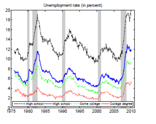
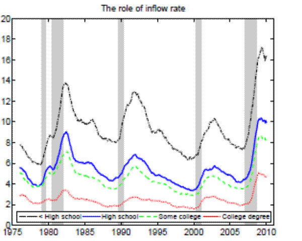
More educated individuals fare much better in the labor market than their less educated peers. For example, when the U.S. aggregate unemployment rate hit 10 percent during the recent recession, high school dropouts suffered from unemployment rates close to 20 percent, whereas college graduates experienced unemployment rates of only 5 percent. As can be inferred from Figure 1, educational attainment appears to have been a good antidote to joblessness for the whole period of data availability. Moreover, the volatility of employment decreases with education as well. Indeed, enhanced job security arguably presents one of the main benefits of education. This paper systematically and quantitatively investigates possible explanations for greater employment stability of more educated people by using recent empirical and theoretical advances in the area of worker flow analysis and search and matching models.
Notes: The sample period is 1976:01 - 2010:12. Monthly data for the working- age population constructed from CPS microdata and seasonally adjusted. Shaded areas indicat e NBER recessions.
Theoretically, differences in unemployment across education groups can arise either because the more educated find jobs faster, because the less educated get fired more often, or due to a combination of the two factors. Empirically, the worker flow analysis in this paper finds that different education groups face roughly the same unemployment outflow rate (loosely speaking, the job finding rate). What creates the remarkably divergent patterns in unemployment by education is the unemployment inflow rate (the job separation rate). Why is it then that more educated workers lose their jobs less frequently and experience lower turnover rates?
This paper provides a theoretical model in which higher educational attainment leads to greater employment stability. The model is based on vast empirical evidence showing that on-the-job training is strongly and positively related to education. As argued already by Becker (1964) higher amounts of specific training should reduce incentives of firms and workers to separate.1 We build on this insight and formalize it within a search and matching framework with endogenous separations in the spirit of Mortensen and Pissarides (1994). In our model, all new hires lack some job-specific skills, which they obtain through the process of initial on-the-job training. More educated workers engage in more complex job activities, which necessitate more initial on-the-job training. After gaining job-specific human capital, workers have less incentives to separate from their jobs, with these incentives being stronger for more educated workers. We parameterize the model by using detailed micro evidence from the Employment Opportunity Pilot Project (EOPP) survey. In particular, our empirical measure of training for each education group is based on the duration of initial on-the-job training and the productivity gap between new hires and incumbent workers.
The simulation results demonstrate that, given the observed empirical differences in initial on-the-job training, the model is able to explain the empirical regularities across education groups on job finding, separation, and unemployment rates, both in their first and second moments. This cross-sectional quantitative success of the model is quite remarkable, especially when compared to the well-documented difficulties of the canonical search and matching model to account for the main time-series properties of aggregate labor market data (Shimer, 2005 ), and thus represents the main contribution of this paper.
Perhaps the most interesting is the ability of the model to generate vast differences in the separation rate, whereas at the same time the job finding rate remains very similar across education groups. The result that on-the-job training leaves the job finding rate unaltered reflects two opposing forces. On the one hand, higher training costs lower the value of a new job, leading to less vacancy creation and a lower job finding rate. On the other hand, higher training costs reduce the probability of endogenously separating once the worker has been trained, implying a higher value of a new job and a higher job finding rate. The simulation results reveal that both effects cancel out, thus an increase in training costs leaves the job finding rate virtually unaffected. This result is important, because it cannot be obtained with standard models in the literature. Indeed, because the job creation equation represents one of the central building blocks for any search and matching model, it is very likely that alternative explanations for different unemployment dynamics by education will be inconsistent with the empirical observation of almost negligible variation in job finding rates by education.
The model in this paper can be also used to quantitatively evaluate several alternative explanations for differences in unemployment dynamics by education. In particular, the model nests the following alternative explanations: i) differences in the size of job profitability (match surplus heterogeneity); ii) differences in hiring costs; iii) differences in the frequency of idiosyncratic productivity shocks; iv) differences in the dispersion of idiosyncratic productivity shocks; and v) differences in the matching efficiency. We simulate the model under each of these alternative hypotheses and then use empirical evidence in order to discriminate between them. According to our findings, none of the economic mechanisms behind the competing explanations can generate unemployment dynamics by education that we observe in the data.2
As a final test of the theoretical mechanism embedded in our model, we provide novel empirical evidence on unemployment dynamics by required job training. In particular, we construct unemployment rates, job finding rates and separation rates by specific vocational preparation as measured in the Dictionary of Occupational Titles. This new evidence shows that occupations with higher specific vocational training experience substantially lower unemployment rates, which are predominantly due to lower separation rates. More strikingly, even after we condition for educational attainment, for example by focusing on high school graduates only, we find that higher specific vocational training leads to lower separation rates, but almost indistinguishable job finding rates, consistent with the theoretical mechanism advocated in this paper.
Our paper contributes to three strands of literature. First, it contributes to the theoretical literature of business cycle fluctuations that attempts to move beyond the representative agent framework. The aim of this literature is twofold: first, to test the plausibility of different theories by taking advantage of cross-sectional data, and second, to further our understanding of business cycle fluctuations by studying the heterogeneous impact of aggregate shocks on different demographic groups, which seems particularly relevant for fluctuations in the labor market. Relative to the existing contributions (Kydland, 1984, Gomme, Rogerson, Rupert, and Wright, 2005), we carry out our analysis within the equilibrium search and matching framework and find that the inability of this class of models to explain aggregate unemployment fluctuations at business cycle frequencies (Shimer, 2005) is not due to a failure of these models to account for fluctuations experienced by some particular education group, but instead this models' failure pertains equally to all education groups. Moreover, this paper shows that a tractable extension of the benchmark search and matching model delivers a framework that can account well for the cross-sectional differences in unemployment fluctuations by education and can be thus fruitfully utilized for studying cross-sectional labor market phenomena.
Second, our paper contributes to the theoretical literature on search and matching models with worker heterogeneity. Contributions in this literature include Gautier (2002), Albrecht and Vroman (2002), Pries (2008), Dolado, Jansen, and Jimeno (2009), Gonzalez and Shi (2010), and Krusell, Mukoyama, and Sahin (2010) . However, in these papers the worker's exit to unemployment is assumed to be exogenous, hence they cannot be used to explain why the empirical unemployment inflow rate differs dramatically by education. (Bils, Chang, and Kim (2011, 2012) allow for endogenous separations and heterogeneity in the rents from being employed; however, the latter assumption generates a substantial variation in the job finding rate and thus cannot be used to explain why the unemployment outflow rate empirically exhibits low variation by education. Relative to the existing literature, this paper provides a search and matching model with endogenous separations and on-the-job training, which can generate substantial variability in job separation rates and at the same time small differences in job finding rates, which was a challenge for existing models.
Third, our paper contributes to the empirical literature that studies cross-sectional differences in unemployment dynamics by education. Using Panel Study of Income Dynamics (PSID) data,Mincer (1991) finds that the incidence of unemployment is far more important than the reduced duration of unemployment in creating the educational differentials in unemployment rates; he attributes this finding to higher amount of on-the-job training for more educated workers. Our paper confirms this finding by using representative Current Population Survey (CPS) microdata, by constructing both duration-based and gross-flow labor market transition rates, and by controlling for possible biases (for example, duration dependence). Moreover, we use a combination of microdata and a theoretical model of equilibrium unemployment in order to interpret empirical evidence and to quantitatively discriminate among several possible explanations for observed empirical patterns.
Following this introduction, Section 2 provides some empirical evidence on unemployment, its inflows and outflows, and on-the-job training by education. Section 3 outlines the model, which is then calibrated in Section 4. Section 5 contains the main simulation results of the model and a discussion of the mechanism driving the results. In Section 6 we quantitatively explore other possible explanations for differences in unemployment dynamics by education. Novel empirical evidence on unemployment dynamics by required job training is provided in Section 7. Finally, Section 8 concludes with a discussion of possible avenues for further research. We provide data description, some further empirical results, analytical proofs, sensitivity analysis, and additional robustness checks in the Appendix.
2.1 Unemployment Rates
It is a well-known and documented empirical fact that the unemployment rate differs by education level (recall Figure 1). In the United States, the jobless rate of the least educated (high school dropouts) is roughly four times greater than that of the most educated (college graduates), and this difference has been maintained since the data are available.
| 16 years and over | 25 years and over | males, prime age (25-54) | males, prime age white | males, prime age white, married | |
| Less than high school | 12.6 | 9.0 | 9.3 | 8.5 | 7.1 |
| High school | 6.7 | 5.4 | 5.9 | 5.2 | 3.9 |
| Some college | 5.3 | 4.4 | 4.5 | 4.0 | 2.9 |
| College degree | 2.8 | 2.6 | 2.4 | 2.2 | 1.5 |
| All individuals | 6.4 | 4.9 | 5.0 | 4.5 | 3.4 |
| Ratio LHS/CD | 4.5 | 3.5 | 3.9 | 3.9 | 4.6 |
Table 1 tabulates the unemployment rate across four education groups by using the standard demographic controls (i.e., by showing the largest demographic group). As it turns out, substantial unemployment differentials across education groups represent a robust empirical finding that cannot be explained by usual demographic controls (age, gender, race, marital status). This is confirmed by results from a somewhat more formal regression analysis, which controls for individual characteristics, industry, and occupation, and includes time dummies - these results can be found in the Appendix (Table 11).
For the rest of the paper, we focus our analysis on individuals with 25 years of age and older for the following two reasons. First, by the age of 25 most individuals have presumably finished their studies, hence we avoid the possibility that our conclusions regarding unemployment properties for low educated workers could be driven by differential labor market behavior of young people. Second, further empirical exploration of unemployment rates by age reveals that young people experience somehow higher unemployment rates for all education groups, which could be related to their labor market entry that may start with an unemployment spell.3
2.2 Unemployment Flows
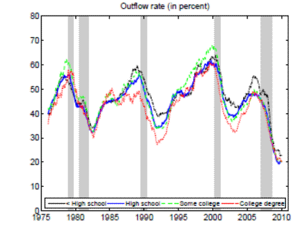
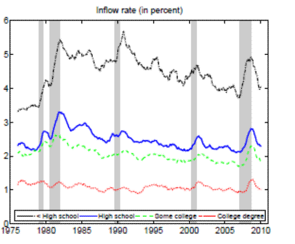
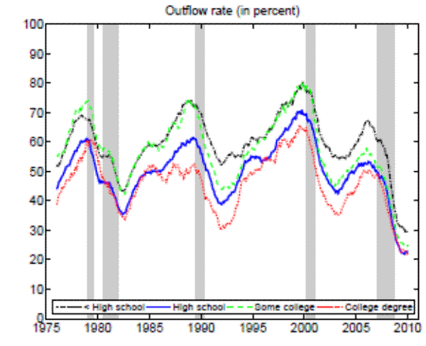
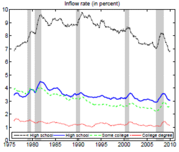
Theoretically, a higher unemployment rate may be a result of a higher probability of becoming unemployed - a higher incidence of unemployment - or a lower probability of finding a job - higher duration of the unemployment spell.4 In order to distinguish between these possibilities, we follow the recent approach in the literature by calculating empirical unemployment flows.5 In particular, we decompose unemployment rates for people with 25 years of age and over into unemployment inflow and outflow rates.6 As can be seen from Figure 2 , we find that outflow rates from unemployment are broadly similar across education
groups, whereas inflow rates differ considerably.7 Furthermore, we exploit the steady state unemployment approximation
![]() , which has been found in the literature to replicate well the actual unemployment rates (
, which has been found in the literature to replicate well the actual unemployment rates (![]() stands for the separation rate and
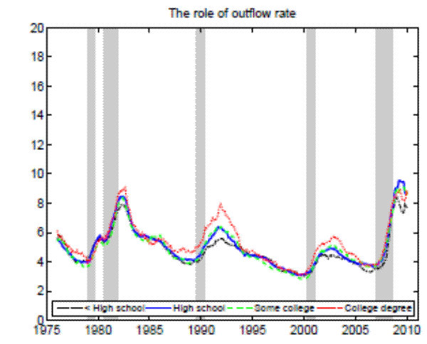
stands for the separation rate and ![]() denotes the job finding rate). In Figure 3 we construct two types of counterfactual unemployment rates to analyze separately the role of outflows and inflows in explaining the differences in unemployment rates across education groups. In particular, in the left panel of Figure 3 we calculate the counterfactual unemployment rate series for each group by taking its actual outflow rate series, but keeping the inflow rate series at the value for the aggregate economy.
Analogously, in the right panel of Figure 3 we calculate the counterfactual unemployment rate series for each group by taking its actual inflow rate series, but keeping the outflow
rate series at the value for the aggregate economy. These two counterfactuals clearly demonstrate that the observable differences in job finding rates have a negligible effect on unemployment rates, with separation rates accounting for almost all variability in unemployment rates across education
groups.8 Moreover, the observed differences in outflow rates actually go in the wrong direction as they predict (slightly) higher unemployment rates for
highly educated workers.
denotes the job finding rate). In Figure 3 we construct two types of counterfactual unemployment rates to analyze separately the role of outflows and inflows in explaining the differences in unemployment rates across education groups. In particular, in the left panel of Figure 3 we calculate the counterfactual unemployment rate series for each group by taking its actual outflow rate series, but keeping the inflow rate series at the value for the aggregate economy.
Analogously, in the right panel of Figure 3 we calculate the counterfactual unemployment rate series for each group by taking its actual inflow rate series, but keeping the outflow
rate series at the value for the aggregate economy. These two counterfactuals clearly demonstrate that the observable differences in job finding rates have a negligible effect on unemployment rates, with separation rates accounting for almost all variability in unemployment rates across education
groups.8 Moreover, the observed differences in outflow rates actually go in the wrong direction as they predict (slightly) higher unemployment rates for
highly educated workers.
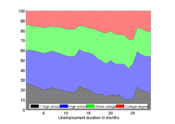
In the Appendix we further check for two possible biases regarding our conclusion that inflow rates drive the differences in unemployment rates by education. First, the procedure to calculate outflow rates might be biased due to duration dependence. Figure 11 in the Appendix illustrates that all education groups are roughly equally represented over the whole unemployment duration spectrum, hence duration dependence is not likely to bias our conclusion that outflow rates are similar by education. Second, so far we have neglected transitions in and out of the labor force. Figures 12 and 13 in the Appendix show that the findings of similar job finding rates and vastly different separation rates across education groups remain valid when considering a three-state decomposition of unemployment flows.
Notes: 12-month moving averages for individuals with 25 years of age and over.
Notes: The left panel shows the counterfactual unemployment rate series for each group by taking its actual outflow rate series, but keeping the inflow rate series at the values for the aggregate economy. The right panel shows the counterfactual unemployment rate series for each group by taking its actual inflow rate series, but keeping the outflow rate series at the values for t he aggregate economy. 12-month moving averages for individuals with 25 years of age and over.
To sum up, in order to understand why the least educated workers have unemployment rates nearly four times greater than the most educated workers, one has to identify the economic mechanisms that create a gap in their inflow rates to unemployment.
2.3 Labor Market Volatility
Table 2 summarizes volatility measures for the main labor market variables of interest. In particular, we report two sets of volatility statistics. First, absolute volatilities are defined as standard deviations of the data expressed in deviations from an HP trend with
smoothing parameter ![]() .9 Second, relative
volatilities are defined analogously, except that all variables are initially expressed in natural logarithms.10 Both sets of volatility statistics are
reported in order to facilitate the comparison with the existing literature. More precisely, on the one hand macroeconomists typically avoid taking logarithms of rates and thus prefer to report absolute volatilities. On the other hand, some of the recent literature on quantitative performance of
search and matching models puts more emphasis on relative volatilities, because what matters from the viewpoint of the canonical search and matching model are relative changes in unemployment.
.9 Second, relative
volatilities are defined analogously, except that all variables are initially expressed in natural logarithms.10 Both sets of volatility statistics are
reported in order to facilitate the comparison with the existing literature. More precisely, on the one hand macroeconomists typically avoid taking logarithms of rates and thus prefer to report absolute volatilities. On the other hand, some of the recent literature on quantitative performance of
search and matching models puts more emphasis on relative volatilities, because what matters from the viewpoint of the canonical search and matching model are relative changes in unemployment.
| Absolute volatility: |
Absolute volatility: |
Absolute volatility: |
Absolute volatility: |
Relative volatility: |
Relative volatility: |
Relative volatility: |
Relative volatility: |
|
| Less than high school | 1.78 | 1.78 | 7.62 | 0.42 | 1.99 | 18.66 | 17.45 | 9.23 |
| High school | 1.26 | 1.26 | 7.48 | 0.24 | 1.35 | 20.83 | 18.62 | 9.09 |
| Some college | 1.02 | 1.02 | 8.96 | 0.18 | 1.08 | 21.32 | 20.48 | 8.28 |
| College degree | 0.55 | 0.55 | 8.55 | 0.11 | 0.57 | 20.16 | 21.39 | 9.87 |
| All individuals | 1.05 | 1.05 | 7.49 | 0.18 | 1.12 | 20.07 | 17.99 | 7.57 |
| Ratio LHS/CD | 3.22 | 3.22 | 0.89 | 3.87 | 3.47 | 0.93 | 0.82 | 0.93 |
Our preferred volatility measure corresponds to the concept of absolute volatility. To understand why, notice that in the case of employment rates, the distinction between relative and absolute volatilities becomes immaterial.11 As the numbers in Table 2 clearly illustrate, more educated workers enjoy greater employment stability. Employment stability is arguably also the concept that matters from the welfare perspective of an individual. However, if we compare absolute and relative volatilities for unemployment rates, the numbers lead to contradictory conclusions - while absolute volatilities agree with employment volatilities by definition, relative volatilities in contrast suggest that the most educated group experiences higher unemployment volatility than the least educated group. The reason why the more educated have more volatile unemployment rates in terms of log deviations, despite having less volatile employment rates, is clearly related to their lower unemployment means.12 To avoid the distorting effect of different means on relative volatility measures, we prefer to focus on absolute volatilities. Note that the more educated experience also lower (absolute) volatility of separation rates, whereas job finding rates exhibit broadly equal variation across education groups.
2.4 On-the-Job Training
Economists have long recognized the importance of learning-by-doing, formal and informal on-the-job training for human capital accumulation. Despite the widely accepted importance of on-the-job training in theoretical work, empirical verifications of theoretical predictions remain rare, mainly due to limited data availability. Unlike with formal education, the data on training need to be obtained from scarce and frequently imperfect surveys, with considerable data imperfections being related especially to informal on-the-job training and learning-by-doing.13 Nevertheless, existing empirical studies of job training overwhelmingly suggest the presence of strong complementarities between education and training. The positive link between formal schooling and job training has been found in data from: i) the CPS Supplement of January 1983, the National Longitudinal Surveys (NLS) of Young Men, Older Men and Mature Women, and the 1980 EOPP survey by Lillard and Tan (1986); ii) the NLS of the High School Class of 1972 by Altonji and Spletzer (1991); iii) the Panel Study of Income Dynamics (PSID) by Mincer (1991); and iv) a dataset of a large manufacturing firm by Bartel (1995).
In what follows we provide some further evidence on training by education level from the 1982 EOPP survey, which will form the empirical basis for the parameterization of our model. Table 3 summarizes the main training variables of the survey with a breakdown by education.14
The EOPP survey is particularly useful to analyze training because it includes measures of both formal and informal training. This is important given that the average incidence rate of receiving initial (i.e. during first three months) formal training in our sample corresponds to 13.7 percent, while the incidence rate of receiving some type of initial training is 95.0 percent. Table 3 illustrates two relevant aspects of the data for our paper. First, nearly all new hires receive some type of initial training, regardless of their level of education. Second, there are considerable differences across education groups in terms of the duration of training received and the corresponding productivity gap (the latter is defined as the percent difference in productivity of an incumbent worker with 2 years of experience and a new hire). For example, a newly hired college graduate needs 18.2 weeks on average to become fully trained, which is nearly two times the time needed for a newly hired high school dropout.
| Less than high school | High School | Some College | College Degree | All individuals | |
| Incidence rate of initial training (mean, in percent): Formal | 9.5 | 12.0 | 18.1 | 17.9 | 13.7 |
| Incidence rate of initial training (mean, in percent): Informal by manager | 89.7 | 85.9 | 89.8 | 88.5 | 87.3 |
| Incidence rate of initial training (mean, in percent): Informal by coworkers | 56.7 | 58.0 | 62.7 | 53.5 | 58.1 |
| Incidence rate of initial training (mean, in percent): Informal by watching others | 78.1 | 75.1 | 81.0 | 73.9 | 76.3 |
| Incidence rate of initial training (mean, in percent): Some type of training | 94.0 | 94.5 | 97.0 | 95.1 | 95.0 |
| Time to become fully trained (mean, in weeks): Duration | 10.2 | 12.0 | 15.9 | 18.2 | 13.4 |
| Productivity gap (mean, in percent): Typical new hire vs. incumbent | 32.5 | 36.2 | 45.3 | 48.1 | 39.1 |
Moreover, the difference between the initial productivity and the productivity achieved by an incumbent worker increases with the education level as well, from one third to one half.
The objective of this paper is to study whether the observed differences in on-the-job training are able to explain the observed differences in unemployment rates across education groups by affecting the job destruction margin. In particular, the paper's hypothesis claims that higher investments in training reduce incentives for job destruction. However, according to the argument of Becker (1964) incentives for job destruction crucially depend on the portability of training across different jobs. As we argue below, there exist strong reasons to believe that our empirical measure of on-the-job training can indeed be interpreted as being largely job-specific and hence unportable across jobs.
First, the appropriate theoretical concept of specificity in our case is not whether a worker can potentially use his learned skills in another firm. What matters for our analysis is whether after going through an unemployment spell, a worker can still use his past training in a new job. To give an example, a construction worker might well be able to take advantage of his past training in another construction firm, but if after becoming unemployed he cannot find a new job in the construction sector and is thus forced to move to another sector, where he cannot use his past training, then his training should be viewed as specific. Industry and occupational mobility are not merely a theoretical curiosity but, as shown by Kambourov and Manovskii (2008), a notable feature of the U.S. labor market. These authors also find that industry and occupational mobility appears to be especially high when workers go through an unemployment spell.15 Similarly, by analyzing the National Longitudinal Survey of Youth (NLSY) data Lynch (1991) reaches the conclusion that on-the-job training in the United States appears to be unportable from employer to employer. In the same vein, Lynch (1992) finds that on-the-job training with the current employer increases wages, while spells of on-the-job training acquired before the current job have no impact on current wages.
Second, the EOPP was explicitly designed to measure the initial training at the start of the job (as opposed to training in ongoing job relationships), which is more likely to be of job-specific nature. Moreover, the EOPP also provides data on the productivity difference between the actual new hire during his first two weeks and the typical worker who has been in this job for two years. For the actual new hire the EOPP also reports months of relevant experience.16 Table 4 summarizes the productivity differences between the actual new hire and the typical incumbent for three age groups and also for two subsamples of new hires with at least 1 and 5 years of relevant experience. Note that one would expect to observe in the data a rapidly disappearing productivity gap (between incumbents and new hires) with rising age of workers and months of relevant experience, if this measure of on-the-job training were capturing primarily general human capital. However, the results in Table 4 indicate that initial on-the-job training remains important also for older cohorts of workers and for workers with relevant experience. Crucially for our purposes, the relative differences across education groups remain present and even increase a bit. Overall, this suggests that initial on-the-job training, at least as measured by the EOPP survey, contains primarily specific human capital.
| Less than high school | High school | Some degree | College dregree | All individuals | |
| Productivity gap (mean, in percent):16 years and over | 32.2 | 35.4 | 37.9 | 43.9 | 36.4 |
| Productivity gap (mean, in percent): 25 years and over | 24.6 | 29.3 | 37.9 | 39.3 | 31.8 |
| Productivity gap (mean, in percent): 35 years and over | 20.2 | 29.3 | 31.7 | 38.6 | 29.6 |
| Productivity gap (mean, in percent): 25 years and over and at least- 1 year of relevant experience | 22.7 | 24.5 | 34.4 | 41.7 | 28.8 |
| Productivity gap (mean, in percent): 25 years and over and at least- 5 years of relevant experience | 18.2 | 22.6 | 26.6 | 38.9 | 25.0 |
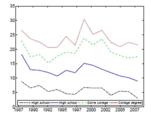
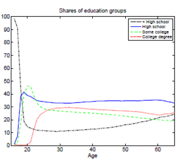
Third, Figure 4 depicts the incidence rate of formal training from the NLSY cohort.17 The analysis of these data shows that the incidence rate of formal training differs across education groups, with more educated workers receiving more training and the numbers being comparable to the ones for formal training from the EOPP survey (see Table 3). Moreover, Figure 4 shows that incidence rates of training across education groups do not exhibit a notable downward trend with aging of the 1979 NLSY cohort, consistent with the argument of the previous paragraph.
Finally, the traditional approach in the literature to distinguish between general and specific human capital has been to associate the wage return to overall work experience as an indication of the presence of general human capital, whereas the wage return to tenure has been typically interpreted as evidence of specific human capital. In an influential paper, Topel (1991) estimates that 10 years of job tenure raise the wage by over 25 percent, with wage growth being particularly rapid during an initial period of job, hence suggesting the presence of specific human capital.18 Moreover, Brown (1989) shows that firm-specific wage growth occurs almost exclusively during periods of on-the-job training, lending further support to the argument that on-the-job training is mostly specific.
3 The Model
This section presents the model, which is an extension of the canonical search and matching model with endogenous separations (Mortensen and Pissarides, 1994). In our setting workers initially lack some job-specific skills, which they obtain during a period of on-the-job training. The model allows for worker heterogeneity in terms of productivity, directly related to their formal education. Moreover, different levels of education require different amounts on-the-job training for exogenous, technological reasons, which may reflect variety in job complexity. Intuitively, more educated workers engage in more complex job activities, which necessitate a higher degree of initial on-the-job training.
3.1 Environment
The discrete-time model economy contains a finite number of segmented labor markets, indexed by
![]() , where
, where ![]() represents different levels of formal
educational attainment. Workers in each of these markets possess a certain amount of formal human capital, denoted by
represents different levels of formal
educational attainment. Workers in each of these markets possess a certain amount of formal human capital, denoted by
![]() , directly related to their education. Moreover, firms in each of these markets provide initial on-the-job training to their new hires, with the
amount of training depending on worker's education. The assumption of segmented labor markets is chosen because education is an easily observable and verifiable characteristic of workers, hence firms can direct their search towards desired education level for their new hires.19
, directly related to their education. Moreover, firms in each of these markets provide initial on-the-job training to their new hires, with the
amount of training depending on worker's education. The assumption of segmented labor markets is chosen because education is an easily observable and verifiable characteristic of workers, hence firms can direct their search towards desired education level for their new hires.19
Each segmented labor market features a continuum of measure one of risk-neutral and infinitely-lived workers. These workers maximize their expected discounted lifetime utility defined over consumption,
![]() , where
, where
![]() represents the discount factor. Workers can be either employed or unemployed. Employed workers earn wage
represents the discount factor. Workers can be either employed or unemployed. Employed workers earn wage ![]() , whereas unemployed workers have access to home production technology, which generates
, whereas unemployed workers have access to home production technology, which generates ![]() consumption units per time period. In general,
consumption units per time period. In general,
![]() also includes potential unemployment benefits, leisure, saved work-related expenditures and is net of job-searching costs. Importantly, it depends on worker's education. We abstract from
labor force participation decisions, therefore all unemployed workers are assumed to be searching for jobs.
also includes potential unemployment benefits, leisure, saved work-related expenditures and is net of job-searching costs. Importantly, it depends on worker's education. We abstract from
labor force participation decisions, therefore all unemployed workers are assumed to be searching for jobs.
A large measure of risk-neutral firms, which maximize their profits, is trying to hire workers by posting vacancies. We follow the standard approach in search and matching literature by assuming single-worker production units. In other words, each firm can post only one vacancy and for this it
pays a vacancy posting cost of ![]() units of output per time period. Here we allow this vacancy posting cost to vary across segmented labor markets, reflecting potentially more costly
searching process in labor markets that require higher educational attainment. After a match between a firm and a worker with education
units of output per time period. Here we allow this vacancy posting cost to vary across segmented labor markets, reflecting potentially more costly
searching process in labor markets that require higher educational attainment. After a match between a firm and a worker with education ![]() is formed, they first draw an idiosyncratic
productivity
is formed, they first draw an idiosyncratic
productivity ![]() . If the latter is above a certain threshold level, described more in detail below, they start producing according to the following technology:
. If the latter is above a certain threshold level, described more in detail below, they start producing according to the following technology:
3.2 Labor Markets
The matching process between workers and firms is formally depicted by the existence of a constant returns to scale matching function:
3.3 Characterization of Recursive Equilibrium
Bellman equations for the firm in labor market ![]() with required education
with required education ![]() that
is employing a trainee and a skilled worker are, respectively:
that
is employing a trainee and a skilled worker are, respectively:
Equation (4) is standard in search and matching models with endogenous separations. Observe that we also allow for exogenous separations at rate ![]() , which are
understood to be other types of separations that are not directly related to the productivity of a job. As explained above, equation (3) in addition involves the lost output
, which are
understood to be other types of separations that are not directly related to the productivity of a job. As explained above, equation (3) in addition involves the lost output ![]() that is due to initial lack of job-specific skills and the probability
that is due to initial lack of job-specific skills and the probability ![]() of becoming a skilled worker.
of becoming a skilled worker.
![]() denotes expectations conditioned on the current values of
denotes expectations conditioned on the current values of ![]() and
and
![]() . Note that at any point in time, a firm can also decide to fire its employee and become inactive in which case it obtains a zero payoff. The firm optimally chooses to endogenously separate
at and below the reservation productivities
. Note that at any point in time, a firm can also decide to fire its employee and become inactive in which case it obtains a zero payoff. The firm optimally chooses to endogenously separate
at and below the reservation productivities
![]() and
and
![]() , which are implicitly defined as the maximum values that satisfy:
, which are implicitly defined as the maximum values that satisfy:
| (5) | ||
| (6) |
The free entry condition equalizes the costs of posting a vacancy (recall that ![]() is per period vacancy posting cost and
is per period vacancy posting cost and
![]() is the expected vacancy duration) with the expected discounted benefit of getting an initially untrained worker:
is the expected vacancy duration) with the expected discounted benefit of getting an initially untrained worker:
The unemployed worker enjoys utility ![]() and with probability
and with probability
![]() meets with a vacancy:
meets with a vacancy:
| (8) |
Note that the unemployed worker always starts a job as a trainee, due to the initial lack of job-specific skills. 21 Bellman equations for the worker are analogous to the firm's ones, with his outside option being determined by the value of being unemployed:
| (9) | ||
| (10) | ||
Under the generalized Nash wage bargaining rule the worker gets a fraction ![]() of total match surplus, defined as:
of total match surplus, defined as:
for the job with a trainee and a skilled worker, respectively. Hence:
Observe that the above equations imply that the firm and the worker both want a positive match surplus. Therefore, there is a mutual agreement on when to endogenously separate. From the above surplus-splitting equations it is straightforward to show that the wage equations are given by:
for the trainee and the skilled worker, respectively. The wage equations imply that the worker and the firm share the cost of training in accordance with their bargaining powers.
The model features a recursive equilibrium, with its solution being determined by equations (1)-(12). The solution of the model consists of equilibrium labor market tightness
![]() and reservation productivities
and reservation productivities
![]() and
and
![]() . Next, the following proposition establishes an important neutrality result.
. Next, the following proposition establishes an important neutrality result.
Moreover, the free entry condition can be written in terms of the surplus as:
 |
||
 |
Substituting recursively, it is straightforward to check that the solution of the model is equivalent for
The usefulness of Proposition 1 will become clear in the following two sections with calibration and numerical results of the model. In particular, the proposition's result enables a transparent comparison of the model results across different education groups
![]() , with the only parameters affecting results being on-the-job training parameters. Notably, by using the proposition we avoid changing the surpluses by magnifying the difference between the
firm's output and the value of being unemployed. We believe that the model's implications when changing the value of being unemployed relative to output have been well explored in the recent literature.22 Indeed, by assuming that more educated workers enjoy higher match surplus (with
, with the only parameters affecting results being on-the-job training parameters. Notably, by using the proposition we avoid changing the surpluses by magnifying the difference between the
firm's output and the value of being unemployed. We believe that the model's implications when changing the value of being unemployed relative to output have been well explored in the recent literature.22 Indeed, by assuming that more educated workers enjoy higher match surplus (with ![]() being lower relative to output than
in the case of less educated workers) it is well documented that the model would predict a decrease in the unemployment and the separation rate, but at the same time it would also predict an increase in the job finding rate. The latter prediction strongly contradicts the empirical evidence across
education groups, as documented in Section 2. Further discussion of these issues together with some empirical evidence justifying the assumptions of proportionality in
being lower relative to output than
in the case of less educated workers) it is well documented that the model would predict a decrease in the unemployment and the separation rate, but at the same time it would also predict an increase in the job finding rate. The latter prediction strongly contradicts the empirical evidence across
education groups, as documented in Section 2. Further discussion of these issues together with some empirical evidence justifying the assumptions of proportionality in ![]() and
and ![]() is provided in the next section.
is provided in the next section.
With the obtained solution of the model we can generate numerical results by simulating it, using the law of motion for trainees and skilled workers. The mass of trainees next period with idiosyncratic productivity ![]() is given by:
is given by:
![\displaystyle \mathbbm{1}{\left\{a_j>\tilde{a}^T(H,A')\right\}} \left[ (1-\delta) (1-\phi_h) \sum_{i=1}^{m} \pi^a_{ij} n^T(a_i) + p(\theta(H,A)) \pi^a_{j} u(H,A) \right]. %\quad \forall j.](img105.gif) |
First notice that if
Similarly, the mass of skilled workers next period with idiosyncratic productivity ![]() is given by:
is given by:
![\displaystyle \mathbbm{1}{\left\{a_j>\tilde{a}^S(H,A')\right\}}\left[ (1-\delta) \sum_{i=1}^{m} \pi^a_{ij} n^S(a_i) + (1-\delta) \phi_h \sum_{i=1}^{m} \pi^a_{ij} n^T(a_i) \right]. % \quad \forall j.](img109.gif) |
Again, notice that if
Finally, the aggregate employment rate ![]() and unemployment rate
and unemployment rate ![]() are defined
as:
are defined
as:
 |
||
respectively. Labor productivity is defined as total production (
 |
3.4 Efficiency
The canonical search and matching model features search externalities. It is well-known that the equilibrium of this model yields a socially efficient outcome, provided that the Hosios condition is satisfied (Hosios, 1990). This condition equalizes the worker's bargaining power to the elasticity of the matching function with respect to unemployment. Does the same condition also apply to our model or is there some role for policy?
The proof of the above proposition is given in the Appendix. Hence, the standard Hosios condition applies also to our setting where workers are initially untrained. In other words, there are no additional inefficiencies specific to our model, except from the standard search externalities. Therefore, differential unemployment outcomes, which are related to differential training requirements, are efficient in our model if the Hosios condition is satisfied. This result is intuitive, because training requirements in our model are merely a technological constraint. Finally, we show in the Appendix that the job destruction is maximized when the Hosios condition holds.23
4 Calibration
We proceed by calibrating the model. First, we discuss the calibration of parameter values that are consistent with empirical evidence at the aggregate level. Second, we specify the on-the-job training parameter values that are specific to each education group.
4.1 Parameter Values at the Aggregate Level
The model is simulated at monthly frequency. Table 5 summarizes the parameter values at the aggregate level.
| Parameter | Interpretation | Value | Rationale |
| Discount factor | 0.9966 | Interest rate 4% p.a. | |
| Matching efficiency | 0.45 | Job finding rate 45.3% (CPS) | |
| Elasticity of the matching function | 0.5 | Petrongolo and Pissarides (2001) | |
| Worker's bargaining power | 0.5 | Hosios condition | |
| Vacancy posting cost | 0.106 | 1982 EOPP survey | |
| Value of being unemployed | 0.82 | See text | |
| Standard deviation for log aggregate productivity | 0.0064 | Labor productivity (BLS) | |
| Autoregressive parameter for log aggregate productivity | 0.98 | Labor productivity (BLS) | |
| Mean log idiosyncratic productivity | 0 | Normalization | |
| Standard deviation for log idiosyncratic productivity | 0.249 | Separation rate 2.24% (CPS) | |
| Probability of changing idiosyncratic productivity | 0.3333 | Fujita ad Ramey | |
| Exogenous separation rate | 0.0075 | JOLTS data | |
| Probability of training upgrade | 0.3226 | 1982 EOPP survey | |
| Training costs | 0.196 | 1982 EOPP survey | |
| Worker's productivity | 1 | Normalization |
The value of the discount factor is consistent with an annual interest rate of four percent. The efficiency parameter ![]() in the matching function targets a mean monthly job finding
rate of 45.3 percent, consistent with the CPS microevidence for people with 25 years and over as described in Section 2.2. For the elasticity of the Cobb-Douglas matching function with respect to unemployment we draw from the evidence reported in Petrongolo and Pissarides (2001) and
accordingly set
in the matching function targets a mean monthly job finding
rate of 45.3 percent, consistent with the CPS microevidence for people with 25 years and over as described in Section 2.2. For the elasticity of the Cobb-Douglas matching function with respect to unemployment we draw from the evidence reported in Petrongolo and Pissarides (2001) and
accordingly set
![]() . Absent any further microevidence, we follow most of the literature and put the workers' bargaining power equal to
. Absent any further microevidence, we follow most of the literature and put the workers' bargaining power equal to ![]() .24 As we show in Section 3.4, this guarantees efficiency of the
equilibrium, consistent with the Hosios condition.
.24 As we show in Section 3.4, this guarantees efficiency of the
equilibrium, consistent with the Hosios condition.
For the parameterization of the vacancy posting cost we take advantage of the EOPP data, which contain information on vacancy duration and hours spent during the recruitment process.25 In our sample it took on average 17.8 days to fill the vacancy, with 11.3 hours being spent during the whole recruitment process.26 Note that the expected recruitment cost in the model is equal to the product of the flow vacancy posting cost and the expected duration of the vacancy,
![]() . Hence, we have on a monthly basis
. Hence, we have on a monthly basis
![]() , which gives us the flow vacancy posting cost
, which gives us the flow vacancy posting cost ![]() .27 The vacancy posting cost equals 10.5 percent of average worker's productivity in our simulated model, which also appears to be broadly consistent with
other parameter values for the vacancy posting cost used in the literature.28
.27 The vacancy posting cost equals 10.5 percent of average worker's productivity in our simulated model, which also appears to be broadly consistent with
other parameter values for the vacancy posting cost used in the literature.28
The flow value of non-market activities ![]() in general consists of: i) unemployment insurance benefits; ii) home production and self-employment; iii) value of leisure and disutility of
work; iv) expenditures saved by not working; and v) is net of job-searching costs. The literature has demonstrated that this parameter value crucially affects the results of the model. Low values of
in general consists of: i) unemployment insurance benefits; ii) home production and self-employment; iii) value of leisure and disutility of
work; iv) expenditures saved by not working; and v) is net of job-searching costs. The literature has demonstrated that this parameter value crucially affects the results of the model. Low values of ![]() , such as in Shimer (2005) who uses
, such as in Shimer (2005) who uses ![]() , imply large surpluses and low volatilities of labor market variables. High values of
, imply large surpluses and low volatilities of labor market variables. High values of ![]() , such as in Hagedorn and Manovskii (2008) who use
, such as in Hagedorn and Manovskii (2008) who use ![]() , instead generate high volatilities, but as shown by
Costain and Reiter (2008) also imply unrealistic responses of unemployment levels to policy changes in unemployment benefits. Here, we decided to choose an intermediate level of
, instead generate high volatilities, but as shown by
Costain and Reiter (2008) also imply unrealistic responses of unemployment levels to policy changes in unemployment benefits. Here, we decided to choose an intermediate level of ![]() ,
which imply 81.2 percent of average labor productivity in our simulated model. As shown in the Appendix, our main results remain unaffected if we set
,
which imply 81.2 percent of average labor productivity in our simulated model. As shown in the Appendix, our main results remain unaffected if we set ![]() as in Hall and Milgrom (2008) and Pissarides (2009)
and Hall and Milgrom (2008) and Pissarides (2009).
as in Hall and Milgrom (2008) and Pissarides (2009)
and Hall and Milgrom (2008) and Pissarides (2009).
Parameters for the Markov chain governing the aggregate productivity process are calibrated to match the cyclical properties of the quarterly average U.S. labor productivity between 1976 and 2010.29 After taking logs and deviations from an HP trend with smoothing parameter ![]() , the standard deviation of quarterly
labor productivity is equal to 0.018 and its quarterly autocorrelation is equal to 0.90. We apply the Rouwenhorst (1995) method for finite state Markov-chain approximations of AR(1) processes, which has been found to generate accurate approximations to highly persistent processes (Kopecky and Suen 2010).
, the standard deviation of quarterly
labor productivity is equal to 0.018 and its quarterly autocorrelation is equal to 0.90. We apply the Rouwenhorst (1995) method for finite state Markov-chain approximations of AR(1) processes, which has been found to generate accurate approximations to highly persistent processes (Kopecky and Suen 2010).
In choosing the Markov chain for the idiosyncratic productivity process, we follow the standard assumption in the literature by assuming that idiosyncratic shocks are independent draws from a lognormal distribution with parameters ![]() and
and ![]() . As in Fujita and Ramey (2012), these draws occur on average every quarter (
. As in Fujita and Ramey (2012), these draws occur on average every quarter (
![]() ), governing the persistence of the Markov chain. In order to determine the parameters of the lognormal distribution and the exogenous separation rate we match the empirical
evidence on separation rates. The CPS microevidence for people with 25 years of age and over gives us a mean monthly inflow rate to unemployment of 2.24 percent. The recent Job Openings and Labor Turnover Survey (JOLTS) data, available from December 2000 onwards, tell us that the mean monthly
layoff rate is equal to 1.5 percent. The layoffs in JOLTS data correspond to involuntary separations initiated by the employer, hence we take these to be endogenous separations. Accordingly, we set the exogenous monthly separation rate to
), governing the persistence of the Markov chain. In order to determine the parameters of the lognormal distribution and the exogenous separation rate we match the empirical
evidence on separation rates. The CPS microevidence for people with 25 years of age and over gives us a mean monthly inflow rate to unemployment of 2.24 percent. The recent Job Openings and Labor Turnover Survey (JOLTS) data, available from December 2000 onwards, tell us that the mean monthly
layoff rate is equal to 1.5 percent. The layoffs in JOLTS data correspond to involuntary separations initiated by the employer, hence we take these to be endogenous separations. Accordingly, we set the exogenous monthly separation rate to
![]() percent, and adjust
percent, and adjust ![]() in order that the simulated data
generate mean monthly inflow rates to unemployment of 2.24 percent. The parameter
in order that the simulated data
generate mean monthly inflow rates to unemployment of 2.24 percent. The parameter ![]() is normalized to zero.
is normalized to zero.
We select parameters regarding on the-job-training from the 1982 EOPP survey as summarized in Table 3 of Section 2.4. To calibrate the duration of on-the-job training we consider the time to become fully trained in months. In particular, under the baseline
calibration we parameterize the average duration of on-the-job training to 3.10 months (
![]() ), which yields the value for
), which yields the value for ![]() equal to
equal to ![]() . To calibrate the extent of on-the-job training we use the average productivity gap between a typical new hire and a typical fully trained worker. In reality, we would expect that workers obtain
job-specific skills in a gradual way, i.e. shrinking the productivity gap due to lack of skills proportionally with the time spent on the job. Our parameterization of training costs for the aggregate economy,
. To calibrate the extent of on-the-job training we use the average productivity gap between a typical new hire and a typical fully trained worker. In reality, we would expect that workers obtain
job-specific skills in a gradual way, i.e. shrinking the productivity gap due to lack of skills proportionally with the time spent on the job. Our parameterization of training costs for the aggregate economy,
![]() , implies that trainees are on average 19.6 percent less productive than skilled workers. This is consistent with an average initial gap of 39.1 percent, which is then
proportionally diminishing over time. Finally, the worker's productivity parameter
, implies that trainees are on average 19.6 percent less productive than skilled workers. This is consistent with an average initial gap of 39.1 percent, which is then
proportionally diminishing over time. Finally, the worker's productivity parameter ![]() is normalized to one.
is normalized to one.
4.2 Parameter Values Specific to Education Groups
Next we turn to parameterizing the model across education groups. We keep fixed all the parameter values at the aggregate level as reported in Table 5, with the only exception being the training parameters (![]() and
and ![]() ). In particular, we assume that
). In particular, we assume that ![]() and
and ![]() , making applicable the neutrality result of Proposition 1, according to which the parameterization for
, making applicable the neutrality result of Proposition 1, according to which the parameterization for ![]() is irrelevant. We argue below that this is not only desirable from the model comparison viewpoint as we can completely isolate the effects of on-the-job training, but it is also a reasonable thing to do
given available empirical evidence. Note also that a neutrality result similar to Proposition 1 would obtain if we were to assume a standard utility function in macroeconomic literature, featuring disutility of labor and offsetting income and substitution
effects.30
is irrelevant. We argue below that this is not only desirable from the model comparison viewpoint as we can completely isolate the effects of on-the-job training, but it is also a reasonable thing to do
given available empirical evidence. Note also that a neutrality result similar to Proposition 1 would obtain if we were to assume a standard utility function in macroeconomic literature, featuring disutility of labor and offsetting income and substitution
effects.30
Regarding the parameterization of parameter ![]() , recall that this parameter should capture several elements, including unemployment insurance benefits, home production, disutility of
work, expenditures saved by not working, and job-searching costs. Intuitively, higher educational attainment could lead to higher
, recall that this parameter should capture several elements, including unemployment insurance benefits, home production, disutility of
work, expenditures saved by not working, and job-searching costs. Intuitively, higher educational attainment could lead to higher ![]() through all of the mentioned elements. More educated
workers typically earn higher salaries and are hence also entitled to higher unemployment insurance benefits (albeit the latter are usually capped at some level). Higher educational attainment presumably not only increases market productivity, but also home production, which incorporates the
possibility of becoming self-employed. Jobs requiring more education could be more stressful, leading to higher disutility of work, and might require higher work-related expenditures (e.g., commuting, meals, clothing). Finally, more educated workers might be able to take advantage of more efficient
job-searching methods, lowering their job-searching costs. Overall, there seems to be little a priori justification to simply assume that more educated workers enjoy higher job surplus.
through all of the mentioned elements. More educated
workers typically earn higher salaries and are hence also entitled to higher unemployment insurance benefits (albeit the latter are usually capped at some level). Higher educational attainment presumably not only increases market productivity, but also home production, which incorporates the
possibility of becoming self-employed. Jobs requiring more education could be more stressful, leading to higher disutility of work, and might require higher work-related expenditures (e.g., commuting, meals, clothing). Finally, more educated workers might be able to take advantage of more efficient
job-searching methods, lowering their job-searching costs. Overall, there seems to be little a priori justification to simply assume that more educated workers enjoy higher job surplus.
To proceed further, we turn to empirical evidence reported in Aguiar and Hurst (2005), who among other things measure food consumption and food expenditure changes during unemployment. Focusing on food items (which include eating in restaurants) is a bit restrictive for our purposes, but the
results are nevertheless illustrative. Aguiar and Hurst (2005) report their estimates separately for the whole sample and for the "low-education" subsample, which consist of individuals with 12 years or less of schooling. They find that during unemployment food expenditure falls by 19 percent
for the whole sample and by 21 percent for the low-education sample, with the difference not being statistically significant. The drop in food consumption amounts to 5 percent for the whole sample and 4 percent for the low-education sample, with the numbers being statistically significant from
zero, but not from each other.31 Based on this micro evidence and the reasoning given above, we take ![]() to be a reasonable assumption. Results from robustness checks on this assumption are provided in the Appendix.
to be a reasonable assumption. Results from robustness checks on this assumption are provided in the Appendix.
The proportionality assumption on flow vacancy posting cost would follow directly if we were to assume that hiring is a labor intensive activity as in Shimer (2009). Moreover, the textbook matching model also assumes proportionality of hiring costs to productivity (Pissarides, 2000). Nevertheless, we perform the sensitivity analysis of the quantitative results with respect to different specification of vacancy posting cost and report them in the Appendix.
For the parameters regarding on-the-job training we refer the reader to Table 3 in Section 2.4. Moreover, we will report all on-the-job training parameter values for different education groups in the tables with simulation results.
5 Simulation results
The main results of the paper are presented in this section. First, we report baseline simulation results for the aggregate economy. Second, the model is solved and simulated for each education group. This exercise is done by changing the parameters ![]() and
and ![]() related to on-the-job training for each education group, while keeping the rest of parameters fixed at the
aggregate level. Finally, we discuss the main mechanism of the model, by exploring how simulation results depend on each training parameter. This section reports simulation results with the calibration for the age group of 25 years and older. As shown in the Appendix, our conclusions remain
unaffected if we calibrate the model for the whole working-age population.
related to on-the-job training for each education group, while keeping the rest of parameters fixed at the
aggregate level. Finally, we discuss the main mechanism of the model, by exploring how simulation results depend on each training parameter. This section reports simulation results with the calibration for the age group of 25 years and older. As shown in the Appendix, our conclusions remain
unaffected if we calibrate the model for the whole working-age population.
5.1 Baseline Simulation Results
We begin by simulating the model, parameterized at the average aggregate level for duration of training and training costs (
![]() and
and
![]() ). Table 6 reports the baseline simulation results together
with the actual data moments for the United States during 1976-2010. In particular, we report means, absolute and relative volatilities for the key variables of interest. The reported model statistics are means of statistics computed from 100 simulations. In each simulation, 1000 monthly
observations for all variables are obtained. The first 580 months are discarded and the last 420 months, corresponding to data from 1976:01 to 2010:12, are used to compute the statistics in the same way as we do for the data. In order to assess the precision of the results, standard deviations of
simulated statistics are computed across simulations.
). Table 6 reports the baseline simulation results together
with the actual data moments for the United States during 1976-2010. In particular, we report means, absolute and relative volatilities for the key variables of interest. The reported model statistics are means of statistics computed from 100 simulations. In each simulation, 1000 monthly
observations for all variables are obtained. The first 580 months are discarded and the last 420 months, corresponding to data from 1976:01 to 2010:12, are used to compute the statistics in the same way as we do for the data. In order to assess the precision of the results, standard deviations of
simulated statistics are computed across simulations.
| Panel A: U.S. data, 1976 - 2010: Mean | - | 95.11 | 4.89 | 45.26 | 2.24 |
| Panel A: U.S. data, 1976 - 2010: Absolute volatility | - | 1.05 | 1.05 | 7.49 | 0.18 |
| Panel A: U.S. data, 1976 - 2010: Relative volatility | 1.78 | 1.12 | 20.07 | 17.99 | 7.57 |
| Panel B: Baseline simulation results: Mean | - | 95.14 | 4.86 | 45.24 | 2.25 |
| Panel B: Baseline simulation results: Mean (std. deviation) | (0.61) | (0.61) | (2.39) | (0.16) | |
| Panel B: Baseline simulation results: Absolute volatility | - | 0.80 | 0.80 | 3.22 | 0.23 |
| Panel B: Baseline simulation results: Absolute volatility (std. deviation) | (0.28) | (0.28) | (0.64) | (0.07) | |
| Relative volatility | 1.78 | 0.85 | 15.47 | 7.28 | 9.64 |
| Panel B: Baseline simulation results :Relative volatility (std. deviation) | (0.34) | (0.31) | (3.55) | (1.65) | (2.18) |
The baseline simulation results show that the model performs reasonably well at the aggregate level. It essentially hits the empirical means of the unemployment rate, the job finding rate and the separation rate by construction of the exercise. More notably, it also mirrors well the empirical volatilities. Two main reasons why the model does not suffer from an extreme unemployment volatility puzzle as in Shimer (2005) relate to a bit higher flow value of being unemployed and the inclusion of endogenous separations.32 The latter are also the reason why the model matches the volatility of the separation rate quite well.33 The model underpredicts the volatility of the job finding rate and to a somewhat lesser extent the volatility of the unemployment rate, which should not be surprising given that in this model productivity shocks are the only cause of fluctuations in vacancies.34
5.2 Unemployment Rates across Education Groups
Next, we turn to the simulation results across different education groups. We keep fixed all the parameter values at the aggregate level and only vary the training parameters across education groups. Table 7 shows the simulation results for the means. As we can see, the model is able to explain the differences in unemployment rates across education groups that we observe in the data. In particular, the ratio of unemployment rates of the least educated group to the most educated group is 3.5 in the data and 3.4 in the model. Moreover, the model accounts for the observable differences in separation rates across groups, while keeping similar job finding rates. The ratio of separation rates of the least educated group to the most educated group is 4.1 in the data and 3.6 in the model. In general, the greater is the degree of on-the-job training (longer training periods and higher productivity gaps), the lower is the separation rate and the lower is the unemployment rate. Therefore, the observed variation in training received across education groups can explain most of the observed differences in separation rates and unemployment rates.
| Data: |
Data: |
Data: |
Parameters: |
Parameters: |
Model: |
Model: |
Model: |
|
| Less than high school | 8.96 | 46.85 | 4.45 | 2.35 | 0.163 | 7.93 | 45.51 | 3.83 |
| Less than high school (std. deviation) | (0.75) | (2.08) | (0.21) | |||||
| High school | 5.45 | 45.02 | 2.48 | 2.78 | 0.181 | 6.09 | 45.53 | 2.88 |
| High school (std. deviation) | (0.71) | (2.38) | (0.20) | |||||
| Some college | 4.44 | 46.34 | 2.05 | 3.67 | 0.227 | 3.02 | 45.08 | 1.36 |
| Some college (std. deviation) | (0.32) | (2.35) | (0.08) | |||||
| College degree | 2.56 | 42.80 | 1.09 | 4.19 | 0.240 | 2.35 | 45.27 | 1.06 |
| College degree (std. deviation) | (0.25) | (2.38) | (0.05) |
Table 8 presents a more detailed view of the results, offering a breakdown of separation rates and employment rates for trainees and for skilled workers. As it can be seen, separation rates of trainees are roughly similar across education groups and trainees represent a small share of employment for all four education groups. Therefore, differences in separation rates for skilled workers are the main reason why more educated workers enjoy lower separation rates.
| Less than high school | 3.83 | 7.83 | 3.63 | 92.07 | 7.47 | 84.60 |
| High school | 2.88 | 7.69 | 2.65 | 93.91 | 6.59 | 87.32 |
| Some college | 1.36 | 7.32 | 1.18 | 96.98 | 4.05 | 92.94 |
| College degree | 1.06 | 7.13 | 0.89 | 97.65 | 3.54 | 94.11 |
| All individuals | 2.25 | 7.59 | 2.02 | 95.14 | 5.70 | 89.45 |
5.3 Unemployment Volatility across Education Groups
Panel A of Table 9 reports the simulation results for absolute volatilities. As mentioned in Section 5.1, the model underpredicts the volatilities of the job finding and the unemployment rates. This property of the model is also inherited here. Nevertheless, the model replicates well the relative differences in volatilities across education groups. In the data, the volatility of the unemployment rate for high school dropouts is 3.2 times higher than the corresponding volatility for college graduates, whereas the same ratio in the model stands at 3.7. Something similar is true for volatilities of separation rates (the ratio is 3.9 in the data and 5.5 in the model), where additionally the model also explains volatility levels quite well. The model can also account for the observed similar values of volatilities in job finding rates across education groups.
Panel B of Table 9 reports the simulation results for relative volatilities. The model succeeds in replicating the ratio of relative employment volatility of the least educated group to the most educated group (the ratio is 3.5 in the data and 3.9 in the model). This finding is not surprising given the results of Panel A of Table 9, which show that the model is able to replicate the ratio of absolute employment volatility. The model also accounts well for the empirical finding that relative volatilities in unemployment, job finding, and separation rates are similar across education groups.
5.4 Unemployment Dynamics across Education Groups
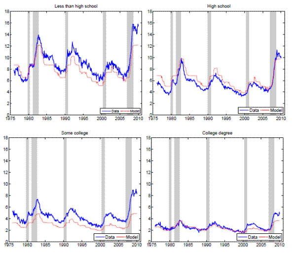
To provide another view of the model's results we conduct the following experiment. Using the model's original solution for the aggregate economy and the actual data on the aggregate unemployment rate we back out the implied realizations of the aggregate productivity innovations. Then, we feed this implied aggregate productivity series to the model's original solution for each education group. The simulated unemployment rate series for each group are shown in Figure 5, together with the actual unemployment rates. Again, the model replicates the data remarkably well, both in terms of capturing the differences in means and volatilities across groups.
| Data: |
Data: |
Data: |
Data: |
Parameters: |
Parameters |
Model: |
Model: |
Model: |
Model: |
|
| Panel A: Absolute volatilities: Less than high school | 1.78 | 1.78 | 7.62 | 0.42 | 2.35 | 0.163 | 1.14 | 1.14 | 3.07 | 0.34 |
| Panel A: Absolute volatilities: Less than high school (std. deviation) | (0.28) | (0.28) | (0.63) | (0.07) | ||||||
| Panel A: Absolute volatilities: High school | 1.26 | 1.26 | 7.48 | 0.24 | 2.78 | 0.181 | 0.91 | 0.91 | 3.07 | 0.27 |
| Panel A: Absolute volatilities: High school (std. deviation) | (0.27) | (0.27) | (0.57) | (0.07) | ||||||
| Panel A: Absolute volatilities: Some college | 1.02 | 1.02 | 8.96 | 0.18 | 3.67 | 0.227 | 0.48 | 0.48 | 3.34 | 0.12 |
| Panel A: Absolute volatilities: Some college (std. deviation) | (0.14) | (0.14) | (0.54) | (0.03) | ||||||
| Panel A: Absolute volatilities: College degree | 0.55 | 0.55 | 8.55 | 0.11 | 4.19 | 0.240 | 0.31 | 0.31 | 3.30 | 0.06 |
| Panel A: Absolute volatilities: College degree (std. deviation) | (0.12) | (0.12) | (0.68) | (0.02) | ||||||
| Panel B: Relative volatilities: Less than high school | 1.99 | 18.66 | 17.45 | 9.23 | 2.35 | 0.163 | 1.25 | 13.65 | 6.88 | 8.55 |
| Panel B: Relative volatilities: Less than high school (std. deviation) | (0.32) | (2.87) | (1.47) | (1.66) | ||||||
| Panel B: Relative volatilities: High school | 1.35 | 20.83 | 18.62 | 9.09 | 2.78 | 0.181 | 0.98 | 14.36 | 6.86 | 9.04 |
| Panel B: Relative volatilities: High school (std. deviation) | (0.30) | (2.96) | (1.43) | (1.79) | ||||||
| Panel B: Relative volatilities: Some college | 1.08 | 21.32 | 20.48 | 8.28 | 3.67 | 0.227 | 0.49 | 14.67 | 7.55 | 8.20 |
| Panel B: Relative volatilities: Some college (std. deviation) | (0.15) | (2.93) | (1.35) | (1.75) | ||||||
| Panel B: Relative volatilities: College degree | 0.57 | 20.16 | 21.39 | 9.87 | 4.19 | 0.240 | 0.32 | 12.13 | 7.47 | 5.51 |
| Panel B: Relative volatilities: College degree | (0.13) | (3.21) | (1.69) | (1.70) |
5.5 Discussion of the Model's Mechanism
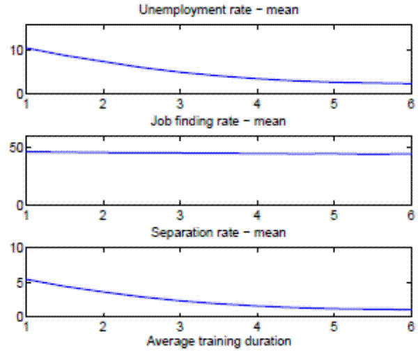
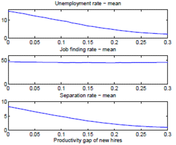
In order to highlight the mechanism at work in our model, two more exercises are conducted. In particular, we analyze separately the effects of training duration and productivity gap of new hires to demonstrate that both of them quantitatively play almost equally important roles for our results. In the left panel of Figure 6 we study the role of the average duration of on-the-job training, keeping the rest of the parameters constant at the aggregate level. Analogously, the right panel of Figure 6 studies the role of the productivity gap of new hires, keeping the rest of the parameters constant at the aggregate level. In both cases, we observe a decrease in the mean of the unemployment rate as we increase the degree of on-the-job training (longer training periods and higher productivity gaps). This decrease in the unemployment rate is completely driven by the decrease in the separation rate, given that the job finding rate remains roughly constant as we vary the degree of on-the-job training.35
Let's consider first why the job finding rate virtually does not move with the average duration of on-the-job training. One would expect that an increase in the average duration
Notes: Actual unemployment rates are quarterly averages of monthly se asonally-adjusted data con- structed from CPS microdata. The simulated unemployment rates a re generated by solving and simu- lating the model for each education group using the implied realization s of the aggregate productivity innovations as explained in the text.
of on-the-job training reduces the value of a new job, since the worker spends more time being less productive. Consequently, firms' incentives to post vacancies should decrease, leading to a decrease in the job finding rate. However, an increase in the average duration of on-the-job training also reduces the probability of separating endogenously once the worker becomes skilled. This second effect increases the value of a new job, and hence incentives for vacancy posting go up. It turns out that these two effects cancel out and the job finding rate hence remains almost unaffected. The same reasoning holds for the productivity gap of new hires, which measures the extent of on-the-job training. Again, we have two effects at work, which cancel each other out - a higher extent of on-the-job training by itself decreases the value of a new job, but at the same time the latter increases through lower endogenous separations of skilled workers.
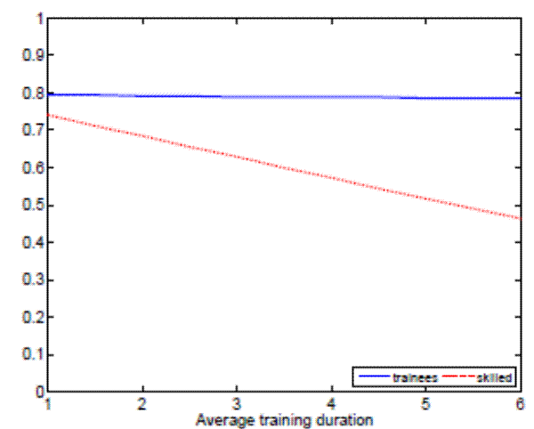
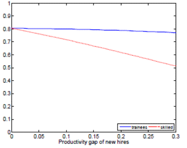
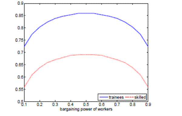
In order to understand why separation rates decrease with the degree of on-the-job training, we analyze match incentives to separate. Figure 7 shows the reservation productivities for trainees and skilled workers for different degrees of on-the-job training. As we can see, investments in match-specific human capital do not significantly affect the
Notes: Statistics are means (in percent) across 100 simulations. The left p anel studies the role of the average duration of on-the-job training, keeping the rest of par ameters constant at the aggregate level. The right panel studies the role of the productivity gap of new hires , keeping the rest of parameters constant at the aggregate level.
incentives of trainees to separate, while they clearly reduce skilled workers' incentives to separate. The intuition for this result is that skilled workers know that upon a job loss they will have to undergo first, a period of searching for a new job and second, a period of on-the-job training with a lower wage. Hence, reservation productivity levels drop for skilled workers as we increase the degree of on-the-job training, implying a lower rate of endogenous separations.
Notes: The left panel plots reservation productivities for trainees and sk illed workers for different training durations, keeping the rest of parameters constant at the aggr egate level. The right panel plots reservation productivities for trainees and skilled workers for different produc tivity gaps of new hires, keeping the rest of parameters constant at the aggregate level.
6 Evaluating Other Potential Explanations
This section evaluates the plausibility of other potential explanations for differential unemployment dynamics by education. In particular, our model can encompass the following alternative hypotheses: i) differences in the size of match surplus ; ii) differences in hiring costs; iii) differences in frequency of idiosyncratic productivity shocks; iv) differences in dispersion of idiosyncratic productivity shocks; and v) differences in matching efficiency. We simulate the model under each of these alternative hypotheses and then confront the obtained simulation results with empirical evidence. In particular, for these simulations we use the parameter values for the aggregate level as given in Table 5, whereas across education groups we only allow to vary the parameter that is crucial for each alternative hypothesis. This helps us to highlight economic mechanisms behind the alternative hypotheses. Simulations results are summarized in Table 10.
| Panel A: U.S. data, 1976 - 2010: Less than high school | 8.96 | 46.85 | 4.45 |
| Panel A: U.S. data, 1976 - 2010: High school | 5.45 | 45.02 | 2.48 |
| Panel A: U.S. data, 1976 - 2010: Some college | 4.44 | 46.34 | 2.05 |
| Panel A: U.S. data, 1976 - 2010: College degree | 2.56 | 42.80 | 1.09 |
| Panel B: Size of Match Surplus:
|
14.37 | 29.28 | 4.61 |
| Panel B: Size of Match Surplus:
|
7.12 | 39.31 | 2.89 |
| Panel B: Size of Match Surplus:
|
3.89 | 49.20 | 1.95 |
| Panel B: Size of Match Surplus:
|
2.43 | 58.29 | 1.44 |
| Panel C: Hiring Costs:
|
8.76 | 55.26 | 5.19 |
| Panel C: Hiring Costs:
|
5.13 | 46.06 | 2.42 |
| Panel C: Hiring Costs:
|
3.58 | 40.83 | 1.48 |
| Panel C: Hiring Costs:
|
2.91 | 37.25 | 1.09 |
| Panel D: Idiosyncratic Shocks - Frequency:
|
15.62 | 33.64 | 6.16 |
| Panel D: Idiosyncratic Shocks - Frequency:
|
10.24 | 39.80 | 4.46 |
| Panel D: Idiosyncratic Shocks - Frequency:
|
4.80 | 45.47 | 2.23 |
| Panel D: Idiosyncratic Shocks - Frequency:
|
1.52 | 53.22 | 0.81 |
| Panel D: Idiosyncratic Shocks - Frequency:
|
14.12 | 39.41 | 6.38 |
| Panel E: Idiosyncratic Shocks - Dispersion:
|
9.40 | 41.57 | 4.22 |
| Panel E: Idiosyncratic Shocks - Dispersion:
|
5.01 | 45.05 | 2.31 |
| Panel E: Idiosyncratic Shocks - Dispersion:
|
2.32 | 49.27 | 1.14 |
| Panel F: Matching Efficiency:
|
7.74 | 53.14 | 4.35 |
| Panel F: Matching Efficiency:
|
5.78 | 48.32 | 2.89 |
| Panel F: Matching Efficiency:
|
3.92 | 42.45 | 1.69 |
| Panel F: Matching Efficiency:
|
2.70 | 34.78 | 0.95 |
6.1 Differences in the Size of Match Surplus
One possibility why more educated workers enjoy higher employment stability might be related to higher profitability of their jobs. In the terminology of search and matching framework, more educated workers might be employed in jobs yielding a higher match surplus. The latter crucially depends
on the worker's outside option, which is in turn governed by the flow value of being unemployed. In our main simulation results as reported in Section 5, we ruled out this possibility by assuming that the flow value of being unemployed is proportional to the market labor
productivity coming from education, i.e. ![]() .
.
Here we relax the proportionality assumption and instead assume ![]() ,
, ![]() ,
, ![]() ,
, ![]() . In other words, the size of
match surplus is now increasing with education. The simulation results, reported in Panel B of Table 10, indicate that the unemployment rate decreases with education under this alternative parameterization, as in the data. However, the model now counterfactually predicts
higher job finding rates for more educated workers. Intuitively, since jobs with more educated workers yield higher surplus, firms are willing to post more vacancies in this segment of the labor market, leading in turn to higher labor market tightness and job finding rates. Additionally, further
simulation results reveal exaggerated employment stability for highly educated workers; indeed, due to greater surplus the simulation results for college graduates now suffer from extreme unemployment volatility puzzle, as their unemployment rate remains virtually constant over the business
cycle.36 Overall, the simulation results show that one cannot explain differences in unemployment dynamics across education groups by assuming higher match
surplus for more educated. As discussed in Section 4.2, such an assumption also lacks empirical support, at the least for the case of the US.
. In other words, the size of
match surplus is now increasing with education. The simulation results, reported in Panel B of Table 10, indicate that the unemployment rate decreases with education under this alternative parameterization, as in the data. However, the model now counterfactually predicts
higher job finding rates for more educated workers. Intuitively, since jobs with more educated workers yield higher surplus, firms are willing to post more vacancies in this segment of the labor market, leading in turn to higher labor market tightness and job finding rates. Additionally, further
simulation results reveal exaggerated employment stability for highly educated workers; indeed, due to greater surplus the simulation results for college graduates now suffer from extreme unemployment volatility puzzle, as their unemployment rate remains virtually constant over the business
cycle.36 Overall, the simulation results show that one cannot explain differences in unemployment dynamics across education groups by assuming higher match
surplus for more educated. As discussed in Section 4.2, such an assumption also lacks empirical support, at the least for the case of the US.
Interestingly though, Gomes (2012) finds empirical evidence that in the UK both the differences in job finding and separation rates contribute roughly equally towards generating differences in unemployment rates by education.37 Moreover, the OECD data show that the average of net replacement rates over 60 months of unemployment is roughly twice as high in the UK as in the US. To the extent that this difference in net replacement rates reflects more generous welfare policies in the UK, which would in turn invalidate our baseline assumption of proportionality between market and non-market returns, differences in the size of match surplus might play a role for explaining unemployment dynamics by education in countries with similar or even more generous welfare policies as in the UK.
6.2 Differences in Hiring Costs
Another possibility for differences in unemployment dynamics by education might be due to hiring costs. One could imagine that hiring costs are greater for highly skilled individuals and anecdotal evidence about head hunters in some top-skill occupations is indeed consistent with such a story. In our main simulation results in Section 5 we already assumed that flow vacancy posting costs are growing proportionally with productivity. However, it might be that this assumption understates the true differences in hiring costs by education.
In what follows, we assume the following values for vacancy posting costs, which are expressed in terms of output: ![]() ,
, ![]() ,
, ![]() ,
, ![]() . Hence, hiring somebody with a college degree is now four times costlier than hiring a high school dropout in terms of their output. Acknowledging differences in their productivity, this implies that in absolute terms, hiring costs are more than six times higher for the
most educated group relative to the least educated group. The simulation results, reported in Panel C of Table 10, reveal that under the assumed differences in hiring costs the model replicates the unemployment rates by education. However, the model now predicts sharply
decreasing job finding rates with education, which is in contrast with the empirical evidence for the US as presented in Section 2.2 and even more at odds with the empirical evidence for the UK found by Gomes (2012). What is the economic mechanism behind these
simulation results? Because it is costlier to hire college graduates, firms will post fewer vacancies in this labor market segments. As a consequence, the job finding rate drops. Highly educated workers that are currently employed know that upon a job loss they will face a lower job finding rate,
hence they are less likely to get separated than less educated workers. The less educated workers are instead facing high job finding rates, hence they are more willing to leave their employer in the case of low idiosyncratic productivity shock.
. Hence, hiring somebody with a college degree is now four times costlier than hiring a high school dropout in terms of their output. Acknowledging differences in their productivity, this implies that in absolute terms, hiring costs are more than six times higher for the
most educated group relative to the least educated group. The simulation results, reported in Panel C of Table 10, reveal that under the assumed differences in hiring costs the model replicates the unemployment rates by education. However, the model now predicts sharply
decreasing job finding rates with education, which is in contrast with the empirical evidence for the US as presented in Section 2.2 and even more at odds with the empirical evidence for the UK found by Gomes (2012). What is the economic mechanism behind these
simulation results? Because it is costlier to hire college graduates, firms will post fewer vacancies in this labor market segments. As a consequence, the job finding rate drops. Highly educated workers that are currently employed know that upon a job loss they will face a lower job finding rate,
hence they are less likely to get separated than less educated workers. The less educated workers are instead facing high job finding rates, hence they are more willing to leave their employer in the case of low idiosyncratic productivity shock.
As mentioned, the problem with this explanation lies in the fact that there is no empirical evidence that job finding rate for the most educated workers would be substantially lower, or in other words, that their unemployment duration would be longer. Moreover, the parameterization of the flow vacancy posting cost assumes that it is extremely expensive to hire a college graduate, whereas this cannot be seen from the EOPP data (see the Appendix for further discussion).
6.3 Differences in Frequency of Idiosyncratic Productivity Shocks
Individuals with different educational attainment might work in different industries and occupations - the classical distinction between blue-collar and white-collar workers comes to mind. Therefore, it might be that differences in unemployment dynamics by education are due to industry and/or occupation specific factors. Results from estimated regression equations, as reported in the Appendix (Table 11), indicate that this might indeed be part of the story. But then the natural question is in what sense industries and occupations differ. It is quite likely that they differ in terms of initial on-the-job training requirements and this would be consistent with our main story, according to which differences in training lead to differences in unemployment. However, it might also be the case that industries and occupations are subject to heterogeneous dynamics of idiosyncratic shocks. For example, industries and occupations with predominantly low educated workers might be subject to more frequent shocks.
The simulation results reported in Panel C of Table 10 illustrate what happens when we vary the Poisson arrival rate of idiosyncratic productivity shocks from every 6 months (
![]() ) to every 2 months (
) to every 2 months (
![]() ). It turns out that the faster the arrival rate of idiosyncratic productivity shocks, the lower will be the separation rate. The intuition behind this result is straightforward:
if new shocks arrive often, then it is better to stay in the match even in the case of a very low idiosyncratic productivity shock, since you avoid the unemployment spell.38 But these results are then not consistent with the notion that it should be the industries and occupations with low educated workers that are facing more frequent shocks - historically, blue-collar jobs are more cyclical. Additionally, the model cannot generate
different unemployment rates and similar job-finding rates.
). It turns out that the faster the arrival rate of idiosyncratic productivity shocks, the lower will be the separation rate. The intuition behind this result is straightforward:
if new shocks arrive often, then it is better to stay in the match even in the case of a very low idiosyncratic productivity shock, since you avoid the unemployment spell.38 But these results are then not consistent with the notion that it should be the industries and occupations with low educated workers that are facing more frequent shocks - historically, blue-collar jobs are more cyclical. Additionally, the model cannot generate
different unemployment rates and similar job-finding rates.
6.4 Differences in Dispersion of Idiosyncratic Productivity Shocks
Still another possibility, related to the story from the previous subsection, is that the dispersion of idiosyncratic productivity shocks varies across industries and occupations (or more generally, across jobs with different proportions of workers by education). This possibility is explored in Panel D of Table 10. The results show that higher dispersion of idiosyncratic productivity shocks generates more separations and leads to higher unemployment. But this would then imply that low educated workers should exhibit higher wage dispersion than high educated workers, which is at odds with the empirical evidence. In particular, the evidence provided in Lemieux (2006) for the US shows that highly educated workers have higher variance of wages than less educated workers, and these differences are present in both 1973–-1975 and 2000-–2002 time periods.39 Furthermore and similar to before, this model specification also cannot generate similar job finding rates in the presence of different unemployment rates.
6.5 Differences in Matching Efficiency
Finally, imagine a situation where the extent of labor market frictions differs by education. This situation is explored in Panel E of Table 10. The simulation results show that better matching efficiency creates higher labor turnover rates. Hence, while higher matching efficiency generates higher unemployment, it also creates higher job finding rates - and both facts cannot be consistent with the empirical evidence for the US. Additionally, higher matching efficiency for less educated is in sharp contrast with the anecdotal evidence that more educated workers take greater advantage of modern techniques for job search.
7 Unemployment Dynamics by Training Requirements
One direct testable implication of our model is that on-the-job training itself leads to greater employment stability by resulting in lower separation rates (and similar job finding rates). In order to test this prediction of the model, we provide in this section novel empirical evidence on unemployment dynamics by training requirements. The measure of training we use here is specific vocational preparation as measured in the Fourth Edition of the Dictionary of Occupational Titles (provided by the US Department of Labor). The Dictionary of Occupational Titles (DOT) defines specific vocational preparation as "the amount of lapsed time required by a typical worker to learn the techniques, acquire the information, and develop the facility needed for average performance in a specific job-worker situation." Following the methodology of Autor, Levy and Murnane (2003), we aggregate detailed occupations from DOT into three-digit Census occupation codes. We then merge training data from these aggregated occupations with the CPS microdata and construct unemployment rates, job finding rates, and separation rates by training.
Figure 8a. Unemployment rate by training requirements-Unemployment rate, all (in percent)
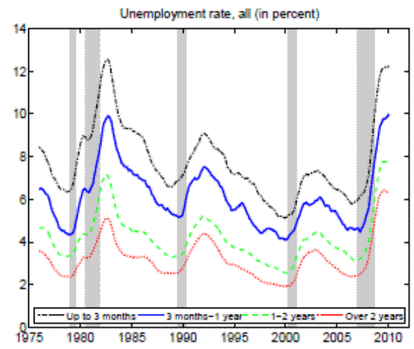 Figure 8a Data
Figure 8b. Unemployment rate by training requirements-Unemployment rate, high school graduates (in percent)
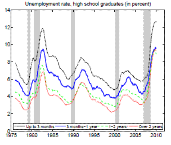 Figure 8b Data
Figure 8 depicts unemployment rates by training requirements for all individuals with 25 years of age and over (left panel) and for high school graduates with 25 years and over (right panel). Given the strong complementaries between education and job training (see the discussion in Section 2.4) it is not surprising to see that higher training requirements are associated with lower unemployment rates. What is more striking is that even after we control for education, for example by focusing on high school graduates as in the right panel of Figure 8, higher training levels remain to be related to more stable employment. Furthermore, even after we condition for education attainment, job training leads to empirically lower separation rates and similar job finding rates as shown in Figure 9. We view this novel empirical evidence, which shows that occupations with higher specific vocational training experience substantially lower unemployment rates, predominantly through lower separation rates, as an external validation of the theoretical mechanism advocated in this paper.
Figure 9a. Unemployment flow rates by training requirements, high school graduates-Outflow rate, high school graduates (in percent)
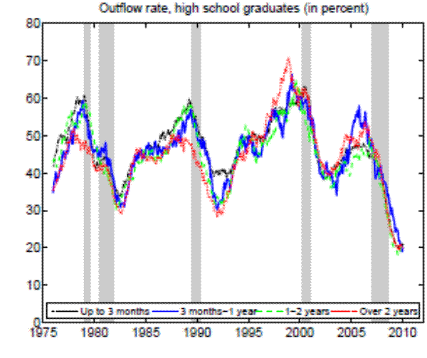 Figure 9a Data
Figure 9b. Unemployment flow rates by training requirements, high school graduates-Inflow rate, high school graduates (in percent)
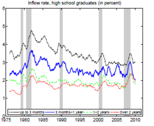 Figure 9b Data
8 Conclusions
In this paper we build a theoretical search and matching model with endogenous separations and initial on-the-job training. We use the model in order to explain differential unemployment properties across education groups. The model is parameterized by taking advantage of detailed micro evidence from the EOPP survey on the duration of on-the-job training and the productivity gap between new hires and incumbent workers across four education groups. In particular, the applied parameter values reflect strong complementarities between educational attainment and on-the-job training. The simulation results reveal that the model almost perfectly captures the empirical regularities across education groups on job finding rates, separation rates and unemployment rates, both in their first and second moments.
The analysis of this paper views training requirements as a technological constraint, inherent to the nature of the job. We believe that such a view is appropriate for the initial on-the-job training, for which we also have exact empirical measures that are used in the paper for the parameterization of the model. However, in reality firms provide training also to their workers in ongoing job relationships. To investigate such cases it would be worthwhile to endogenize the training decisions and examine interactions between training provision and job separations. Furthermore, one could take advantage of cross-country variation in labor market institutions that are likely to affect incentives for training provision. This could provide a new explanation for differential unemployment dynamics across countries, based on supportiveness of their respective labor market institutions to on-the-job training. We leave these extensions for future research.
References
Aguiar, M., and E. Hurst (2005): Consumption versus Expenditure, Journal of Political Economy, 113(5), 919-948.
Albrecht, J., and S. Vroman (2002): A Matching Model with Endogenous Skill Requirements, International Economic Review, 43(1), 283-305.
Altonji, J. G., and J. R. Spletzer (1991):Worker Characteristics, Job Characteristics, and the Receipt of On-the-Job Training, Industrial and Labor Relations Review, 45(1), 58-79.
Ashenfelter, O., and J. Ham (1979): Education, Unemployment, and Earnings, Journal of Political Economy, 87(5), S99-116.
Autor, D. H., F. Levy, and R. J. Murnane (2003): The Skill Content Of Recent Technological Change: An Empirical Exploration, The Quarterly Journal of Economics, 118(4), 1279-1333.
Barron, J. M., M. C. Berger, and D. A. Black (1997): How Well Do We Measure Training?, Journal of Labor Economics , 15(3), 507-28.
Bartel, A. P. (1995): Training, Wage Growth, and Job Performance: Evidence from a Company Database, Journal of Labor Economics, 13(3), 401-25.
Becker, G. S. (1964): Human Capital: A Theoretical and Empirical Analysis with Special Reference to Education. Columbia University Press, New York.
Bils, M., Y. Chang, and S.-B. Kim (2011): Worker Heterogeneity and Endogenous Separations in a Matching Model of Unemployment Fluctuations, American Economic Journal: Macroeconomics , 3(1), 128-54.
____(2012): Comparative advantage and unemployment, Journal of Monetary Economics, 59(2), 150-165.
Blanchard, O., and J. Gali (2010): Labor Markets and Monetary Policy: A New Keynesian Model with Unemployment, American Economic Journal: Macroeconomics, 2(2), 1-30.
Brown, J. N. (1989): Why Do Wages Increase with Tenure? On-the-Job Training and Life-Cycle Wage Growth Observed within Firms, American Economic Review, 79(5), 971-91.
Card, D., and A. B. Krueger (1994): Minimum Wages and Employment: A Case Study of the Fast-Food Industry in New Jersey and Pennsylvania, American Economic Review, 84(4), 772-93.
Costain, J., and M. Reiter (2008): Business Cycles, Unemployment Insurance, and the Calibration of Matching Models, Journal of Economic Dynamics and Control, 32(4), 1120-1155.
Couch, K. A., and D. W. Placzek (2010): Earnings Losses of Displaced Workers Revisited, American Economic Review, 100(1), 572-89.
Dolado, J. J., M. Jansen, and J. F. Jimeno (2009): On-the-Job Search in a Matching Model with Heterogeneous Jobs and Workers, Economic Journal, 119(534), 200-228.
Dube, A., T. W. Lester, and M. Reich (2010): Minimum Wage Effects Across State Borders: Estimates Using Contiguous Counties, The Review of Economics and Statistics, 92(4), 945-964.
Elsby, M. W. L., B. Hobijn, and A. Sahin (2010): The Labor Market in the Great Recession, Brookings Papers on Economic Activity, Spring 2010, 1-48.
Elsby, M. W. L., R. Michaels, and G. Solon (2009): The Ins and Outs of Cyclical Unemployment, American Economic Journal: Macroeconomics, 1(1), 84-110.
Fujita, S., and G. Ramey (2009): The Cyclicality of Separation and Job Finding Rates, International Economic Review, 50(2), 415-430.
____(2012): Exogenous versus Endogenous Separation, American Economic Journal: Macroeconomics, 4(4), 68-93.
Gautier, P. A. (2002): Unemployment and Search Externalities in a Model with Heterogeneous Jobs and Workers, Economica, 69(273), 21-40.
Gomes, P. (2012): Labour market flows: Facts from the United Kingdom, Labour Economics, 19(2), 165-175.
Gomme, P., R. Rogerson, P. Rupert, and R. Wright (2005): The Business Cycle and the Life Cycle, in NBER Macroeconomics Annual 2004, Volume 19, NBER Chapters, pp. 415-592. National Bureau of Economic Research.
Gonzalez, F. M., and S. Shi (2010): ''An Equilibrium Theory of Learning, Search, and Wages, Econometrica, 78(2), 509-537.
Hagedorn, M., and I. Manovskii (2008): The Cyclical Behavior of Equilibrium Unemployment and Vacancies Revisited, American Economic Review, 98(4), 1692-1706.
Hall, R. E., and P. R. Milgrom (2008): The Limited Influence of Unemployment on the Wage Bargain, American Economic Review, 98(4), 1653-74.
Hosios, A. J. (1990): On the Efficiency of Matching and Related Models of Search and Unemployment, Review of Economic Studies, 57(2), 279-98.
Jacobson, L. S., R. J. LaLonde, and D. G. Sullivan (1993): Earnings Losses of Displaced Workers, American Economic Review, 83(4), 685-709.
Jaeger, D. A. (1997): Reconciling the Old and New Census Bureau Education Questions: Recommendations for Researchers, Journal of Business & Economic Statistics, 15(3), 300-09.
Jovanovic, B. (1979): Firm-specific Capital and Turnover, Journal of Political Economy, 87(6), 1246-60.
Kambourov, G., and I. Manovskii (2008): Rising Occupational And Industry Mobility In The United States: 1968-97, International Economic Review, 49(1), 41-79.
____(2009): Occupational Mobility and Wage Inequality, Review of Economic Studies , 76(2), 731-759.
Kopecky, K., and R. Suen (2010): Finite State Markov-chain Approximations to Highly Persistent Processes, Review of Economic Dynamics, 13(3), 701-714.
Krusell, P., T. Mukoyama, and A. Sahin (2010): Labour-Market Matching with Precautionary Savings and Aggregate Fluctuations, Review of Economic Studies, 77(4), 1477-1507.
Kydland, F. E. (1984): Labor-force heterogeneity and the business cycle, Carnegie Rochester Conference Series on Public Policy, 21(1), 173-208.
Lemieux, T. (2006): Increasing Residual Wage Inequality: Composition Effects, Noisy Data, or Rising Demand for Skill?, American Economic Review, 96(3), 461-498.
Lillard, L. A., and H. W. Tan (1986): Private Sector Training: Who Gets It and What Are Its Effects?, Discussion Paper R-3331, Rand Corporation.
Ljungqvist, L., and T. J. Sargent (1998): The European Unemployment Dilemma, Journal of Political Economy, 106(3), 514-550.
____(2007): Understanding European Unemployment with Matching and Search-Island Models, Journal of Monetary Economics, 54(8), 2139-2179.
Lynch, L. M. (1991): The Role of Off-the-Job vs. On-the-Job Training for the Mobility of Women Workers, American Economic Review, 81(2), 151-56.
____(1992): Private-Sector Training and the Earnings of Young Workers, American Economic Review, 82(1), 299-312.
Meyer, B. D. (1990): Unemployment Insurance and Unemployment Spells, Econometrica, 58(4), 757-82.
Mincer, J. (1991): Education and Unemployment, NBER Working Paper 3838.
Moffitt, R. (1985): Unemployment Insurance and the Distribution of Unemployment Spells, Journal of Econometrics, 28(1), 85-101.
Mortensen, D. T., and E. Nagypal (2007): More on Unemployment and Vacancy Fluctuations, Review of Economic Dynamics, 10(3), 327-347.
Mortensen, D. T., and C. A. Pissarides (1994): Job Creation and Job Destruction in the Theory of Unemployment, Review of Economic Studies, 61(3), 397-415.
____(1999): Unemployment Responses to Skill-Biased Technology Shocks: The Role of Labour Market Policy, Economic Journal, 109(455), 242-65.
Nickell, S. (1979): Education and Lifetime Patterns of Unemployment, Journal of Political Economy, 87(5), S117-31.
Oi, W. Y. (1962): Labor as a Quasi-Fixed Factor, Journal of Political Economy, 70(6), 538-555.
Petrongolo, B., and C. A. Pissarides (2001): Looking into the Black Box: A Survey of the Matching Function, Journal of Economic Literature, 39(2), 390-431.
Pissarides, C. A. (2000): Equilibrium Unemployment Theory . MIT Press, Cambridge, MA.
____(2009): The Unemployment Volatility Puzzle: Is Wage Stickiness the Answer?, Econometrica, 77(5), 1339-1369.
Pries, M. J. (2008): Worker Heterogeneity and Labor Market Volatility in Matching Models, Review of Economic Dynamics, 11(3), 664-678.
Rouwenhorst, K. G. (1995): Asset Pricing Implications of Equilibrium Business Cycle Models, in frontiers of Business Cycle Research, ed. by T. F. Cooley, pp. 294-330. Princeton University Press, Princeton.
Shimer, R. (2005): The Cyclical Behavior of Equilibrium Unemployment and Vacancies, American Economic Review, 95(1), 25-49.
____(2009): Labor Markets and Business Cycles. Princeton University Press, Princeton.
____(2012): Reassessing the Ins and Outs of Unemployment, Review of Economic Dynamics , 15(2), 127-148.
Silva, J. I., and M. Toledo (2009): Labor Turnover Costs and The Cyclical Behavior of Vacancies and Unemployment, Macroeconomic Dynamics, 13(S1), 76-96.
Topel, R. H. (1991): Specific Capital, Mobility, and Wages: Wages Rise with Job Seniority, Journal of Political Economy, 99(1), 145-76.
van Ours, J. C., and G. Ridder (1993): Vacancy Durations: Search or Selection?, Oxford Bulletin of Economics and Statistics, 55(2), 187-98.
A.1 Current Population Survey
In order to construct unemployment rates, inflows, and outflows by education group we use the Current Population Survey (CPS) basic monthly data files from January 1976 until December 2010, accessed through http://www.nber.org/cps/. From these data we obtain the total number of employed, the total number of unemployed and the number of short-term (less than 5 weeks) unemployed for each education group. The calculation of unemployment rates follows the usual definition (unemployed/labor force).
In January 1992 the U.S. Census Bureau modified the CPS question on educational attainment. In particular, before 1992 the question was about the highest grade attended and completed (years of education), whereas after that the question has been about the highest degree received. We broadly follow suggestions by Jaeger (1997) on categorical recoding schemes for old and new education questions. Our education groups consist of: i) less than high school (0-12 years uncompleted according to the old question; at most 12th grade, no diploma according to the new question); ii) high school graduates (12 years completed; high school graduates); iii) some college (13-16 years uncompleted; some college, associate's degrees); iv) college graduates (16 years completed and more; bachelor's, master's, professional school and doctoral degrees).
Moreover, due to the January 1994 CPS redesign there is a discontinuity in the short-term unemployment series.40 More precisely, from 1994 onwards the CPS does not ask about unemployment duration a worker who is unemployed in consecutive months, but instead his duration is calculated as the sum of unemployment duration in the previous month plus the intervening number of weeks. Nevertheless, workers in the incoming rotation groups (1st and 5th) are always asked about unemployment duration, even after 1994. This allows to calculate the ratio of the short-term unemployed share for the 1st and 5th rotation groups relative to the short-term unemployed share in the full sample. One can then multiply the short-term unemployment series after 1994 by this ratio. Since the ratio turns out to be quite volatile over time, we follow the suggestion by Elsby, Michaels, and Solon (2009) and multiply the series by the average value of the ratio for the period February 1994 - December 2010. We apply this correction for each education group separately, although the ratios are very similar across groups. More precisely, the ratio equals to 1.14 (1.17 when limiting the sample to 16 years of age and over) for high school dropouts, 1.14 (1.16) for high school graduates, 1.14 (1.14) for people with some college, 1.13 (1.15) for college graduates, and 1.14 (1.16) for aggregate numbers. Note that the aggregate number for the whole sample is very close to the one calculated by Elsby, Michaels, and Solon (2009), who find an average ratio of 1.15 for the period February 1994 - January 2005.
Next, we seasonally adjust the series using the X-12-ARIMA seasonal adjustment program (version 0.3), provided by the U.S. Census Bureau. Then we compute the monthly outflow and inflow rates. The outflow rate can be obtained from the equation describing the law of motion for unemployment:
![]() , where
, where ![]() denotes unemployed,
denotes unemployed, ![]() short-term unemployed and
short-term unemployed and ![]() the monthly outflow probability. The latter is hence
given by
the monthly outflow probability. The latter is hence
given by
![]() , with the outflow hazard rate being
, with the outflow hazard rate being
![]() . To calculate inflow rates, we use the continuous-time correction for time aggregation bias from Shimer (2012), which takes into account that some workers who
become unemployed, manage to find a new job before the next CPS survey arrives.
. To calculate inflow rates, we use the continuous-time correction for time aggregation bias from Shimer (2012), which takes into account that some workers who
become unemployed, manage to find a new job before the next CPS survey arrives.
A.2 Employment Opportunity Pilot Project Survey
The 1982 Employment Opportunity Pilot Project (EOPP) was a survey of employers in the United States conducted between February and June 1982. The survey had three parts. The first part collected information on general hiring practices, the second part asked the employer about the last hired worker and the last part dealt with government programs. We focus only on the central part of the survey, given that it provides specific information about the relationship between education and the degree of on-the-job training. In particular, employers were asked to think about the last new employee the company hired prior to August 1981 regardless of whether that person was still employed by the company at the time of the interview. A series of specific questions were asked about the training received by the new employee during the first three months in the company.
The main advantage of the 1982 EOPP survey is that it includes both measures of formal and informal training. Nevertheless, some drawbacks of the 1982 EOPP survey need to be mentioned as well. First, the sample of employers interviewed is not representative. In particular, the sample was intentionally designed to overrepresent low-paid jobs. Second, given that questions were related to the last hire in the company, the sample also most likely overrepresents workers with higher turnover rates. Finally, although the survey has been widely used to study several aspects of on-the-job training, it is becoming outdated and thus perhaps less relevant. To overcome some of these concerns, we use the data from the 1979 National Longitudinal Survey of Youth as a supplementary data source on (formal) on-the-job training.
A.3 National Longitudinal Survey of Youth
The 1979 National Longitudinal Survey of Youth (NLSY) contains a nationally representative sample of 12,686 young men and women who were 14-22 years old when they were first surveyed in 1979. These individuals were interviewed annually through 1994 and are currently interviewed on a biennial basis. The measure of training incidence used in the text comes from the following question in the survey: "Since [date of the last interview], did you attend any training program or any on-the-job training designed to improve job skills, help people find a job, or learn a new job?". Notice that this question has a 1-year reference period in 1989-1994, while it has a 2-year reference period in 1988 and from 1996 onwards. As mentioned in the text, the analysis of the NLSY data supports the main empirical findings from the 1982 EOPP data regarding the existence of on-the-job training differences across education groups.
B.1 Unemployment Rates by Education
Table 11 shows results from estimated regression equations, where the probability of being unemployed is being regressed on the standard set of controls. These results show that education remains an important predictor of the probability of being unemployed, even when controlling for demographic characteristics, industry, occupation, and including time dummies.
| (1) | (2) | (3) | (4) | (5) | (6) | |
| Less Than High School | 0.0986*** | 0.0749*** | 0.0764*** | 0.0487*** | 0.0402*** | 0.0372*** |
| Less Than High School (std. errors) | (0.0005) | (0.0005) | (0.0005) | (0.0005) | (0.0005) | (0.0005) |
| High School | 0.0430*** | 0.0327*** | 0.0334*** | 0.0233*** | 0.0165*** | 0.0152*** |
| High School (std. errors) | (0.0003) | (0.0003) | (0.0003) | (0.0003) | (0.0003) | (0.0003) |
| Some College | 0.0253*** | 0.0137*** | 0.0140*** | 0.0108*** | 0.0068*** | 0.0061*** |
| Some College (std. errors) | (0.0002) | (0.0002) | (0.0002) | (0.0002) | (0.0003) | (0.0003) |
| Individual controls | yes | yes | yes | yes | yes | |
| Time dummies | yes | yes | yes | yes | ||
| Industry controls | yes | yes | ||||
| Occupation controls | yes | yes | ||||
| Observations | 6,701,078 | 6,701,078 | 6,701,078 | 6,670,335 | 6,670,335 | 6,670,335 |
| R-squared | 0.015 | 0.0321 | 0.0385 | 0.0367 | 0.0355 | 0.0389 |
Figure 10a. U.S. unemployment rates, educational attainment and age-U.S. unemployment rates
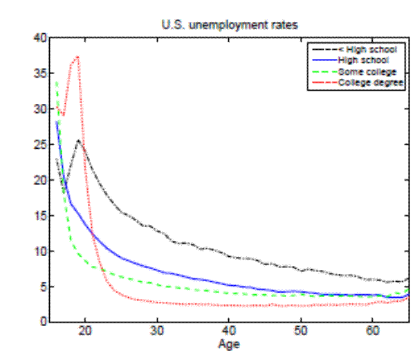 Figure 10a Data
Notes: The sample period is 2003:01-2010:12. All variables are constructed from CPS microdata.
Figure 12a. Unemployment duration shares by education groups-Employment Unemployment transition rate
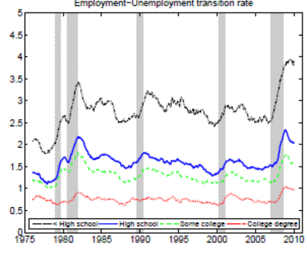 Figure 12a Data
Figure 12b. Unemployment duration shares by education groups-Employment Inactivity transition rate
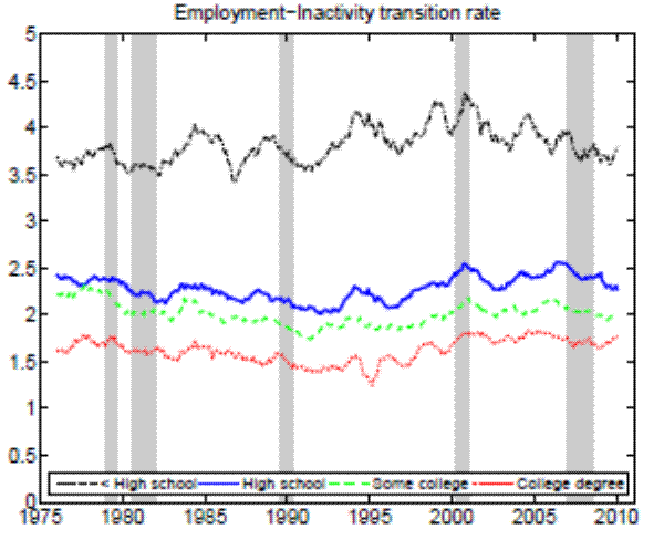 Figure 12b Data
Figure 12c. Unemployment duration shares by education groups-Unemployment Employment transition rate
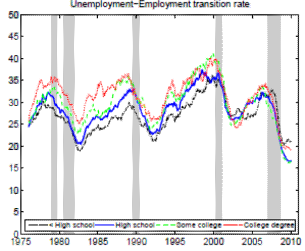 Figure 12c Data
Figure 12d. Unemployment duration shares by education groups-Unemployment Inactivity transition rate
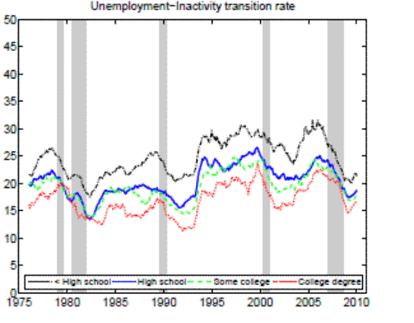 Figure 12d Data
Figure 12e. Unemployment duration shares by education groups-Inactivity Employment transition rate
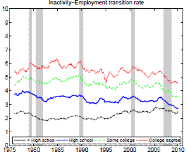 Figure 12e Data
Figure 12f. Unemployment duration shares by education groups-Inactivity Unemployment transition rate
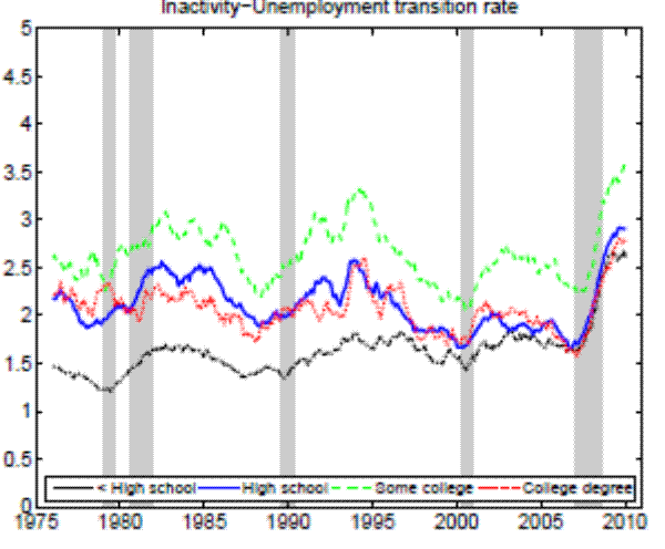 Figure 12f Data
Figure 13a. Counterfactual unemployment rates (25+ years of age)- The role of EmploymentUnemployment transition rate
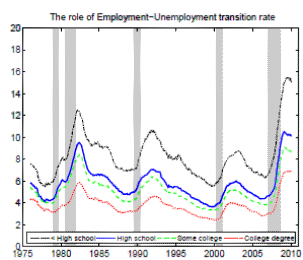 Figure 13a Data
Figure 13b. Counterfactual unemployment rates (25+ years of age)- The role of Employment Inactivity transition rate
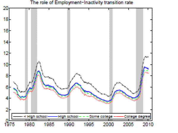 Figure 13b Data
Figure 13c. Counterfactual unemployment rates (25+ years of age)- The role of Unemployment Employment transition rate
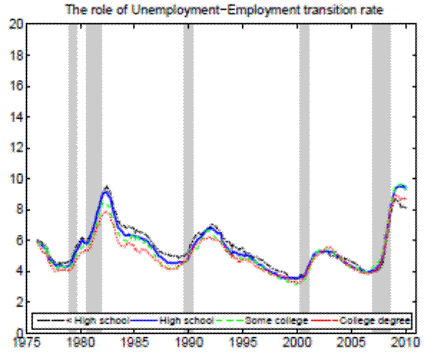 Figure 13c Data
Figure 13d. Counterfactual unemployment rates (25+ years of age)- The role of Unemployment Inactivity transition rate
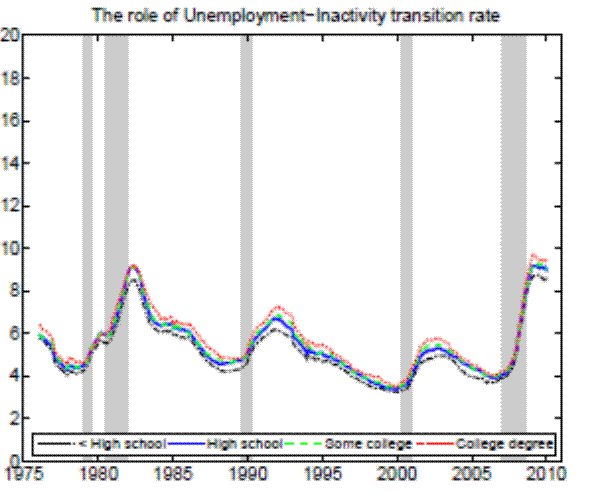 Figure 13d Data
Figure 13e. Counterfactual unemployment rates (25+ years of age)- The role of Inactivity Employment transition rate
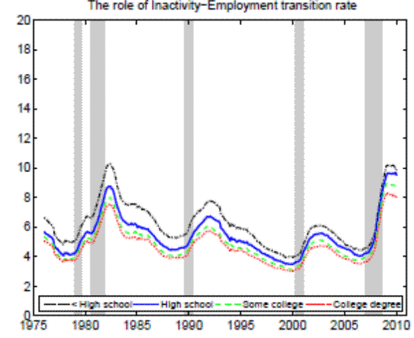 Figure 13e Data
Figure 13f. Counterfactual unemployment rates (25+ years of age)- The role of InactivityUnemployment transition rate
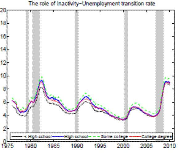 Figure 13f Data
Figure 15a. Counterfactual unemployment rates (16+ years of age)-The role of outflow rate
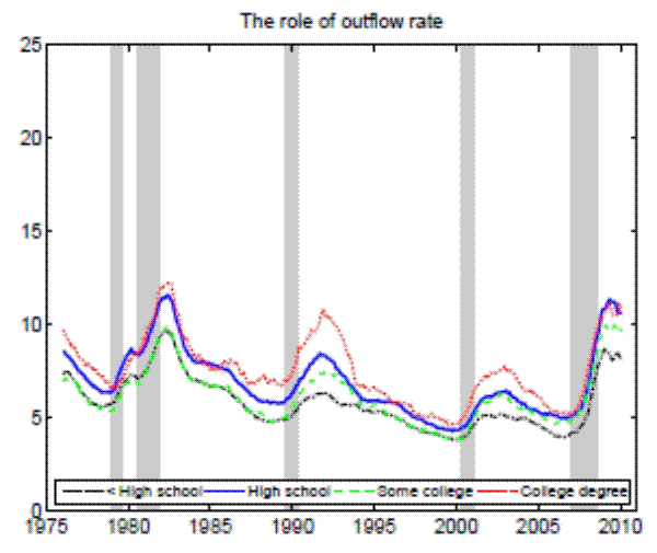 Figure 15a Data
Figure 15b. Counterfactual unemployment rates (16+ years of age)-The role of inflow rate
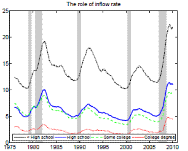 Figure 15b Data
C.1.1 The Constrained-Efficient Allocation
In order to investigate the efficiency properties of the model, we derive the constrained-efficient allocation by solving the problem of a benevolent social planner. Given the assumption on risk neutrality of agents in the model, we naturally abstract from distributive inefficiency and instead
examine inefficiency arising exclusively due to search externalities. The social planner takes as given the search frictions and the training requirements. We abstract from aggregate productivity shocks and assume that idiosyncratic shocks are being drawn in each period from a continuous
distribution ![]() , which simplifies some of the derivations.
, which simplifies some of the derivations.
The benevolent social problem chooses ![]() ,
,
![]() and
and
![]() in order to maximize the utility of the representative worker by solving the following Bellman equation for each submarket
in order to maximize the utility of the representative worker by solving the following Bellman equation for each submarket ![]() :
:
 |
 |
|
 |
with
 |
||
 |
subject to the following laws of motion for employment:
![\displaystyle \left[ (1-\delta)(1-\phi_h) \int_{\tilde{a}^T}^{\infty} n^T(a) dG(a) + \gamma \theta^{1-\alpha} \left( 1 - n \right) \right] G(x),](img194.gif) |
||
![\displaystyle \left[ (1-\delta) \int_{\tilde{a}^S}^{\infty} n^S(a) dG(a) + (1-\delta) \phi_h \int_{\tilde{a}^T}^{\infty} n^T(a) dG(a) \right] G(x).](img196.gif) |
Note that
The first order conditions are:
 |
||
 |
||
 |
||
 |
The envelope conditions are:
 |
 |
|
 |
||
 |
||
 |
 |
|
 |
||
 |
After some rearrangements, the following optimal job creation condition can be obtained:
Similarly, the optimal job destruction conditions are given by:
C.1.2 Decentralized Allocation
Again, we abstract from aggregate productivity shocks and assume that idiosyncratic shocks are being drawn in each period from a continuous distribution ![]() . The main equilibrium
conditions are:
. The main equilibrium
conditions are:
 |
||
 |
||
 |
||
 |
||
 |
||
 |
Notice that we can write:
 |
 |
So, we have the following job creation condition:
The job destruction conditions can be derived as:
By comparing the constrained-efficient equilibrium conditions (13)-(15) with the decentralized equilibrium conditions (16)-(18) it follows that the decentralized allocation replicates the constrained-efficient
allocation when
![]() , reflecting the standard Hosios condition.
, reflecting the standard Hosios condition.
C.1.3 Worker's bargaining power and job destruction - analytical results
Subtracting
![]() from
from
![]() and
and
![]() from
from
![]() we get:
we get:
Using the above in the job creation condition gives:


 |
 |
|
 |
Making an analogous substitutions and taking derivative of the job destruction condition for skilled workers with respect to
 |
 |
Combining the above and rearranging gives:
 |
 |
|
 |
 |
where:
 |
||
 |
||
 |
Note that
As we move away from the Hosios efficiency condition, we have:

C.1.4 Worker's bargaining power and job destruction - numerical results
Figure 16 illustrates how different values of bargaining power affect both job destruction margins under our baseline calibration. Note that in this numerical exercise we allow for aggregate productivity shocks and some persistence in idiosyncratic productivity shocks.
Notes: Results from solving the model for different values of workers bar gaining power, keeping the rest of parameters constant at the aggregate level.
C.2 Computational Strategy
In order to solve the model numerically, we discretize the state space. In particular, the aggregate shock ![]() is approximated with a Markov chain of 11 equally spaced gridpoints, whereas
the idiosyncratic shock
is approximated with a Markov chain of 11 equally spaced gridpoints, whereas
the idiosyncratic shock ![]() is approximated by a discrete lognormal distribution with its support having 700 equally spaced gridpoints. We truncate the lognormal distribution at 0.01 percent
and 99.99 percent and then normalize probabilities so that they sum up to one. The solution algorithm consists of value function iteration until convergence. The final model's solution consists of equilibrium labor market tightness
is approximated by a discrete lognormal distribution with its support having 700 equally spaced gridpoints. We truncate the lognormal distribution at 0.01 percent
and 99.99 percent and then normalize probabilities so that they sum up to one. The solution algorithm consists of value function iteration until convergence. The final model's solution consists of equilibrium labor market tightness
![]() and reservation productivities
and reservation productivities
![]() and
and
![]() . This solution is then used to simulate the model.
. This solution is then used to simulate the model.
Appendix D. Sensitivity Analysis of the Quantitative Results
Here we provide the sensitivity analysis of our main quantitative results from Section 5 of the paper where differences in unemployment dynamics by education are explained by differences in on-the-job training. We perform two types of robustness checks for our quantitative results. First, we explore the role of parameter for the flow value when being unemployed, both regarding its overall level and differences across education groups. Second, we consider different specification for the flow vacancy posting costs. Simulations results for all robustness checks are summarized in Table 12.
| Less than high school | 8.96 | 46.85 | 4.45 |
| High school | 5.45 | 45.02 | 2.48 |
| Some college | 4.44 | 46.34 | 2.05 |
| College degree | 2.56 | 42.80 | 1.09 |
Notes: Data moments are quarterly averages of monthly seasonally-adjusted data constructed from CPS microdata. The sample period is 1976:01 - 2010:12. Statistics for the model are means across 100 simulations.
| Less than high school | 2.35 | 0.163 | 0.71 | 7.26 | 45.32 | 3.52 |
| High school | 2.78 | 0.181 | 0.71 | 5.89 | 45.06 | 2.80 |
| Some college | 3.67 | 0.227 | 0.71 | 2.98 | 45.51 | 1.38 |
| College degree | 4.19 | 0.240 | 0.71 | 2.27 | 45.75 | 1.06 |
Notes: Data moments are quarterly averages of monthly seasonally-adjusted data constructed from CPS microdata. The sample period is 1976:01 - 2010:12. Statistics for the model are means across 100 simulations.
| Less than high school | 2.35 | 0.163 | 0.82 | 39.98 | 17.29 | 10.98 |
| High school | 2.78 | 0.181 | 0.82 | 12.16 | 34.24 | 4.52 |
| Some college | 3.67 | 0.227 | 0.82 | 1.91 | 54.79 | 1.05 |
| College degree | 4.19 | 0.240 | 0.82 | 0.98 | 80.05 | 0.79 |
Notes: Data moments are quarterly averages of monthly seasonally-adjusted data constructed from CPS microdata. The sample period is 1976:01 - 2010:12. Statistics for the model are means across 100 simulations.
| Less than high school | 2.35 | 0.163 | 0.090 | 7.67 | 45.89 | 3.73 |
| High school | 2.78 | 0.181 | 0.104 | 5.93 | 44.77 | 2.74 |
| Some college | 3.67 | 0.227 | 0.121 | 2.87 | 44.12 | 1.27 |
| College degree | 4.19 | 0.240 | 0.128 | 2.47 | 46.60 | 1.15 |
Notes: Data moments are quarterly averages of monthly seasonally-adjusted data constructed from CPS microdata. The sample period is 1976:01 - 2010:12. Statistics for the model are means across 100 simulations.
| Less than high school | 2.35 | 0.163 | 0.106 | 6.79 | 43.69 | 3.11 |
| High school | 2.78 | 0.181 | 0.106 | 5.67 | 44.82 | 2.63 |
| Some college | 3.67 | 0.227 | 0.106 | 3.12 | 46.19 | 1.45 |
| College degree | 4.19 | 0.240 | 0.106 | 2.76 | 49.12 | 1.35 |
Notes: Data moments are quarterly averages of monthly seasonally-adjusted data constructed from CPS microdata. The sample period is 1976:01 - 2010:12. Statistics for the model are means across 100 simulations.
| Less than high school | 2.35 | 0.163 | 0.212 | 7.79 | 45.67 | 3.78 |
| High school | 2.78 | 0.181 | 0.212 | 6.14 | 45.37 | 2.89 |
| Some college | 3.67 | 0.227 | 0.212 | 2.99 | 45.13 | 1.35 |
| College degree | 4.19 | 0.240 | 0.212 | 2.34 | 45.32 | 1.06 |
D.1.1 Value of being unemployed - overall level
Here we set ![]() as in Hall and Milgrom (2008) and Pissarides (2009). Consistent with our calibration procedure we adjust the matching efficiency parameter to
as in Hall and Milgrom (2008) and Pissarides (2009). Consistent with our calibration procedure we adjust the matching efficiency parameter to
![]() in order to target the average job finding rate and we adjust the standard deviation of idiosyncratic productivity shocks to
in order to target the average job finding rate and we adjust the standard deviation of idiosyncratic productivity shocks to
![]() in order to hit the average separation rate. The rest of the numerical exercise follows the same steps as in Section 5, including the same
parameter values for on-the-job training by education. The simulation results are provided in Panel B of Table 12 and are to be compared with results in Table 7. Note that with
in order to hit the average separation rate. The rest of the numerical exercise follows the same steps as in Section 5, including the same
parameter values for on-the-job training by education. The simulation results are provided in Panel B of Table 12 and are to be compared with results in Table 7. Note that with ![]() our results remain basically unchanged with respect to our baseline calibration. The unemployment ratio between high school dropouts and college graduates was 3.4 under our baseline calibration, whereas with
our results remain basically unchanged with respect to our baseline calibration. The unemployment ratio between high school dropouts and college graduates was 3.4 under our baseline calibration, whereas with ![]() it is 3.2 (to be compared with 3.5 in the data). The only noticeable difference concerns the volatility results. In particular, now the aggregate volatilities of labor market variables are lower by half - the unemployment
volatility puzzle becomes more evident and this is also the only reason that we chose a somewhat higher
it is 3.2 (to be compared with 3.5 in the data). The only noticeable difference concerns the volatility results. In particular, now the aggregate volatilities of labor market variables are lower by half - the unemployment
volatility puzzle becomes more evident and this is also the only reason that we chose a somewhat higher ![]() in our baseline calibration. Nevertheless, also with
in our baseline calibration. Nevertheless, also with ![]() the relative differences in volatilities across education groups remain present; the unemployment volatility ratio between high school dropouts and college graduates was 3.7 under our baseline calibration, whereas
now it is 3.2, the same as in the data.41
the relative differences in volatilities across education groups remain present; the unemployment volatility ratio between high school dropouts and college graduates was 3.7 under our baseline calibration, whereas
now it is 3.2, the same as in the data.41
D.1.2 Constant value of being unemployed across education groups
Below we present a robustness check when we deviate from the proportionality assumption and we keep ![]() constant at 0.82 for all four education groups. As the result of Proposition
1 does not apply anymore, we need to parameterize differences in the market labor productivity across education groups,
constant at 0.82 for all four education groups. As the result of Proposition
1 does not apply anymore, we need to parameterize differences in the market labor productivity across education groups, ![]() . We do so by taking advantage of the
1982 EOPP data, which contain information on hourly wage. Hourly wage data allow us to impute productivity differences
. We do so by taking advantage of the
1982 EOPP data, which contain information on hourly wage. Hourly wage data allow us to impute productivity differences ![]() , which are reported in Table 13. The
parametrized productivity differences are broadly in line with estimates obtained by the literature on returns to schooling.42 After simulating the model,
we can express the flow value of being unemployed relative to the effective productivity. The obtained values for the effective flow value of being unemployed are 88.7 percent for high school dropouts, 85.0 percent for high school graduates, 77.2 percent for people with some college, and 61.2
percent for college graduates. In short, the size of match surplus is now increasing with education.
, which are reported in Table 13. The
parametrized productivity differences are broadly in line with estimates obtained by the literature on returns to schooling.42 After simulating the model,
we can express the flow value of being unemployed relative to the effective productivity. The obtained values for the effective flow value of being unemployed are 88.7 percent for high school dropouts, 85.0 percent for high school graduates, 77.2 percent for people with some college, and 61.2
percent for college graduates. In short, the size of match surplus is now increasing with education.
| Hourly Wage | Implied Productivity |
|
| Less than high school | 5.60 | 0.84 |
| High school | 6.21 | 0.93 |
| Some college | 7.07 | 1.06 |
| College degree | 8.96 | 1.35 |
| All individuals | 6.65 | 1 |
Notes: Productivity differences, ![]() , are imputed from the hourly wage data in the 1982 EOPP survey. We normalize the average productivity in the economy to
1.
, are imputed from the hourly wage data in the 1982 EOPP survey. We normalize the average productivity in the economy to
1.
Panel C of Table 12 presents the simulation results. In particular, we solve and simulate the model for each education group, by using the corresponding training parameters (![]() and
and ![]() ), the constant flow value of being unemployed (
), the constant flow value of being unemployed (![]() ) and productivity parameters (
) and productivity parameters (![]() ) for each education group, while keeping the rest of parameters constant at the aggregate level. It turns out that when we deviate
from the proportionality assumption
) for each education group, while keeping the rest of parameters constant at the aggregate level. It turns out that when we deviate
from the proportionality assumption ![]() , the model yields highly counterfactual predictions. In particular, the job finding rate for college graduates is now more than four times higher
than the one for high school dropouts, whereas in the data they are practically identical. Additionally, the simulation results for college graduates suffer from extreme unemployment volatility puzzle, as their unemployment rate remains virtually constant over the business cycle.43 The simulation results with constant absolute flow value of being unemployed also severely overpredict differences in unemployment and separation rates across
education groups.
, the model yields highly counterfactual predictions. In particular, the job finding rate for college graduates is now more than four times higher
than the one for high school dropouts, whereas in the data they are practically identical. Additionally, the simulation results for college graduates suffer from extreme unemployment volatility puzzle, as their unemployment rate remains virtually constant over the business cycle.43 The simulation results with constant absolute flow value of being unemployed also severely overpredict differences in unemployment and separation rates across
education groups.
D.2 Vacancy posting costs
Next, we examine the quantitative implications of the model when considering different assumptions regarding the vacancy costs. In particular, three robustness exercises will be carried out. The first one considers the actual data from the 1982 EOPP survey to infer the vacancy posting cost for each education group. The second exercise considers the same absolute value of vacancy posting costs for all education groups. In the last exercise we double the vacancy posting cost used in our baseline calibration.
D.2.1 Actual vacancy posting costs from the 1982 EOPP survey
The 1982 EOPP data contain evidence on vacancy duration and recruitment costs. Table 14 summarizes these data across education groups.44 The column denoted "![]() " presents vacancy posting costs expressed in terms of output for each corresponding education group. As it can be seen, the vacancy
posting costs across education groups remain close to the aggregate level, which is consistent with our assumption
" presents vacancy posting costs expressed in terms of output for each corresponding education group. As it can be seen, the vacancy
posting costs across education groups remain close to the aggregate level, which is consistent with our assumption ![]() . The calculated vacancy posting costs exhibit very little variation
across education groups due to two counteracting effects in the data. On the one hand, recruitment costs in terms of hours spent are indeed much higher for more educated workers. On the other hand, the 1982 EOPP data also show higher vacancy duration for more educated workers. Note that the latter
observation is inconsistent with the empirical evidence of similar job finding rates across education groups, under the assumption of identical matching efficiency across groups. However, longer vacancy duration for more educated workers might not be due to lower vacancy meeting probability, but
might simply reflect that the recruitment process itself is longer for this group of workers, perhaps for administrative reasons. In this respect, van Ours and Ridder (1993) provide evidence that the vacancy duration consists of an application period, during which applicants arrive, and a selection
period, during which a new employee is chosen from the pool of applicants. They conclude that the mean selection period increases with the required level of education, while required education has no effect on the applicant arrival rate. The applicant arrival rate is arguably the empirical
counterpart for the vacancy meeting probability of a theoretical search model. Finally note that in the calibration of search and matching models, vacancy duration is merely a normalization, as its changes can be undone by adjusting the flow vacancy posting cost and matching efficiency.45
. The calculated vacancy posting costs exhibit very little variation
across education groups due to two counteracting effects in the data. On the one hand, recruitment costs in terms of hours spent are indeed much higher for more educated workers. On the other hand, the 1982 EOPP data also show higher vacancy duration for more educated workers. Note that the latter
observation is inconsistent with the empirical evidence of similar job finding rates across education groups, under the assumption of identical matching efficiency across groups. However, longer vacancy duration for more educated workers might not be due to lower vacancy meeting probability, but
might simply reflect that the recruitment process itself is longer for this group of workers, perhaps for administrative reasons. In this respect, van Ours and Ridder (1993) provide evidence that the vacancy duration consists of an application period, during which applicants arrive, and a selection
period, during which a new employee is chosen from the pool of applicants. They conclude that the mean selection period increases with the required level of education, while required education has no effect on the applicant arrival rate. The applicant arrival rate is arguably the empirical
counterpart for the vacancy meeting probability of a theoretical search model. Finally note that in the calibration of search and matching models, vacancy duration is merely a normalization, as its changes can be undone by adjusting the flow vacancy posting cost and matching efficiency.45
| Vacancy duration (in days) | Recruitment costs (in hours) | Wage | ||||
| Less than high school | 12.2 | 7.8 | 0.107 | 5.60 | 0.84 | 0.090 |
| High school | 14.2 | 9.4 | 0.111 | 6.21 | 0.93 | 0.104 |
| Some college | 20.2 | 13.9 | 0.114 | 7.07 | 1.06 | 0.121 |
| College degree | 33.8 | 19.3 | 0.095 | 8.96 | 1.35 | 0.128 |
| All individuals | 17.8 | 11.3 | 0.106 | 6.65 | 1 | 0.106 |
Since some differences in flow vacancy posting costs are present across education groups, we use the exact information on these costs to parameterize our model as a robustnesses check. In order to do that, we express all flow vacancy posting costs in terms of aggregate output and again
parameterize differences in productivity across education groups. The column denoted "Wage" corresponds to the 1982 EOPP hourly wage, from which we impute productivity differences ![]() . The
last column of Table 14 gives us the parameter values to use in the simulations for each education group. We solve and simulate the model for each education group, by using the corresponding training parameters (
. The
last column of Table 14 gives us the parameter values to use in the simulations for each education group. We solve and simulate the model for each education group, by using the corresponding training parameters (![]() and
and ![]() ), actual vacancy posting cost (
), actual vacancy posting cost (![]() ) and productivity parameters (
) and productivity parameters (![]() ) for each education group, while keeping the rest of parameters constant at the aggregate level.46 Panel D of Table 12 reports the simulation results and, as we can see, they do not differ much from our simulation results in Section 5.
Therefore, our simulation results are robust when considering the actual vacancy posting costs from the 1982 EOPP survey.
) for each education group, while keeping the rest of parameters constant at the aggregate level.46 Panel D of Table 12 reports the simulation results and, as we can see, they do not differ much from our simulation results in Section 5.
Therefore, our simulation results are robust when considering the actual vacancy posting costs from the 1982 EOPP survey.
D.2.2 Constant vacancy posting costs across education groups
Panel E of Table 12 reports simulation results when we set ![]() for all four education groups, hence deviating from the assumption of proportionality in vacancy
posting costs. We solve and simulate the model for each education group, by using the corresponding training parameters (
for all four education groups, hence deviating from the assumption of proportionality in vacancy
posting costs. We solve and simulate the model for each education group, by using the corresponding training parameters (![]() and
and ![]() ), vacancy posting cost (
), vacancy posting cost (![]() ) and productivity parameters (
) and productivity parameters (![]() ) for each education group, while keeping the rest of parameters constant at the aggregate level. Note that this exercise presents an extreme case, in the sense that the vacancy posting cost is the same in absolute value across education groups,
implying that in terms of output it is decreasing with education. The simulation results remain virtually unchanged, implying again that the parameterization of
) for each education group, while keeping the rest of parameters constant at the aggregate level. Note that this exercise presents an extreme case, in the sense that the vacancy posting cost is the same in absolute value across education groups,
implying that in terms of output it is decreasing with education. The simulation results remain virtually unchanged, implying again that the parameterization of ![]() is not crucial for our
conclusions.
is not crucial for our
conclusions.
D.2.3 Doubling vacancy posting costs
In the last robustness exercise with respect to the vacancy posting cost we double the value used in our baseline calibration, increasing ![]() from 0.106 to 0.212 . Following the discussion of calibration strategy in the text (see Section 4), changing the vacancy posting cost affects the calibration of the matching efficiency in order to maintain a mean monthly job finding rate of 45.3 percent. Therefore, under the alternative calibration of
from 0.106 to 0.212 . Following the discussion of calibration strategy in the text (see Section 4), changing the vacancy posting cost affects the calibration of the matching efficiency in order to maintain a mean monthly job finding rate of 45.3 percent. Therefore, under the alternative calibration of ![]() , the efficiency parameter
, the efficiency parameter ![]() is set to 0.635 . The rest of parameters remain unchanged at the aggregate level (see Table 5). Panel F of Table 12 reports simulation results for all four education groups. Again, the simulation results remain consistent with the ones under our
baseline calibration.
is set to 0.635 . The rest of parameters remain unchanged at the aggregate level (see Table 5). Panel F of Table 12 reports simulation results for all four education groups. Again, the simulation results remain consistent with the ones under our
baseline calibration.
Overall, the simulation results for different specifications of the flow vacancy posting cost illustrate that our proportionality assumption ![]() is not crucial for our conclusions.
is not crucial for our conclusions.
D.3 Working-Age Population
Here we investigate if observed differences in training can also explain unemployment patterns across education groups, when we consider the whole working-age population (persons with 16 years of age and older). Two main reasons, why we focused our main analysis on persons with 25 years of age and older, are the following: first, by that age most individuals finish their formal schooling, and second, we avoid new labor market entrants who might exhibit different unemployment dynamics. However, such an approach also has a drawback, because high school dropouts have on average higher overall labor market experience as we disregard their initial labor market period by construction.
In order to proceed, we calibrate the training parameters using the 1982 EOPP survey, restricting the sample to individuals with 16 years and over. In particular, under the baseline calibration we parameterize the average duration of on-the-job training to 3.00 months (
![]() ), which yields the value for
), which yields the value for ![]() equal to
equal to ![]() . Our parameterization of training costs for the aggregate economy is
. Our parameterization of training costs for the aggregate economy is
![]() , which implies that trainees are on average 20.3 percent less productive than skilled workers. This is consistent with an average initial gap of 40.6 percent, which is then
proportionally diminishing over time.
, which implies that trainees are on average 20.3 percent less productive than skilled workers. This is consistent with an average initial gap of 40.6 percent, which is then
proportionally diminishing over time.
Following the calibration strategy in Section 4, we also need to adjust the efficiency parameter in the matching function (from 0.45 to ![]() ) to target a mean monthly job finding rate of 53.9 percent, consistent with the CPS microevidence for people with 16 years of age and over. Moreover, we also need to adjust the standard deviation
of the distribution of idiosyncratic productivity (from 0.249 to 0.237 ) in order
that the simulated data generate mean monthly inflow rates to unemployment of 3.55 percent, consistent with the CPS microevidence for people with 16 years of age and over. The rest of parameters remain unchanged at the aggregate level (see Table 5).
) to target a mean monthly job finding rate of 53.9 percent, consistent with the CPS microevidence for people with 16 years of age and over. Moreover, we also need to adjust the standard deviation
of the distribution of idiosyncratic productivity (from 0.249 to 0.237 ) in order
that the simulated data generate mean monthly inflow rates to unemployment of 3.55 percent, consistent with the CPS microevidence for people with 16 years of age and over. The rest of parameters remain unchanged at the aggregate level (see Table 5).
As in Section 5, we first present baseline simulation results for the aggregate economy and then the model is solved and simulated for each education group. The last exercise is done by changing the parameters ![]() and
and ![]() related to on-the-job training for each group, while keeping the rest of parameters fixed.
related to on-the-job training for each group, while keeping the rest of parameters fixed.
Panel A of Table 15 presents the actual data moments for the United States during 1976-2010 for people with 16 years of age and older, which can be compared with the simulation results for the aggregate economy presented in Panel B of the same Table 15.
| Panel A: U.S. data, 1976 - 2010: Mean | - | 93.64 | 6.36 | 53.93 | 3.55 |
| Panel A: U.S. data, 1976 - 2010: Absolute volatility | - | 1.17 | 1.17 | 8.40 | 0.20 |
| Panel A: U.S. data, 1976 - 2010:Relative volatility | 1.78 | 1.26 | 17.34 | 16.92 | 5.56 |
| Panel B: Baseline simulation results: Mean | - | 93.52 | 6.48 | 53.24 | 3.59 |
| Panel B: Baseline simulation results: Mean (std. deviation) | (0.79) | (0.79) | (3.20) | (0.25) | |
| Panel B: Baseline simulation results: Absolute volatility | - | 0.99 | 0.99 | 3.95 | 0.31 |
| Panel B: Baseline simulation results: Absolute volatility (std. deviation) | (0.27) | (0.27) | (0.63) | (0.07) | |
| Panel B: Baseline simulation results: Relative volatility | 1.78 | 1.06 | 14.61 | 7.56 | 8.52 |
| Panel B: Baseline simulation results: Relative volatility (std. deviation) | (0.28) | (0.31) | (2.63) | (1.40) | (1.48) |
Table 16 reports simulation results on unemployment levels across education groups. As we can see, the observed variation in training received across education groups can explain most of the observed differences in separation rates and unemployment rates. In particular, the ratio of unemployment rates of the least educated group to the most educated group is 4.5 in the data and 4.0 in the model and the ratio of separation rates of the least educated group to the most educated group is 6.6 in the data and 4.5 in the model. Thus, the observed differences in training can also explain unemployment patterns across education groups for the whole working-age population.
| Data: |
Data: |
Data: |
Parameters: |
Parameters: |
Model: |
Model: |
Model: |
|
| Less than high school | 12.58 | 59.75 | 8.36 | 2.16 | 0.172 | 9.72 | 54.48 | 5.75 |
| Less than high school (std. deviations) | (0.82) | (2.60) | (0.25) | |||||
| High school | 6.72 | 50.13 | 3.46 | 2.83 | 0.196 | 6.98 | 54.05 | 3.95 |
| High school (std. deviations) | (0.73) | (2.83) | (0.23) | |||||
| Some college | 5.29 | 57.00 | 3.06 | 3.38 | 0.218 | 4.83 | 53.48 | 2.63 |
| Some college (std. deviations) | (0.47) | (2.30) | (0.14) | |||||
| College degree | 2.80 | 45.91 | 1.27 | 4.25 | 0.254 | 2.43 | 53.27 | 1.29 |
| College degree (std. deviations) | (0.28) | (3.22) | (0.07) |
Panel A of Table 17 reports simulation results on absolute volatilities across education groups. As in Section 5, the model underpredicts the volatilities of the job finding rate and unemployment rates. However, the model can replicate remarkably well the relative differences in volatilities across education groups, even when considering the whole working-age population. In particular, the volatility of the unemployment rate for high school dropouts is 3.4 times higher than the corresponding volatility for college graduates, whereas the same ratio in the model also stands at 3.4. Something similar holds for volatilities of separation rates (the ratio is 4.0 in the data and 4.3 in the model), where the model can also account reasonably well for volatility levels. The model delivers also similar volatilities for the job finding rate across education groups, as in the data. Panel B of Table 17 presents the simulation results for relative volatilities. Also here the results are broadly consistent with the ones from Section 5.
Overall, the simulation results for the whole working-age population are consistent with the ones for individuals with 25 years of age and older.
| Data: |
Data: |
Data: |
Data: |
Parameters: |
Parameters: |
Model: |
Model: |
Model: |
Model: |
|
| Panel A: Absolute volatilities: Less than high school | 1.97 | 1.97 | 8.61 | 0.48 | 2.16 | 0.172 | 1.18 | 1.18 | 3.79 | 0.37 |
| Panel A: Absolute volatilities: Less than high school (std. deviation) | (0.27) | (0.27) | (0.69) | (0.08) | ||||||
| Panel A: Absolute volatilities: High school | 1.40 | 1.40 | 8.13 | 0.26 | 2.83 | 0.196 | 0.99 | 0.99 | 3.85 | 0.32 |
| Panel A: Absolute volatilities: High school (std. deviations) | (0.29) | (0.29) | (0.67) | (0.08) | ||||||
| Panel A: Absolute volatilities: Some college | 1.07 | 1.07 | 10.00 | 0.20 | 3.38 | 0.218 | 0.79 | 0.79 | 3.94 | 0.25 |
| Panel A: Absolute volatilities: Some college (std. deviations) | (0.23) | (0.23) | (0.81) | (0.06) | ||||||
| Panel A: Absolute volatilities: College degree | 0.58 | 0.58 | 8.80 | 0.12 | 4.25 | 0.254 | 0.35 | 0.35 | 4.00 | 0.09 |
| Panel A: Absolute volatilities: College degree (std. deviations) | (0.12) | (0.12) | (0.73) | (0.03) | ||||||
| Panel B: Relative volatilities: Less than high school | 2.29 | 14.83 | 15.65 | 5.73 | 2.16 | 0.172 | 1.32 | 11.78 | 7.08 | 6.36 |
| Panel B: Relative volatilities: Less than high school (std. deviations) | (0.31) | (2.23) | (1.35) | (1.15) | ||||||
| Panel B: Relative volatilities: High school | 1.53 | 18.80 | 18.00 | 7.26 | 2.83 | 0.196 | 1.08 | 13.58 | 7.27 | 7.76 |
| Panel B: Relative volatilities: High school (std. deviations) | (0.32) | (2.65) | (1.43) | (1.51) | ||||||
| Panel B: Relative volatilities: Some college | 1.14 | 19.08 | 18.52 | 6.63 | 3.38 | 0.218 | 0.83 | 15.35 | 7.51 | 9.06 |
| Panel B: Relative volatilities: Some college (std. deviations) | (0.25) | (3.33) | (1.65) | (1.89) | ||||||
| Panel B: Relative volatilities: College degree | 0.60 | 19.53 | 20.48 | 9.41 | 4.25 | 0.254 | 0.36 | 13.33 | 7.68 | 6.46 |
| Panel B: Relative volatilities:College degree (std. deviations) | (0.13) | (3.14) | (1.59) | (1.73) |
