
Board of Governors of the Federal Reserve System
International Finance Discussion Papers
Number 834, June 2005 --- Screen Reader
Version*
Optimal Fiscal and Monetary Policy with
Sticky Wages and Sticky Prices
NOTE: International Finance Discussion Papers are preliminary materials circulated to stimulate discussion and critical comment. References in publications to International Finance Discussion Papers (other than an acknowledgment that the writer has had access to unpublished material) should be cleared with the author or authors. Recent IFDPs are available on the Web at http://www.federalreserve.gov/pubs/ifdp/. This paper can be downloaded without charge from the Social Science Research Network electronic library at http://www.ssrn.com/.
Abstract:
We determine the optimal degree of price inflation volatility when nominal wages are sticky and the government uses state-contingent inflation to finance government spending. We address this question in a well-understood Ramsey model of fiscal and monetary policy, in which the benevolent planner has access to labor income taxes, nominal riskless debt, and money creation. One main result is that sticky wages alone make price stability optimal in the face of government spending shocks, to a degree quantitatively similar as sticky prices alone. With productivity shocks also present, optimal inflation volatility is higher, but still dampened relative to the fully-flexible economy. Key for our results is an equilibrium restriction between nominal price inflation and nominal wage inflation that holds trivially in a Ramsey model featuring only sticky prices. We also show that the nominal interest rate can be used to indirectly tax the rents of monopolistic labor suppliers. Interestingly, a necessary condition for the ability to use the nominal interest rate for this purpose is positive producer profits. Taken together, our results uncover features of Ramsey fiscal and monetary policy in the presence of labor market imperfections that are widely-believed to be important.
Keywords: Optimal fiscal and monetary policy, sticky wages, sticky prices, Friedman Rule, Ramsey problem
JEL classification: E50, E61, E63
1 Introduction
In a recent strand of the Ramsey literature on optimal fiscal and monetary policy, Schmitt-Grohe and Uribe (2004b) and Siu (2004) have found that sticky product prices makes the volatility of Ramsey inflation quite small. This result contrasts with the strikingly high inflation volatility discovered by Chari, Christiano, and Kehoe (1991) in an environment with flexible prices. Given recent renewed attention to the importance of stickiness in nominal wages, a natural question is to what degree does low volatility of Ramsey inflation arise in a model featuring sticky wages, either instead of or in addition to sticky prices. In this paper, we address this question in a well-understood Ramsey environment. Our main result is that sticky wages alone dampen inflation volatility to a similar quantitative degree as sticky prices alone in the face of government spending shocks. That is, consumer price stability characterizes optimal monetary policy if wages are sticky even if product prices are fully flexible.
Inflation volatility is high in the baseline model of Chari, Christiano, and Kehoe (1991) because surprise movements in the price level allow the government to synthesize real state-contingent debt from nominally risk-free government bonds. Surprise inflation thus serves as a non-distortionary instrument to finance innovations in government spending, and so is preferred by the Ramsey planner to changes in distorting proportional taxes. As a prescriptive matter for central bankers, however, the optimality of highly volatile inflation seems peculiar. This prediction turns out to depend crucially on Chari, Christiano, and Kehoe's (1991) assumption of zero allocative effects of surprise inflation, due to fully-flexible prices and wages. In contrast, central bankers typically think of the economy as featuring nominal rigidities, which entail costs of surprise movements in the price level.
Recent work by Christiano, Eichenbaum, and Evans (2005), Smets and Wouters (2005), Levin et al (2005), and others shows that sticky nominal wages may be more important than sticky nominal prices in explaining macroeconomic dynamics, and more generally, that labor market frictions are of first-order concern in the formulation of policy advice. Their results have sparked a resurgence in studying the effects of sticky wages and other labor market imperfections on the design of optimal policy.1 Because the Ramsey approach to designing macroeconomic policy is an attractive one that has received increasing attention, it is of interest to investigate the impact of sticky wages on Ramsey policy. This investigation is the purpose of this paper. A central finding is that even when wages alone are sticky, the Ramsey planner does not engineer volatile nominal prices in order to finance innovations in government spending. Thus, sticky nominal wages, similar to sticky nominal prices, impose an efficiency cost an order of magnitude larger than the insurance benefit for the government of surprise inflation. With productivity shocks also present, we find that optimal inflation volatility is higher, but still dampened compared to the fully-flexible economy.
Key for our result is a law of motion for real wages, which amounts to a restriction relating real wage growth, nominal wage inflation, and nominal price inflation. The condition itself is an identity, but is one that is a non-trivial part of the definition of equilibrium in a model featuring sticky nominal wages. Thus, this law of motion must be imposed as a constraint on the Ramsey problem. In contrast, a Ramsey problem with only sticky prices need not impose this constraint. The main idea behind this restriction is that wage-setting behavior constrains the path of wages in such a way as to make the law of motion non-trivial. We develop further economic intuition for this condition when we discuss the equilibrium of our model.
Our results complement recent work by Schmitt-Grohe and Uribe (2005), who study Ramsey policy in the Christiano, Eichenbaum, and Evans (2005) model of the business cycle. The Christiano, Eichenbaum, and Evans (2005) model features a host of frictions, including sticky wages, sticky prices, and various real rigidities. In this model, Schmitt-Grohe and Uribe (2005) find that sticky wages in concert with flexible prices do not reduce price inflation volatility relative to the fully-flexible benchmark when their model economy is driven by both government spending and productivity shocks. This result contrasts with our finding that inflation volatility falls by a factor of three in the face of both government spending and productivity shocks. Because our calibration of the exogenous shocks is quite close to their calibration, it seems the other frictions present in their model may be masking the direct effect of sticky wages on inflation volatility. Our study instead focuses on the sticky-wage channel. Our work also builds on Erceg, Henderson, and Levin (2000), who, in a model that abstracts from fiscal considerations, study optimal monetary policy in an economy with sticky prices and sticky wages. In a model driven by productivity shocks, they find that nominal prices are volatile when prices are flexible and wages are sticky. We show that with a government financing concern present, this effect is dampened.
We also uncover a novel motive for the use of fiscal and monetary policy due to monopolistic labor markets. Labor market power, which represents a fixed factor of production, can be indirectly taxed through the nominal interest rate, thus generating revenue for the government in a nondistortionary way. Interestingly, we find this use of the nominal interest rate is optimal only if the Friedman Rule has already been abandoned due to positive producer profits -- labor market power by itself does not induce a departure from the Friedman Rule. The monopoly rents accruing to labor also have implications for the optimal labor tax rate. The Ramsey policy taxes labor more heavily the larger is the degree of labor market power. We find this result interesting because casual arguments might lead one to conclude that because labor market power results in a decline in labor, it would call for a lower labor tax. We develop intuition for this seemingly counterintuitive result.
The rest of the paper is organized as follows. Section 2 outlines the structure of the economy we study, which is a cash-good/credit-good environment featuring monopolistic suppliers of labor and goods and stickiness in both nominal wages and nominal prices. Section 3 presents the Ramsey problem, including an intuitive discussion of the equilibrium restriction between price inflation and wage inflation. Section 4 presents our quantitative results, both in steady-state and dynamically. Section 5 concludes.
2 The Economy
Our model economy closely resembles typical Ramsey models of fiscal and monetary policy, making our results comparable to existing studies. In particular, we abstract from capital formation, as do Chari, Christiano, and Kehoe (1991), Schmitt-Grohe and Uribe (2004a and 2004b), and Siu (2004).2 We describe, in turn, the production structure of the economy, the consumer's problem, the government, the resource frontier, and the definition of a competitive monetary equilibrium in our model.
2.1 Production
The production side of the economy features three sectors: an intermediate goods sector that produces differentiated goods using only labor, a competitive employment sector that hires differentiated labor from consumers for resale to the intermediate goods sector, and a final goods sector that uses intermediate goods to produce the consumption good. The separation into intermediate goods and final goods is a standard convention in New Keynesian models, and the employment sector is a convenient way of introducing differentiated labor inputs, as in Erceg, Henderson, and Levin (2000).
2.1.1 Final Goods Producers
Government consumption goods and private consumption goods are physically indistinguishable. Furthermore, cash goods and credit goods are also indistinguishable. The only difference is that cash goods require fiat money for purchase, while credit goods do not. These final goods yt are produced in a perfectly-competitive sector operating the CES technology
![$\displaystyle y_{t} =\left[ {\int_{0}^{1} {y_{jt}^{1/\varepsilon^{p}} dj} } \right] ^{\varepsilon^{p}} $](imgeq3.gif)
| (1) |
where εP/ (εP - 1) is the elasticity of substitution between any two intermediate goods. The gross markup is given by εP. For the monopolistic intermediate producer's problem to be well-defined, εP ≥ 1. Differentiated intermediate goods are indexed by j, and final goods production requires only the differentiated intermediate goods as inputs. profit maximization by final goods producers gives rise to demand functions for each intermediate good j,
![$\displaystyle y_{jt} =\left[ {\frac{P_{t} }{P_{jt} }} \right] ^{\frac{\varepsilon^{p} }{\varepsilon^{p}-1}}y_{t} $](imgeq2.gif)
| (2) |
where Pjt denotes the nominal price of intermediate good j.
2.1.2 Intermediate Goods Producers
Intermediate firm j hires labor services to produce its output using a linear technology,
| jjt = ztNjt | (3) |
Labor services Njt hired by the j-th intermediate firm are an aggregate of the differentiated types of labor supplied by households. This aggregate labor is purchased from a competitive employment agency, to be described below. Each intermediate firm is subject to the aggregate productivity realization zt.
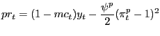
We now describe the profit-maximization problem of intermediate firm j. Due to the constant-returns technology and because we assume zero fixed costs of production, the marginal cost of production, denoted by mct, coincides with average cost. Intermediate firms face a nominal rigidity, modelled using a quadratic cost of price-adjustment. The firm incurs a real cost
| (4) |
in period t of changing its nominal price Pjt-1 to Pjt, which makes its profit-maximization problem a dynamic one. Specifically, in period t, intermediate firm j's problem is to choose Pjt to maximize discounted nominal profits
![$\displaystyle (P_{jt} -P_{t} mc_{t} )y_{jt} -\frac{\psi^{p}}{2}\left( {\frac{P_{jt} }{P_{jt-1} }-1} \right) ^{2}P_{t} +E_{t} \left[ {\frac{q_{t+1} }{\pi _{t+1}^{p} }\left[ {(P_{jt+1} -P_{t+1} mc_{t+1} )y_{jt+1} -\frac{\psi^{p}} {2}\left( {\frac{P_{jt+1} }{P_{jt} }-1} \right) ^{2}P_{t+1} } \right] } \right] $](imgeq5.gif)
| (5) |
where qt+1 denotes the consumer's pricing kernel, derived below, for real risk-free assets and πpt+1 is gross price inflation between period t and t + 1, πpt+1 ≡ Pt+1 / Pt . Because consumers are assumed to own intermediate firms and thus receive their profits, the consumers' nominal discount factor qt+1 / πpt+1 is used to discount period-t + 1 profits. The intermediate firm takes its demand function (2), aggregate demand yt, and the aggregate price level Pt as given.
The first-order-condition of this problem gives rise to a standard New Keynesian Phillips Curve,
![$\displaystyle \left[ {1-\frac{\varepsilon^{p}}{\varepsilon^{p}-1}+\frac{\varepsilon^{p} }{\varepsilon^{p}-1}mc_{t} } \right] y_{t} -\psi^{p}(\pi_{t}^{p} -1)\pi _{t}^{p} +\psi^{p}E_{t} \left[ {q_{t+1} (\pi_{t+1}^{p} -1)\pi_{t+1}^{p} } \right] =0 $](imgeq6.gif)
| (6) |
which we refer to as the price Phillips Curve to distinguish it from an analogous expression for the evolution of nominal wages that arises from the consumer sector of our model.
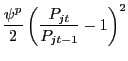
We restrict attention to symmetric equilibria in which all intermediate producers charge the same nominal price and produce the same quantity. Thus, in equilibrium Pjt = Pt and yjt = yt for all j, and there is no price dispersion. In a symmetric equilibrium, real profits of the representative intermediate goods producer in period t + 1, which are distributed to consumers lump-sum in period t + 1, are given by
| (7) |
2.1.3 Employment Agencies
Perfectly-competitive employment agencies hire the differentiated labor of consumers and aggregate them using the CES technology
![$\displaystyle N_{t} =\left[ {\int_{0}^{1} {n_{it}^{1/\varepsilon^{\omega}} di} } \right] ^{\varepsilon^{\omega}} $](imgeq8.gif)
| (8) |
where εω ≥ 1 is the static gross markup of consumer i in the type-i labor market, and εω/(εω - 1) measures the elasticity of substitution between the different types of labor. The final labor input Nt is then sold to intermediate goods producers. Nominal profits of the representative employment agency are given by
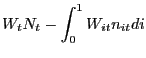
| (9) |
where Wt denotes the aggregate nominal wage rate (the nominal price of Nt) and Wit is the nominal wage of type-i labor. Maximizing (9) with respect to (8) yields the demand function for the i-th consumer's labor,
![$\displaystyle n_{it} =\left[ {\frac{W_{t} }{W_{it} }} \right] ^{\frac{\varepsilon^{\omega} }{\varepsilon^{\omega}-1}}N_{t} $](imgeq10.gif)
| (10) |
As with intermediate producers, we consider only symmetric equilibria in labor markets, in which Wit = Wt and nit = Nt for all i.
2.2 Consumers
There is a continuum of consumers, each of whom supplies to employment agencies his differentiated labor nit according to the demand function (10) after choosing his nominal wage. Each consumer also chooses consumption of cash goods c1t and credit goods c2t, as well as holdings of money Mt and nominal government bonds Bt . We follow the timing described by Chari, Christiano, and Kehoe (1991), in which securities market trading precedes goods and factor market trading. As we make clear below, all consumers make the same decisions, so we do not need to index allocations and asset holdings, except for during optimization with respect to the nominal wage. Thus, each consumer maximizes

| (11) |
subject to the flow budget constraint

| (12) |
the cash-in-advance constraint
| Ptc1t ≤ Mt | (13) |
and the demand function for his labor (10). In (12), the term
 measures the real cost of wage adjustment. Thus, we model sticky wages analogously
to how we model sticky prices, using a quadratic adjustment cost.
Note that in (12), the consumer pays the wage adjustment cost
incurred in period t-1 at the beginning of
period t, in keeping with the timing of Chari,
Christiano, and Kehoe (1991). Wage income is subject to the
proportional tax rate τnt . Real profits of the intermediate goods sector,
prt-1, are received lump-sum with a
one-period lag, and the nominal price of final goods is
measures the real cost of wage adjustment. Thus, we model sticky wages analogously
to how we model sticky prices, using a quadratic adjustment cost.
Note that in (12), the consumer pays the wage adjustment cost
incurred in period t-1 at the beginning of
period t, in keeping with the timing of Chari,
Christiano, and Kehoe (1991). Wage income is subject to the
proportional tax rate τnt . Real profits of the intermediate goods sector,
prt-1, are received lump-sum with a
one-period lag, and the nominal price of final goods is ![]() . Finally, constraint (13) motivates money demand.
. Finally, constraint (13) motivates money demand.
Because we use a quadratic cost of wage adjustment and focus on
a symmetric equilibrium, each consumer is identical to every other
in all his choices, but takes the nominal wages of all others as
given when choosing his optimal nominal wage. Each consumer thus
chooses sequences for c1t, c2t, Wit, Mt and Bt to maximize (11)
subject to (10), (12), and (13). Given optimal choices for these
sequences, the household's labor supply ![]() t is given
by the demand function (10).
t is given
by the demand function (10).
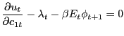
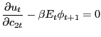
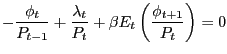
Associate the Lagrange multipliers φt/Pt-1 with the sequence of budget constraints and λt/Pt-1 with the sequence of cash-in-advance constraints. The first-order conditions with respect to cash good consumption, credit good consumption, money holdings, and bond holdings are thus:
| (14) |
| (15) |
| (16) |

| (17) |
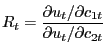
The optimality condition surrounding labor supply is described in Section 2.2.1. From (17), we get the usual Fisher relation,
![$\displaystyle 1=\beta R_{t} E_{t} \left[ {\frac{\phi_{t+1} }{\phi_{t} }\frac{1}{\pi_{t}^{p} }} \right] $](imgeq18.gif)
| (18) |
where πpt ≡ Pt/Pt-1 is the gross
rate of price inflation between period t-1 and period t. The stochastic discount factor ![]() prices a nominal, risk-free one-period asset. We can express the
Fisher relation alternatively in terms of marginal utilities.
Combining (14) and (16), we get
prices a nominal, risk-free one-period asset. We can express the
Fisher relation alternatively in terms of marginal utilities.
Combining (14) and (16), we get

| (19) |
Substituting this expression into (18) gives us the pricing formula for a one-period risk-free nominal bond,
![$\displaystyle 1=\beta R_{t} E_{t} \left[ {\frac{\partial u_{t+1} /\partial c_{1t+1} }{\partial u_{t} /\partial c_{1t} }\frac{1}{\pi_{t+1}^{p} }} \right] $](imgeq20.gif)
| (20) |
the form of the Fisher equation we use in constructing the Ramsey problem in Section 3. As alluded to in the description of intermediate firms above, deFIne the nominal pricing kernel between t and t+1 as
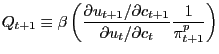
| (21) |
and thus the real pricing kernel as
| (22) |
The consumer first-order conditions also imply that the gross nominal interest rate equals the marginal rate of substitution between cash and credit goods. Specifically,
| (23) |
a standard condition in cash-good/credit-good models. Note that in a monetary equilibrium, Rt ≥ 1, otherwise consumers could earn unbounded profits by buying money and selling bonds.
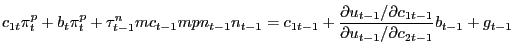
2.2.1 Wage Phillips Curve
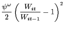
The consumer's first-order-condition with respect to his nominal wage Wit can be expressed as the wage Phillips Curve,
![$\displaystyle \left[ {-\frac{\varepsilon^{\omega}}{mc_{t} mpn_{t} }\frac{\partial u_{t} }{\partial n_{t} }-\left( {1-\tau_{t}^{n} } \right) \frac{\partial u_{t} }{\partial c_{2t} }} \right] n_{t} -\psi^{\omega}\frac{\varepsilon^{\omega} -1}{mc_{t-1} mpn_{t-1} }\frac{\partial u_{t} }{\partial c_{2t} }\left( {\pi_{t}^{\omega}-1} \right) \pi_{t}^{p} +\beta\psi^{\omega}\frac {\varepsilon^{\omega}-1}{mc_{t} mpn_{t} }E_{t} \left[ {\frac{\partial u_{t+1} }{\partial c_{2t+1} }\left( {\pi_{t+1}^{\omega}-1} \right) \pi_{t+1}^{\omega }} \right] =0 $](imgeq24.gif)
| (24) |
in which πωt denotes gross nominal wage inflation between time t-1 and t and πpt denotes gross nominal price inflation between t-1 and t. In deriving the wage Phillips Curve, we use the identity
| (25) |
to substitute out the real wage, and we impose symmetric equilibrium, in which Wit = Wt and nit = Nt for all i. The wage Phillips Curve is forward-looking in that when setting Wit, labor suppliers consider the future nominal wage Wit+1 they expect to charge. This forward-looking aspect of wage-setting is analogous to that embodied in the standard New Keynesian price Phillips Curve (6). With nominal wage inflation determined by the forward-looking wage Phillips Curve, hours worked are determined residually from the demand curve.
2.3 Government
The government's flow budget constraint is
| (26) |
Thus, the government finances government spending through labor income taxation, issuance of nominal debt, and money creation. Note that government consumption is a credit good, following Chari, Christiano, and Kehoe (1991), so that the gt-1 is not paid for until period t. Also, as in Schmitt-Grohe and Uribe (2004b), we assume the government does not have the ability to tax profits of the intermediate goods producers.
Using the first-order conditions of the consumer, we can express the government budget constraint as
| (27) |
which we use in our formulation of the Ramsey problem, described in Section 3. In (27), bt ≡ Bt/Pt denotes the time-t real value of nominal government debt that comes due in period t+1.
2.4 Resource Constraint
Summing the time-t consumer budget constraint and the time-t government budget constraint gives the economy-wide resource constraint,

| (28) |
in which the resource costs associated with price and wage adjustment appear. Note that this resource frontier describes production possibilities for period-t - 1 because of the timing of markets in our model -- specifically, because (all) goods are paid for with a one period lag, summing the time-t consumer and government budget constraints gives rise to the time-t - 1.3
2.5 Competitive Monetary Equilibrium
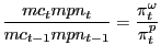
A symmetric competitive monetary equilibrium in our model is a set of endogenous processes {c1t, c2t, nt, Mt, Bt, mct, πpt, πωt} satisfying (6), (14) -(17), (24), (26), and (28), for given policy {τnt, Rt} and exogenous processes {gt, zt}. The restriction Rt ≥ 1 must also be satisfied. Finally, the evolution of real wages is governed by

| (29) |
which states that growth in real wages depends on by how much growth in nominal wages exceeds growth in nominal prices. This expression is of course an identity, but with both a price-setting equation (the price Phillps Curve) and a wage-setting equation (the wage Phillips Curve), the real wage becomes a state variable, requiring a law of motion as part of the description of equilibrium. In the next section, we discuss the economic intuition for why the law of motion for real wages is a necessary component of the definition of equilibrium in the presence of sticky wages.
3 Ramsey Problem
We now describe our formulation of the Ramsey problem. An important constraint on the Ramsey problem that arises with sticky wages is the law of motion for real wages (29), which does not hold trivially in our model. Indeed, Erceg, Henderson, and Levin (2000) also impose such a constraint in their model of optimal monetary policy with sticky wages and sticky prices. Because this restriction is important for the results we obtain and because we find it illuminating for the determination of nominal wages in monetary models generally, we describe more fully the economic intuition behind it.
Consider a model with both flexible prices and flexible wages, but with a nontrivial demand for money. In such an environment, the only economic force acting on either price inflation or wage inflation is the money demand function, which influences price inflation. Supposing the real wage, and hence real wage growth, is pinned down by real features of the economy, nominal wage inflation is free to adjust as a residual to make the law of motion (29) hold. If instead the environment features sticky prices and flexible wages, as in Schmitt-Grohe and Uribe (2004b) and Siu (2004), there are two economic forces acting on price inflation: the money demand function and price-setting behavior on the part of firms. These two forces are balanced against each other, and price inflation is determined. Suppose real wage growth continues to be pinned down by real features of the economy. Wage inflation is thus again free to adjust as a residual to make condition (29) hold.
However, suppose the environment features sticky wages, with either flexible or sticky prices, and real wage growth is still pinned down by real factors. Now there is an independent economic force exerting influence on wage inflation, namely wage-setting behavior on the part of labor suppliers. With wage-setting behavior influencing wage inflation coupled with forces influencing price inflation (money demand either alone or in combination with price-setting behavior), in general wage inflation and price inflation will not be consistent with condition (29). Thus, (29) is a nontrivial condition describing equilibrium and so must be imposed as a constraint on the optimal policy problem.
Our numerical results support our intuition about this constraint. In our flexible-wage models, the Lagrange multiplier associated with this constraint in the Ramsey problem is zero both in steady-state and dynamically, meaning this constraint is redundant. In contrast, with sticky wages, the Lagrange multiplier on this constraint is strictly positive both in steady-state and dynamically, meaning this constraint is required. Intuitively, this condition simply says that as long as real wage growth is not too volatile, the dynamic properties of nominal price inflation and nominal wage inflation will be similar. This idea is the key behind our dynamic results. To express condition (29) in a more convenient form for the Ramsey problem, we use (25) to substitute for the real wage, so we have
| (30) |
We now complete our description of the Ramsey problem. We cannot
eliminate the policy variables πpt, πωt, and τnt from the equilibrium conditions
of the economy because they appear in the forward-looking price
Phillips Curve and wage Phillips Curve. Thus, we cannot adopt the
strict primal approach, in which it is only optimal allocations
that are directly solved for. We instead organize the dynamic
equilibrium conditions into constraints on the Ramsey government
and solve a hybrid of the primal and the dual problem, optimizing
with respect to both allocations and policy variables that cannot
be eliminated. These constraints, in addition to condition (30),
are the resource constraint, the Fisher equation, the wage Phillips
Curve, the price Phillips Curve, and the government budget
constraint. The Ramsey problem is thus to choose sequences ![]() to maximize
to maximize
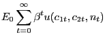
| (31) |
subject to (6), (20), (24), (27), (28), and (30), and given sequences {gt, zt}. In principle, we must also impose the constraint Rt ≥ 1, which ensures the chosen allocation can be supported as a monetary equilibrium. However, because in our models Rt > 0 in steady-state and the volatilities of the exogenous processes are suffciently small, the lower bound Rt = 1 was never reached in any of our simulations of the model omitting this constraint.
A technical issue that arises in the formulation of this hybrid Ramsey problem is the dating of the Lagrange multiplier associated with the resource constraint. Recall from Section 2.4 that it is the time-t - 1 resource frontier that is implied by the time-t consumer and government flow budget constraints. Because the assumed timing of our model is that the Ramsey planner observes gt before choosing time-t allocations and policies, the multiplier associated with constraint (28) is dated t - 1 - in other words, terms in the Ramsey first-order-conditions arising from the resource constraint carry a multiplier dated t.
4 Quantitative Results
We briefly describe the functional forms and parameter values we use, which are standard in the literature, to obtain our main results. We then analyze optimal policy in the Ramsey steady-state before presenting our simulation-based dynamic results.
4.1 Parameterization
We use a period utility function
| (32) |
with the consumption index is a CES aggregate of cash goods and credit goods,
| (33) |
We set σ = 1 so that preferences are separable in leisure and consumption. In the consumption aggregator, we use φ = 0.79 and γ = 0.62, as estimated by Siu (2004). The parameter ξ is calibrated so that in the non-stochastic Ramsey steady-state the consumer spends 30 percent of his time working. The time unit is one quarter, so we set the subjective time discount factor to β = 0.99.
The aggregate productivity and government spending shocks follow AR(1) processes in logs,
| (34) |
| (35) |
where ![]() denotes the steady-state level of government
spending, which is calibrated to be 20 percent of steady-state
output. The innovations
denotes the steady-state level of government
spending, which is calibrated to be 20 percent of steady-state
output. The innovations ![]() and
and ![]() are distributed
are distributed ![]() and
and ![]() , respectively. We choose parameters ρz = 0.95, ρg = 0.97,
, respectively. We choose parameters ρz = 0.95, ρg = 0.97, ![]() = 0.007, and
= 0.007, and ![]() = 0.02 in keeping with the RBC literature and Chari, Christiano,
and Kehoe (1991).
= 0.02 in keeping with the RBC literature and Chari, Christiano,
and Kehoe (1991).
Finally, it remains to choose parameter values governing the degree of imperfect competition and nominal rigidity in product markets and labor markets. For our main results, we set the gross markup in labor markets to εω = 1.05 and the gross markup in intermediate goods markets to εp = 1.1, in keeping with the findings of Christiano, Eichenbaum, and Evans (2005). Also in line with their findings, we calibrate ψω and ωp so that on average nominal wages and nominal prices are fixed for three quarters.4 As we report below, we conduct experiments in which one or the other, prices or wages, is flexible, in which case we leave the average length of stickiness of the other at three months.
4.2 Optimal Steady-State Policy
Using the nonlinear Ramsey first-order conditions, we numerically compute the non-stochastic Ramsey steady-state allocation and policy. Table 1 presents the steady-state labor tax rate, price inflation rate, wage inflation rate, and nominal interest rate for various degrees of imperfect competition in our model with both flexible wages and flexible prices.
For a given markup in the labor market, our results resemble
Schmitt-Grohe and Uribe's (2004a) results for imperfectly
competitive product markets. Indeed, as we prove in the Appendix,
goods market power leads to a deviation from the Friedman Rule in
our model. For a given wage markup, the steady-state tax rate,
nominal interest rate, price inflation rate, and wage inflation rate
are all increasing in the degree of product market power. The
reason that the nominal interest rate is increasing in
![]()
![]() is that
in the absence of a 100 percent profit tax, the nominal interest
rate indirectly taxes profit income, as explained in Schmitt-Grohe
and Uribe (2004a). profit income represents payments to a fixed
factor, monopoly power, which the Ramsey planner would like to tax
as heavily as possible because it would be non-distortionary. With
confiscation of profits ruled out, the nominal interest rate acquires
the auxiliary role of indirectly taxing profits. Thus, the Friedman
Rule of a zero net nominal interest rate ceases to be optimal once
product markets exhibit monopoly power. With the steady-state real
interest rate pinned down by the subjective discount factor and
independent of monopoly power, steady-state price inflation thus
also rises above the Friedman deflation as
is that
in the absence of a 100 percent profit tax, the nominal interest
rate indirectly taxes profit income, as explained in Schmitt-Grohe
and Uribe (2004a). profit income represents payments to a fixed
factor, monopoly power, which the Ramsey planner would like to tax
as heavily as possible because it would be non-distortionary. With
confiscation of profits ruled out, the nominal interest rate acquires
the auxiliary role of indirectly taxing profits. Thus, the Friedman
Rule of a zero net nominal interest rate ceases to be optimal once
product markets exhibit monopoly power. With the steady-state real
interest rate pinned down by the subjective discount factor and
independent of monopoly power, steady-state price inflation thus
also rises above the Friedman deflation as
![]()
![]() increases. Because real wages are by construction
constant in the steady-state, nominal wages must grow at the same
rate as nominal prices. Finally, the labor income tax rate is also
increasing in the degree of market power, again consistent with
Schmitt-Grohe and Uribe (2004a). However, the reason for this is a
little more subtle in our model than in their model. In their
study, the fraction of time spent working decreases as market power
increases, so their claim is that both the decline in hours and the
decline in wages (due to stronger market power) call for a higher
tax rate to raise a given revenue. However, because we re-calibrate
increases. Because real wages are by construction
constant in the steady-state, nominal wages must grow at the same
rate as nominal prices. Finally, the labor income tax rate is also
increasing in the degree of market power, again consistent with
Schmitt-Grohe and Uribe (2004a). However, the reason for this is a
little more subtle in our model than in their model. In their
study, the fraction of time spent working decreases as market power
increases, so their claim is that both the decline in hours and the
decline in wages (due to stronger market power) call for a higher
tax rate to raise a given revenue. However, because we re-calibrate
![]() so that steady-state hours are
constant across all parameterizations, we can conclude that the
higher tax rate is required only because of the decline in
wages.5 In either case, it is a shrinking labor
tax base that calls for a higher labor tax rate.
so that steady-state hours are
constant across all parameterizations, we can conclude that the
higher tax rate is required only because of the decline in
wages.5 In either case, it is a shrinking labor
tax base that calls for a higher labor tax rate.
Table 1: Steady-state optimal policy for various values of εp and εω
Nominal interest rate, price inflation rate, and wage inflation rate reported in annualized percentage points.
| Gross Labor Markup, Variable | Gross Product Markup: εp = 1 | Gross Product Markup: εp = 1.1 | Gross Product Markup: εp = 1.2 |
|---|---|---|---|
| εω = 1, τn | 0.2228 | 0.2446 | 0.2661 |
| εω = 1, R | 0 | 0.8305 | 2.0721 |
| εω = 1, πp | -4 | -3.2033 | -2.011 |
| εω = 1, πω | -4 | -3.2033 | -2.011 |
| εω = 1.05, τn | 0.2228 | 0.2445 | 0.2660 |
| εω = 1.05, R | 0 | 0.9140 | 2.2138 |
| εω = 1.05, πp | -4 | -3.1223 | -1.8748 |
| εω = 1.05, πω | -4 | -3.1223 | -1.8748 |
| εω = 1.1, τn | 0.2228 | 0.2445 | 0.2660 |
| εω = 1.1, R | 0 | 0.9894 | 2.3412 |
| εω = 1.1, πp | -4 | -3.0502 | -1.7525 |
| εω = 1.1, πω | -4 | -3.0502 | -1.7525 |
| εω = 1.2, τn | 0.2228 | 0.2444 | 0.2658 |
| εω = 1.2, R | 0 | 1.1203 | 2.5609 |
| εω = 1.2, πp | -4 | -2.9245 | -1.5415 |
| εω = 1.2, πω | -4 | -2.9245 | -1.5415 |
4.2.1 Taxation of Labor Market Power
We can also analyze how the steady-state policy responds to
labor market power. Along this dimension, there is an asymmetry in
the policy response depending on whether or not product markets
exhibit monopoly power. As the first column of Table 1 shows, the
labor tax rate is invariant to
![]()
![]() if goods
markets are perfectly competitive. However, this result is a direct
consequence of our re-calibrating
if goods
markets are perfectly competitive. However, this result is a direct
consequence of our re-calibrating ![]() in every
version of our model to hold steady-state hours constant at n = 0.30. Indeed, the value
in every
version of our model to hold steady-state hours constant at n = 0.30. Indeed, the value ![]() , which governs the disutility of work, declines as
the degree of labor market power increases to ensure that
steady-state hours are constant. In Table 2, we instead hold
, which governs the disutility of work, declines as
the degree of labor market power increases to ensure that
steady-state hours are constant. In Table 2, we instead hold
![]() fixed at its calibrated value in the
perfectly-competitive economy and compute the steady-state Ramsey
policy for various values of
fixed at its calibrated value in the
perfectly-competitive economy and compute the steady-state Ramsey
policy for various values of
![]()
![]() . Labor
hours decline as
. Labor
hours decline as
![]()
![]() rises, as
expected, but nonetheless the labor tax rate rises. A rise in the
labor tax rate would seem counterintuitive because with labor
supply smaller than the Pareto optimum, one might expect the Ramsey
planner to reduce the labor tax rate to subsidize labor. However,
with labor market power representing a fixed factor of production,
the Ramsey planner has an incentive to tax labor more heavily
because part of the tax falls on monopoly rents and thus is
non-distortionary. Our numerical results show that the latter effect
dominates and the labor tax rate rises in Table 2. This result is
related to the Schmitt-Grohe and Uribe (2004a) result that the
Ramsey planner taxes market power -- in their case, product market
power, in our case, labor market power -- through available
instruments.
rises, as
expected, but nonetheless the labor tax rate rises. A rise in the
labor tax rate would seem counterintuitive because with labor
supply smaller than the Pareto optimum, one might expect the Ramsey
planner to reduce the labor tax rate to subsidize labor. However,
with labor market power representing a fixed factor of production,
the Ramsey planner has an incentive to tax labor more heavily
because part of the tax falls on monopoly rents and thus is
non-distortionary. Our numerical results show that the latter effect
dominates and the labor tax rate rises in Table 2. This result is
related to the Schmitt-Grohe and Uribe (2004a) result that the
Ramsey planner taxes market power -- in their case, product market
power, in our case, labor market power -- through available
instruments.
Further evidence for the use of the labor tax to extract part of
the monopoly surplus of labor power comes from modifying our model
slightly to allow for a proportional labor subsidy to undo the
static distortion due to the markup. In particular, suppose the
government subsidizes labor income at the rate 1 + ![]()
![]() , so that total nominal labor income
of the consumer is given by
, so that total nominal labor income
of the consumer is given by
| (36) |
Setting a labor subsidy 1 + ![]()
![]() =
=
![]()
![]() to
completely offet labor market power yields a labor tax rate
to
completely offet labor market power yields a labor tax rate
![]()
![]() invariant to
invariant to
![]() .6 Thus, absent the offsetting subsidy, the labor tax rate
adjusts to tax away part of the labor rent. Apparently, a higher
labor tax rate balances the benefit of taxing this pure rent against
the cost of a larger distortion in the consumption-leisure
margin.
.6 Thus, absent the offsetting subsidy, the labor tax rate
adjusts to tax away part of the labor rent. Apparently, a higher
labor tax rate balances the benefit of taxing this pure rent against
the cost of a larger distortion in the consumption-leisure
margin.
On the other hand, examining either Table 1 or 2, we find that
the nominal interest rate, and hence both price inflation and wage
inflation, are invariant to
![]()
![]() when
product markets are perfectly competitive because there are no
producer profits to (indirectly) tax. This result is overturned,
however, when product markets are imperfectly competitive, as we
now discuss.
when
product markets are perfectly competitive because there are no
producer profits to (indirectly) tax. This result is overturned,
however, when product markets are imperfectly competitive, as we
now discuss.
With monopoly power in product markets (the second and third
columns of Table 1), the nominal interest rate and both price and
wage inflation all rise slightly as
![]()
![]() rises.
The rise in the nominal interest rate is not due to an increase in
the (indirect) tax on monopoly producers' profits because for a
given
rises.
The rise in the nominal interest rate is not due to an increase in
the (indirect) tax on monopoly producers' profits because for a
given
![]()
![]() in Table
1, profits are constant due to our re-calibration of
in Table
1, profits are constant due to our re-calibration of ![]() . Rather, the rise in R is due to the Ramsey planner
taxing labor market power indirectly through the nominal interest
rate. We can show this by again introducing the labor subsidy
. Rather, the rise in R is due to the Ramsey planner
taxing labor market power indirectly through the nominal interest
rate. We can show this by again introducing the labor subsidy
![]()
![]() as described
above, which effectively removes the labor power. Setting the
subsidy 1 +
as described
above, which effectively removes the labor power. Setting the
subsidy 1 + ![]()
![]() =
=
![]()
![]() , we find
that R is invariant to
, we find
that R is invariant to
![]() for a given
for a given
![]() , confirming our intuition. As
mentioned above, Schmitt-Grohe and Uribe (2004a) find that
deviations from the Friedman Rule indirectly tax monopoly
producers' profits. We uncover a related result regarding the use of
nominal interest rates to indirectly tax monopoly labor suppliers'
rents. Interestingly, however, positive producer profits are
necessary for the ability of R to tax labor power because with
perfect competition in product markets R does not vary with εω, as Table 1 shows.7 Thus, labor market power alone does not
induce deviations from the Friedman Rule, but once the Friedman
Rule has already been abandoned, increasing labor power induces
further deviations from the Friedman Rule.
, confirming our intuition. As
mentioned above, Schmitt-Grohe and Uribe (2004a) find that
deviations from the Friedman Rule indirectly tax monopoly
producers' profits. We uncover a related result regarding the use of
nominal interest rates to indirectly tax monopoly labor suppliers'
rents. Interestingly, however, positive producer profits are
necessary for the ability of R to tax labor power because with
perfect competition in product markets R does not vary with εω, as Table 1 shows.7 Thus, labor market power alone does not
induce deviations from the Friedman Rule, but once the Friedman
Rule has already been abandoned, increasing labor power induces
further deviations from the Friedman Rule.
Table 2: Steady-state optimal policy holding ξ = 2.2667 and εp = 1 fixed.
Nominal interest rate, price inflation rate, and wage inflation rate reported in annualized percentage points.
| Policy | τn | R | πp | πω | n |
|---|---|---|---|---|---|
| εω = 1 | 0.2228 | 0 | -4 | -4 | 0.3000 |
| εω = 1.05 | 0.2235 | 0 | -4 | -4 | 0.2897 |
| εω = 1.1 | 0.2243 | 0 | -4 | -4 | 0.2800 |
| εω = 1.2 | 0.2253 | 0 | -4 | -4 | 0.2675 |
Table 3: Steady-state optimal policy in sticky-price and/or sticky-wage economies, for εp = 1.1 and εω = 1.05
Nominal adjustment parameters set so that the respective nominal rigidity lasts for three quarters on average. Nominal interest rate, price inflation rate, and wage inflation rate reported in annualized percentage points.
| Policy | τn | R | πp | πω |
|---|---|---|---|---|
| Sticky price, flexible wage | 0.2496 | 4.1297 | -0.0355 | -0.0355 |
| Flexible price, sticky wage | 0.2429 | 4.1369 | -0.0285 | -0.0285 |
| Sticky price, sticky wage | 0.2256 | 4.1007 | -0.0013 | -0.0013 |
Finally, Table 3 displays the Ramsey policy when either or both
prices and wages are sticky, with the static markups at our
baseline values of
![]()
![]() =1
=1![]() 05 and
05 and
![]()
![]() =1
=1![]() 1. With either sticky prices or sticky
wages, or both, near-perfect nominal price stability and nominal
wage stability are optimal. That the steady-state price and wage
inflation rates are identical follows immediately from a constant
real wage in condition (29), which explains how a motive to
stabilize only nominal wages translates into stabilization of
nominal prices. This channel is also crucial for understanding our
dynamic results, to which we turn next.
1. With either sticky prices or sticky
wages, or both, near-perfect nominal price stability and nominal
wage stability are optimal. That the steady-state price and wage
inflation rates are identical follows immediately from a constant
real wage in condition (29), which explains how a motive to
stabilize only nominal wages translates into stabilization of
nominal prices. This channel is also crucial for understanding our
dynamic results, to which we turn next.
4.3 Inflation Volatility
We simulate our models by linearizing in levels the Ramsey first-order conditions for time t > 0 around the non-stochastic steady-state of these conditions. We adopt the timeless perspective described by Woodford (2003) by assuming that the initial state of the economy is the asymptotic Ramsey steady-state; we also point out that because we assume full commitment, the use of state-contingent inflation is not a manifestation of time-inconsistent policy. Linear decision rule are obtained using the perturbation algorithm described by Schmitt-Grohe and Uribe (2004c).
4.3.1 Both Government Spending and Productivity Shocks
Table 4 presents simulation-based moments for the key policy variables along with the real wage for several versions of our model when the driving forces of the economy are both technology shocks and government spending shocks.8 We start with this case because it is the case often focused on in the existing Ramsey literature. In the next subsection, we focus on the case where the economy is driven by only government spending shocks, which is the core motive for the use of state-contingent inflation.
The top panel of Table 4 presents results for the model with perfect competition in both product and labor markets. As originally found by Chari, Christiano, and Kehoe (1991), price inflation is quite volatile and the labor tax rate very stable in this economy. The reason for this, as described in the introduction and well-known in the Ramsey literature, is that the Ramsey planner uses surprise variations in the price level to render nominally risk-free debt state-contingent in real terms, thus financing a large portion of innovations to government spending in a non-distortionary way and permitting tax-smoothing. The new result we display in the top panel is that nominal wage inflation, because it is highly correlated with price inflation through condition (30), is also quite volatile. These results, high volatility of both price inflation and wage inflation, carry over to the economy with monopoly power but flexible prices in both goods and labor markets, the second panel in Table 4.
The third panel in Table 4 displays results for the model with
sticky prices and flexible wages. Consistent with the findings of
Schmitt-Grohe and Uribe (2004b) and Siu (2004), the volatility of
price inflation falls by an order of magnitude, and the mean
inflation rate rises from close to the Friedman deflation to near
zero. The reason for this is that with costs of nominal price
adjustment, the Ramsey planner keeps price changes to a minimum in
levying the inflation tax on nominal wealth. Nominal wage inflation
volatility also falls, although not as dramatically -- its
volatility of 1.07 percent is about two-thirds the volatility with flexible
prices. The tradeoff facing the Ramsey planner here seems to be the
one described by Erceg, Henderson, and Levin (2000): in engineering
the optimal real wage, fluctuations in nominal prices are
undesirable because of the cost of price adjustment, thus the
Ramsey planner resorts to fluctuations in nominal wages, which are
costless. With smaller variations in inflation, however, more of the
surprise revenue generation falls on the labor tax rate, thus the
rise in the volatility of ![]()
![]() . Note, however, that the fluctuations in inflation here
are not driven solely by government revenue requirements because
productivity is also fluctuating. In the next subsection, we focus on the case of
only government spending shocks.
. Note, however, that the fluctuations in inflation here
are not driven solely by government revenue requirements because
productivity is also fluctuating. In the next subsection, we focus on the case of
only government spending shocks.
The fourth panel of Table 4 shows results for the model with flexible prices and sticky wages. A natural conjecture for this case is that price inflation volatility is intermediate between the fully-flexible case and the sticky-price/flexible-wage case. Our numerical results show this to be true, with price inflation volatility about one-third that in the fully-flexible economy. This result contrasts with that found by Schmitt-Grohe and Uribe (2005). They find that with sticky wages and flexible prices, price inflation volatility is virtually the same as that under full flexibility -- namely, highly volatile price inflation -- when the economy is driven by both government spending and productivity shocks. Because our model does not consider the other frictions their model considers, our results suggest that stickiness in nominal wages alone does dampen Ramsey inflation volatility, but this effect can be overridden by other frictions present in the environment. We find that wage inflation volatility for this case is quite small, as would be expected due to the assumed wage rigidity, and is an order of magnitude smaller than price inflation volatility. This is the reverse of the results with sticky prices and flexible wages and seems to be driven by the same concern of the Ramsey planner for implementing a real wage as close as possible to the efficient real wage: with stickiness in only wages, the Ramsey planner generates some volatility in prices, but not as much as predicted by the Schmitt-Grohe and Uribe (2005) model. We further disentangle the effects of the exogenous shocks on price inflation and wage inflation volatility in this flexible-price/sticky-wage case in the next subsection. Note also that the volatility of the labor tax rate in this case is about the same as in the sticky-price/flexible-wage case.
Finally, the bottom panel of Table 4 presents results for the model with both sticky prices and sticky wages. Here, we find that wage inflation is quite volatile, even more volatile than in the fully-flexible environment. However, this result is due to the interaction of technology shocks with sticky prices and sticky wages. Notice that the volatility of the real wage w is largest in this case. Evidently, the interaction of technology shocks with stickiness in both product and labor markets leads the Ramsey planner to stabilize nominal price inflation to a large degree. However, with a relatively volatile real wage, the policy therefore calls for volatile nominal wages.
4.3.2 Disentangling the effects of Shocks
Table 4 is comparable to Table 4A in Schmitt-Grohe and Uribe (2005) in that it considers the responses of the Ramsey allocation to both technology and government spending shocks. The core motive of the use of surprise changes in the price level in a Ramsey model, however, is to finance government spending shocks in a non-distortionary way. Indeed, Siu (2004) considers only government spending shocks in his study. Thus, we find it instructive to examine the effect of sticky wages when the economy is buffeted by only government spending shocks or only technology shocks. To this end, Tables 5 and 6 present simulation-based moments when there is only one driving process in the model, only government spending shocks in Table 5 and only technology shocks in Table 6.
Table 4: Simulation-based moments with gt and zt as the driving processes - Panel A: Perfect Competition
πp, πω, and R reported in annualized percentage points. Markup parameters are εω = 1.05 and εp = 1.1. For either sticky wages or sticky prices, ψω and/or ψp are set so that the respective nominal rigidity lasts nine months on average.
| Variable | Mean | Std. Dev. | Auto corr. | Corr(x, y) | Corr(x, g) | Corr(x, z) |
|---|---|---|---|---|---|---|
| τn | 0.2229 | 0.0024 | 0.8242 | -0.1435 | 0.8431 | -0.5304 |
| πp | -3.9705 | 2.2042 | 0.0329 | 0.0507 | 0.0465 | 0.0380 |
| πω | -3.9681 | 1.5719 | 0.1465 | 0.2729 | 0.0687 | 0.2711 |
| R | 0 | 0 | - | - | - | - |
| ω | 1.0010 | 0.0161 | 0.7718 | 0.9066 | -0.0170 | 1 |
Table 4: Simulation-based moments with gt and zt as the driving processes - Panel B: Flexible prices, Flexible wages
| Variable | Mean | Std. Dev. | Auto corr. | Corr(x, y) | Corr(x, g) | Corr(x, z) |
|---|---|---|---|---|---|---|
| τn | 0.2446 | 0.0037 | 0.8217 | -0.3020 | 0.8180 | -0.5672 |
| πp | -3.0919 | 2.3404 | 0.0748 | 0.0748 | -0.0102 | 0.0840 |
| πω | -3.0894 | 1.7244 | 0.2085 | 0.2948 | -0.0099 | 0.3140 |
| R | 0.9170 | 0.0299 | 0.8091 | 0.4851 | -0.6841 | 0.7212 |
| ω | 0.9100 | 0.0146 | 0.7718 | 0.9522 | -0.0170 | 1 |
Table 4: Simulation-based moments with gt and zt as the driving processes - Panel C: Sticky prices, Flexible wages
| Variable | Mean | Std. Dev. | Auto corr. | Corr(x, y) | Corr(x, g) | Corr(x, z) |
|---|---|---|---|---|---|---|
| τn | 0.2449 | 0.0048 | 0.5476 | -0.4217 | 0.7322 | -0.5788 |
| πp | -0.0274 | 0.1973 | 0.7888 | 0.8245 | -0.2813 | 0.8787 |
| πω | -0.0151 | 1.0715 | 0.1843 | 0.5824 | -0.0416 | 0.6442 |
| R | 3.9501 | 0.3878 | 0.8838 | -0.7917 | 0.2621 | -0.8378 |
| ω | 0.9099 | 0.0170 | 0.8291 | 0.9599 | -0.0067 | 0.9693 |
Table 4: Simulation-based moments with gt and zt as the driving processes - Panel D: Flexible prices, Sticky wages
| Variable | Mean | Std. Dev. | Auto corr. | Corr(x, y) | Corr(x, g) | Corr(x, z) |
|---|---|---|---|---|---|---|
| τn | 0.2429 | 0.0046 | 0.4888 | -0.5696 | 0.5247 | -0.1966 |
| πp | -0.0272 | 0.7922 | -0.0677 | 0.3353 | -0.0226 | -0.2743 |
| πω | -0.0254 | 0.0805 | 0.5164 | 0.8300 | -0.1835 | 0.4100 |
| R | 3.7627 | 0.8374 | 0.6460 | -0.8766 | 0.2056 | -0.5210 |
| ω | 0.9098 | 0.0102 | 0.7718 | 0.7857 | -0.0170 | 1 |
Table 4: Simulation-based moments with gt and zt as the driving processes - Panel E: Sticky prices, Sticky wages
| Variable | Mean | Std. Dev. | Auto corr. | Corr(x, y) | Corr(x, g) | Corr(x, z) |
|---|---|---|---|---|---|---|
| τn | 0.2260 | 0.0025 | 0.9268 | 0.8354 | 0.6032 | 0.6911 |
| πp | -0.0483 | 0.5020 | 0.5890 | -0.6519 | -0.0640 | -0.8363 |
| πω | 0.3770 | 2.6724 | 0.8907 | 0.9253 | -0.0449 | 0.9988 |
| R | 4.5456 | 0.2576 | 0.9308 | -0.9262 | 0.1296 | -0.8800 |
| ω | 0.9121 | 0.0217 | 0.9663 | 0.9744 | -0.0316 | 0.9485 |
First consider the fully-flexible cases, the top two panels of Tables 5 and 6. When the economy is hit with only government spending shocks, the dynamics of price inflation are identical to the dynamics of wage inflation. This is to be expected because by assumption the marginal product of labor is constant and the marginal cost of production is constant because prices are flexible.9 The real wage is thus constant, and condition (29) then reveals that price inflation and wage inflation track each other perfectly. The dynamics of wage and price inflation differ, of course, when the real wage is fluctuating, as is the case in Table 6 with technology shocks -- note that both price inflation and wage inflation are quite volatile, as is expected with flexible prices and wages.
Turning to the third panel of Table 5, we find that sticky prices dampen price inflation volatility by an order of magnitude, also as expected. Because the marginal cost of production mct fluctuates over time due to sticky prices, the dynamics of wage inflation are not identical to those of price inflation. Nonetheless, the volatility of wage inflation also falls substantially, although not by as much as the volatility of price inflation. Comparing the results here with those in the third panel of Table 6, we see that neither price inflation nor wage inflation is dampened as much with technology shocks as the sole driving force, but they are both lower than the fully-flexible cases.
Examining the fourth panel of Table 5 reveals the source of our
main result. With stickiness in only nominal wages, the dynamics of
price inflation and wage inflation are identical because the marginal
cost of production is constant and equal to the inverse of the
gross product markup
![]()
![]() . The
marginal product of labor is constant by assumption because we have
shut down productivity shocks. A natural conjecture may be that
even with technology shocks shut down, the real wage would fluctuate
because of innovations to government spending. However, government
spending shocks are fundamentally non-distortionary shocks. They
become potentially distortionary only if lump-sum taxes are ruled
out, as they are in the canonical Ramsey environment.10 But in our environment the Ramsey planner has back-door
ways of generating lump-sum revenues -- the inflation tax on
bond-holders and the departure from the Friedman Rule that
indirectly taxes monopoly power in both product and labor markets.
Thus, with only government spending shocks and access to ways to
generate lump-sum revenues, the Ramsey planner would like to keep
the real wage from fluctuating, which requires that the dynamics of
price inflation and wage inflation be identical. With a cost of
adjusting nominal wages, however, the Ramsey planner is reluctant
to generate wage inflation, and thus also reluctant to generate price
inflation because of the restriction (29).
. The
marginal product of labor is constant by assumption because we have
shut down productivity shocks. A natural conjecture may be that
even with technology shocks shut down, the real wage would fluctuate
because of innovations to government spending. However, government
spending shocks are fundamentally non-distortionary shocks. They
become potentially distortionary only if lump-sum taxes are ruled
out, as they are in the canonical Ramsey environment.10 But in our environment the Ramsey planner has back-door
ways of generating lump-sum revenues -- the inflation tax on
bond-holders and the departure from the Friedman Rule that
indirectly taxes monopoly power in both product and labor markets.
Thus, with only government spending shocks and access to ways to
generate lump-sum revenues, the Ramsey planner would like to keep
the real wage from fluctuating, which requires that the dynamics of
price inflation and wage inflation be identical. With a cost of
adjusting nominal wages, however, the Ramsey planner is reluctant
to generate wage inflation, and thus also reluctant to generate price
inflation because of the restriction (29).
Table 5: Simulation-based moments with gt as the only driving process - Panel A: Perfect Competition
πp, πω, and R reported in annualized percentage points. Markup parameters are εω = 1.05 and εp = 1.1. For either sticky wages or sticky prices, ψω and/or ψp are set so that the respective nominal rigidity lasts nine months on average.
| Variable | Mean | Std. Dev. | Auto corr. | Corr(x, y) | Corr(x, g) | Corr(x, z) |
|---|---|---|---|---|---|---|
| τn | 0.2229 | 0.0020 | 0.8415 | 1 | 1 | - |
| πp | -4.0114 | 1.2286 | -0.0298 | 0.0981 | 0.0981 | - |
| πω | -4.0114 | 1.2286 | -0.0298 | 0.0981 | 0.0981 | - |
| R | 0 | 0 | - | - | - | - |
| ω | 1 | 0 | - | - | - | - |
Table 5: Simulation-based moments with gt as the only driving process - Panel B: Flexible prices, Flexible wages
| Variable | Mean | Std. Dev. | Auto corr. | Corr(x, y) | Corr(x, g) | Corr(x, z) |
|---|---|---|---|---|---|---|
| τn | 0.2447 | 0.0031 | 0.8415 | 1 | 1 | - |
| πp | -3.1414 | 1.3178 | 0.0165 | -0.0032 | -0.0032 | - |
| πω | -3.1414 | 1.3178 | 0.0165 | -0.0032 | -0.0032 | - |
| R | 0.9040 | 0.2056 | 0.8415 | -1 | -1 | - |
| ω | 0.9091 | 0 | - | - | - | - |
Table 5: Simulation-based moments with gt as the only driving process - Panel C: Sticky prices, Flexible wages
| Variable | Mean | Std. Dev. | Auto corr. | Corr(x, y) | Corr(x, g) | Corr(x, z) |
|---|---|---|---|---|---|---|
| τn | 0.2497 | 0.0038 | 0.5419 | 0.8907 | 0.9312 | - |
| πp | -0.0382 | 0.0674 | 0.5522 | -0.8035 | -0.7948 | - |
| πω | -0.0386 | 0.3808 | -0.4553 | -0.1335 | -0.1129 | - |
| R | 4.1849 | 0.1198 | 0.7636 | 0.8598 | 0.8137 | - |
| ω | 0.9002 | 0.0024 | -0.3537 | 0.0111 | 0.0766 | - |
Table 5: Simulation-based moments with gt as the only driving process - Panel D: Flexible prices, Sticky wages
| Variable | Mean | Std. Dev. | Auto corr. | Corr(x, y) | Corr(x, g) | Corr(x, z) |
|---|---|---|---|---|---|---|
| τn | 0.2430 | 0.0025 | 0.6853 | 0.6911 | 0.9696 | - |
| πp | -0.0291 | 0.0162 | 0.4466 | -0.4431 | -0.8500 | - |
| πω | -0.0291 | 0.0162 | 0.4466 | -0.4431 | -0.8500 | - |
| R | 4.1971 | 0.1914 | 0.4355 | 0.4292 | 0.8417 | - |
| ω | 0.9091 | 0 | - | - | - | - |
Table 5: Simulation-based moments with gt as the only driving process - Panel E: Sticky prices, Sticky wages
| Variable | Mean | Std. Dev. | Auto corr. | Corr(x, y) | Corr(x, g) | Corr(x, z) |
|---|---|---|---|---|---|---|
| τn | 0.2257 | 0.0016 | 0.8782 | 0.9795 | 0.9964 | - |
| πp | -0.0050 | 0.0406 | 0.9013 | -0.9872 | -0.9990 | - |
| πω | -0.0065 | 0.0617 | 0.7699 | -0.9211 | -0.9605 | - |
| R | 4.4036 | 0.9921 | 0.7300 | 0.8994 | 0.9445 | - |
| ω | 0.9091 | 0.0001 | 0.8210 | -0.9062 | -0.9440 | - |
Table 6: Simulation-based moments with zt as the only driving process - Panel A: Perfect Competition
πp, πω, and R reported in annualized percentage points. Markup parameters are εω = 1.05 and εp = 1.1. For either sticky wages or sticky prices, ψω and/or ψp are set so that the respective nominal rigidity lasts nine months on average.
| Variable | Mean | Std. Dev. | Auto corr. | Corr(x, y) | Corr(x, g) | Corr(x, z) |
|---|---|---|---|---|---|---|
| τn | 0.2228 | 0.0012 | 0.7718 | -1 | - | 1 |
| πp | -3.9592 | 1.8312 | 0.0546 | 0.0450 | - | 0.0450 |
| πω | -3.9567 | 0.9804 | 0.4024 | 0.4298 | - | 0.4298 |
| R | 0 | 0 | - | - | - | - |
| ω | 1 | 0.0161 | 0.7718 | 1 | - | 1 |
Table 6: Simulation-based moments with zt as the only driving process - Panel B: Flexible prices, Flexible wages
| Variable | Mean | Std. Dev. | Auto corr. | Corr(x, y) | Corr(x, g) | Corr(x, z) |
|---|---|---|---|---|---|---|
| τn | 0.2444 | 0.0021 | 0.7718 | -1 | - | -1 |
| πp | -3.0732 | 1.9336 | 0.0940 | 0.0996 | - | 0.0996 |
| πω | -3.0707 | 1.1093 | 0.4583 | 0.4815 | - | 0.4815 |
| R | 0.9270 | 0.2135 | 0.7718 | 1 | - | 1 |
| ω | 0.9100 | 0.0146 | 0.7718 | 1 | - | 1 |
Table 6: Simulation-based moments with zt as the only driving process - Panel C: Sticky prices, Flexible wages
| Variable | Mean | Std. Dev. | Auto corr. | Corr(x, y) | Corr(x, g) | Corr(x, z) |
|---|---|---|---|---|---|---|
| τn | 0.2494 | 0.0025 | 0.5458 | -0.9242 | - | -0.9417 |
| πp | -0.0264 | 0.1568 | 0.8170 | 0.9585 | - | 0.9371 |
| πω | -0.0156 | 0.8536 | 0.2731 | 0.6426 | - | 0.6884 |
| R | 3.9301 | 0.3113 | 0.8941 | -0.9116 | - | -0.8831 |
| ω | 0.8995 | 0.0143 | 0.8530 | 0.9905 | - | -0.7253 |
Table 6: Simulation-based moments with zt as the only driving process - Panel D: Flexible prices, Sticky wages
| Variable | Mean | Std. Dev. | Auto corr. | Corr(x, y) | Corr(x, g) | Corr(x, z) |
|---|---|---|---|---|---|---|
| τn | 0.2428 | 0.0039 | 0.4036 | -0.7635 | - | -0.2274 |
| πp | -0.0267 | 0.7919 | -0.0679 | 0.3407 | - | -0.2747 |
| πω | -0.0248 | 0.0786 | 0.5178 | 0.8769 | - | 0.4165 |
| R | 3.7026 | 0.8123 | 0.6567 | -0.9338 | - | -0.5335 |
| ω | 0.9097 | 0.0102 | 0.7718 | 0.7992 | - | 1 |
Table 6: Simulation-based moments with zt as the only driving process - Panel E: Sticky prices, Sticky wages
| Variable | Mean | Std. Dev. | Auto corr. | Corr(x, y) | Corr(x, g) | Corr(x, z) |
|---|---|---|---|---|---|---|
| τn | 0.2258 | 0.0020 | 0.9630 | 0.9838 | - | 0.9455 |
| πp | -0.0445 | 0.5010 | 0.5887 | -0.6531 | - | -0.8411 |
| πω | 0.3822 | 2.6699 | 0.8906 | 0.9511 | - | 0.9991 |
| R | 4.2204 | 1.1124 | 0.9333 | -0.9789 | - | -0.8864 |
| ω | 0.9121 | 0.0217 | 0.9663 | 0.9981 | - | 0.9485 |
Finally, the fifth panels of Tables 5 and 6 show that with both sticky prices and sticky wages it is technology fluctuations that lead to wage inflation being more volatile than in the fully-flexible case because the real wage becomes twice as volatile. In contrast, with only government spending shocks, both price inflation and wage inflation are stabilized near zero.
The central conclusion from these experiments is that sticky wages alone do dramatically reduce the Ramsey planner's use of surprise changes in the price level to finance innovations in government spending. Thus, an apriori concern for stabilizing only nominal wages leads to stabilization of nominal prices, as well.
5 Conclusion
In this paper we study the effects of sticky wages on the incentive to use surprise nominal debt deflation to finance shocks to government spending in a well-understood Ramsey model of fiscal and monetary policy. Our central finding is that, due to a condition relating real wage growth, nominal wage inflation, and nominal price inflation that is non-trivial in the presence of sticky wages, price stability characterizes optimal policy in the face of fiscal shocks even if nominal prices are flexible. When productivity also fluctuates, this result is not as stark, but inflation volatility still falls three-fold relative to the fully-flexible economy. Furthermore, we uncover the ability of the nominal interest rate to indirectly tax monopolistic labor suppliers' rents. Interestingly, this channel of taxing labor rents is available only if monopoly power exists in product markets as well.
Our study makes a contribution to the broader investigation of the consequences of labor market failures for optimal macroeconomic policy. Sticky nominal wages are but one labor market friction that one may be interested in considering. Also of interest may be studying the effects of labor market search or efficiency wages on optimal policy. More generally, the consequences of labor market frictions for the conduct of policy is an issue that has been of interest for a long time but seems to not have received proportionate attention in the DSGE optimal policy literature. Recent developments in DSGE model-building incorporating labor market frictions seem to warrant renewed attention to this issue.
Appendix
A Ramsey Problem
The Ramsey government chooses sequences ![]() to maximize
to maximize
|
| (37) |
subject to the resource constraint
| (38) |
the wage Phillips Curve
| (39) |
the price Phillips Curve
| (40) |
the household's first-order condition on bond accumulation (i.e., the Fisher relation)
| (41) |
the government budget constraint
| (42) |
and the equilibrium wage restriction
| (43) |
The function H is defined as
| (44) |
and the function F is defined as
![$\displaystyle F_{t} \equiv1-\beta\frac{\partial u_{t} /\partial c_{1t} }{\partial u_{t} /\partial c_{2t} }E_{t} \left[ {\frac{\partial u_{t+1} /\partial c_{1t+1} }{\partial u_{t+1} /\partial c_{2t+1} }\frac{1}{\pi_{t+1} }} \right] $](imgeq45.gif)
| (45) |
In the government budget constraint, the Fisher relation, and the law of motion for the real wage, we have substituted out Rt and ωt using the consumer first-order conditions and the equilibrium relationship ωt = mctmpnt. We impose the "timeless" perspective, in which the initial state of the economy is the asymptotic steady-state of the t > 0 Ramsey steady-state.
B Sub-optimality of Friedman Rule with εp > 1
In this section, we show that product market power makes the Friedman Rule, Rt = 1, sub-optimal, but that labor market power by itself (εω > 1 and εp = 1) does not by itself cause a deviation from the Friedman Rule. The proof closely follows that of Siu (2004).
Suppose both labor and goods markets feature flexible prices, so
![]()
![]() = 0 and
= 0 and
![]() = 0. In this case, the equilibrium
conditions can be captured by a single present-value
implementability condition,
= 0. In this case, the equilibrium
conditions can be captured by a single present-value
implementability condition,
![$\displaystyle \sum\limits_{t=0}^{\infty}{\beta^{t}\left[ {\frac{\partial u_{t} }{\partial c_{1t} }c_{1t} +\frac{\partial u_{t} }{\partial c_{2t} }c_{2t} +\varepsilon ^{\omega}\frac{\partial u_{t} }{\partial n_{t} }n_{t} +\frac{\partial u_{t} }{\partial c_{2t} }\left( {1-\frac{1}{\varepsilon^{p}}} \right) z_{t} n_{t} } \right] =\phi_{0} \left( {\frac{M_{-1} +R_{-1} B_{-1} }{P_{0} }} \right) } $](imgeq46.gif)
| (46) |
where φ0 is the time-zero multiplier on the budget constraint from the consumer's problem, along with the resource constraint
| (47) |
The implementability condition, which encodes the first-order
conditions of the household along with the government budget
constraint, is a slight extension of that in the flexible-price
model of Siu (2004) because it allows for monopoly power in labor
markets (
![]()
![]() 1).
The Ramsey problem in this case is thus to maximize the
representative consumer's lifetime utility subject to the resource
constraint and the implementability constraint. For the rest of
this section, assume that the utility function is
additively-separable in ct (which is an aggregate of
c1t and c2t) and nt.
1).
The Ramsey problem in this case is thus to maximize the
representative consumer's lifetime utility subject to the resource
constraint and the implementability constraint. For the rest of
this section, assume that the utility function is
additively-separable in ct (which is an aggregate of
c1t and c2t) and nt.
To establish that deviations from the Friedman Rule are not caused by labor market power, take the Ramsey first-order-conditions with respect to c1t and c2t for t > 0. Combining them gives
![$\displaystyle \frac{\partial u_{t} }{\partial c_{1t} }+\xi\left[ {\frac{\partial\left[ {\partial u_{t} /\partial c_{1t} } \right] }{\partial c_{1t} }c_{1t} +\frac{\partial u_{t} }{\partial c_{1t} }+\frac{\partial\left[ {\partial u_{t} /\partial c_{2t} } \right] }{\partial c_{1t} }c_{2t} -\left( {1-\frac{1}{\varepsilon^{p}}} \right) z_{t} n_{t} \frac{\partial\left[ {\partial u_{t} /\partial c_{2t} } \right] }{\partial c_{1t} }} \right] $](imgeq48a.gif) |
![$\displaystyle =\frac{\partial u_{t} }{\partial c_{2t} }+\xi\left[ {\frac{\partial\left[ {\partial u_{t} /\partial c_{2t} } \right] }{\partial c_{1t} }c_{1t} +\frac{\partial u_{t} }{\partial c_{2t} }+\frac{\partial\left[ {\partial u_{t} /\partial c_{2t} } \right] }{\partial c_{2t} }c_{2t} -\left( {1-\frac{1}{\varepsilon^{p}}} \right) z_{t} n_{t} \frac{\partial\left[ {\partial u_{t} /\partial c_{2t} } \right] }{\partial c_{2t} }} \right] $](imgeq48b.gif) |
where ![]() is the Lagrange multiplier on the
implementability constraint. Suppose that
is the Lagrange multiplier on the
implementability constraint. Suppose that
![]()
![]() = 1, so
that goods markets are perfectly-competitive. In this case, Chari,
Christiano, and Kehoe (1991) have shown that the Friedman Rule for
this class of preferences is optimal.
= 1, so
that goods markets are perfectly-competitive. In this case, Chari,
Christiano, and Kehoe (1991) have shown that the Friedman Rule for
this class of preferences is optimal.
Instead assume
![]() 1. Suppose that the
Friedman Rule were in this case optimal. That implies that
1. Suppose that the
Friedman Rule were in this case optimal. That implies that ![]() , as shown in (23). Impose
, as shown in (23). Impose
![]() in the previous expression. With
in the previous expression. With
![]()
![]() 1,
this equation is violated. This is a contradiction, so the Friedman
Rule must not be optimal.
1,
this equation is violated. This is a contradiction, so the Friedman
Rule must not be optimal.
Notice that this proof does not depend on the degree of labor
market power, measured by
![]()
![]() . Thus,
if
. Thus,
if
![]() 1 but
1 but
![]() = 1, the Friedman Rule is
optimal. Labor market power alone does not cause a deviation from
the Friedman Rule. Formally, because we have just shown that
= 1, the Friedman Rule is
optimal. Labor market power alone does not cause a deviation from
the Friedman Rule. Formally, because we have just shown that ![]() when
when
![]() = 1, clearly
= 1, clearly ![]() when
when
![]() = 1.
= 1.
C Dynamic Results
Tables 7, 8, and 9 reproduce the dynamic results presented in Tables 4, 5, and 6 and also present the dynamics of consumption, output, and hours in the models studied.
Table 7: Simulation-based moments with gt and zt as the driving processes - Panel A: Perfect Competition
πp, πω, and R reported in annualized percentage points. Markup parameters are εω = 1.05 and εp = 1.1. For either sticky wages or sticky prices, ψω and/or ψp are set so that the respective nominal rigidity lasts nine months on average.
| Variable | Mean | Std. Dev. | Auto corr. | Corr(x, y) | Corr(x, g) | Corr(x, z) |
|---|---|---|---|---|---|---|
| τn | 0.2229 | 0.0024 | 0.8242 | -0.1435 | 0.8431 | -0.5304 |
| πp | -3.9705 | 2.2042 | 0.0329 | 0.0507 | 0.0465 | 0.0380 |
| πω | -3.9681 | 1.5719 | 0.1465 | 0.2729 | 0.0687 | 0.2711 |
| R | 0 | 0 | - | - | - | - |
| y | 0.3004 | 0.0051 | 0.7792 | 1 | 0.3868 | 0.9066 |
| c | 0.2402 | 0.0051 | 0.7862 | 0.6781 | -0.3840 | 0.9220 |
| n | 0.3000 | 0.0010 | 0.8411 | 0.3149 | 0.9968 | -0.0930 |
| ω | 1.0010 | 0.0161 | 0.7718 | 0.9066 | -0.0170 | 1 |
Table 7: Simulation-based moments with gt and zt as the driving processes - Panel B: Flexible prices, Flexible wages
| Variable | Mean | Std. Dev. | Auto corr. | Corr(x, y) | Corr(x, g) | Corr(x, z) |
|---|---|---|---|---|---|---|
| τn | 0.2446 | 0.0037 | 0.8217 | -0.3020 | 0.8180 | -0.5672 |
| πp | -3.0919 | 2.3404 | 0.0748 | 0.0748 | -0.0102 | 0.0840 |
| πω | -3.0894 | 1.7244 | 0.2085 | 0.2948 | -0.0099 | 0.3140 |
| R | 0.9170 | 0.0299 | 0.8091 | 0.4851 | -0.6841 | 0.7212 |
| y | 0.3004 | 0.0053 | 0.7742 | 1 | 0.2737 | 0.9522 |
| c | 0.2402 | 0.0057 | 0.7894 | 0.7258 | -0.4335 | 0.8987 |
| n | 0.3000 | 0.0008 | 0.8399 | 0.4160 | 0.9873 | 0.1334 |
| ω | 0.9100 | 0.0146 | 0.7718 | 0.9522 | -0.0170 | 1 |
Table 7: Simulation-based moments with gt and zt as the driving processes - Panel C: Sticky prices, Flexible wages
| Variable | Mean | Std. Dev. | Auto corr. | Corr(x, y) | Corr(x, g) | Corr(x, z) |
|---|---|---|---|---|---|---|
| τn | 0.2449 | 0.0048 | 0.5476 | -0.4217 | 0.7322 | -0.5788 |
| πp | -0.0274 | 0.1973 | 0.7888 | 0.8245 | -0.2813 | 0.8787 |
| πω | -0.0151 | 1.0715 | 0.1843 | 0.5824 | -0.0416 | 0.6442 |
| R | 3.9501 | 0.3878 | 0.8838 | -0.7917 | 0.2621 | -0.8378 |
| y | 0.3004 | 0.0063 | 0.8111 | 1 | 0.1713 | 0.9766 |
| c | 0.2403 | 0.0069 | 0.8156 | 0.8130 | -0.4070 | 0.9084 |
| n | 0.3001 | 0.0010 | 0.8535 | 0.8405 | 0.6187 | 0.7074 |
| ω | 0.9099 | 0.0170 | 0.8291 | 0.9599 | -0.0067 | 0.9693 |
Table 7: Simulation-based moments with gt and zt as the driving processes - Panel D: Flexible prices, Flexible wages
| Variable | Mean | Std. Dev. | Auto corr. | Corr(x, y) | Corr(x, g) | Corr(x, z) |
|---|---|---|---|---|---|---|
| τn | 0.2429 | 0.0046 | 0.4888 | -0.5696 | 0.5247 | -0.1966 |
| πp | -0.0272 | 0.7922 | -0.0677 | 0.3353 | -0.0226 | -0.2743 |
| πω | -0.0254 | 0.0805 | 0.5164 | 0.8300 | -0.1835 | 0.4100 |
| R | 3.7627 | 0.8374 | 0.6460 | -0.8766 | 0.2056 | -0.5210 |
| y | 0.3004 | 0.0049 | 0.8648 | 1 | 0.1228 | 0.7857 |
| c | 0.2402 | 0.0054 | 0.8419 | 0.8486 | -0.3935 | 0.7323 |
| n | 0.3001 | 0.0015 | 0.4009 | 0.7406 | 0.2249 | 0.1733 |
| ω | 0.9098 | 0.0102 | 0.7718 | 0.7857 | -0.0170 | 1 |
Table 7: Simulation-based moments with gt and zt as the driving processes - Panel E: Sticky prices, Sticky wages
| Variable | Mean | Std. Dev. | Auto corr. | Corr(x, y) | Corr(x, g) | Corr(x, z) |
|---|---|---|---|---|---|---|
| τn | 0.2260 | 0.0025 | 0.9268 | 0.8354 | 0.6032 | 0.6911 |
| πp | -0.0483 | 0.5020 | 0.5890 | -0.6519 | -0.0640 | -0.8363 |
| πω | 0.3770 | 2.6724 | 0.8907 | 0.9253 | -0.0449 | 0.9988 |
| R | 4.5456 | 0.2576 | 0.9308 | -0.9262 | 0.1296 | -0.8800 |
| y | 0.3008 | 0.0054 | 0.9575 | 1 | 0.1528 | 0.9356 |
| c | 0.2406 | 0.0056 | 0.9535 | 0.8774 | -0.2783 | 0.9156 |
| n | 0.3002 | 0.0013 | 0.8637 | 0.8988 | 0.3553 | 0.6920 |
| ω | 0.9121 | 0.0217 | 0.9663 | 0.9744 | -0.0316 | 0.9485 |
Table 8: Simulation-based moments with gt as the only driving process - Panel A: Perfect Competition
πp, πω, and R reported in annualized percentage points. Markup parameters are εω = 1.05 and εp = 1.1. For either sticky wages or sticky prices, ψω and/or ψp are set so that the respective nominal rigidity lasts nine months on average.
| Variable | Mean | Std. Dev. | Auto corr. | Corr(x, y) | Corr(x, g) | Corr(x, z) |
|---|---|---|---|---|---|---|
| τn | 0.2229 | 0.0020 | 0.8415 | 1 | 1 | - |
| πp | -4.0114 | 1.2286 | -0.0298 | 0.0981 | 0.0981 | - |
| πω | -4.0114 | 1.2286 | -0.0298 | 0.0981 | 0.0981 | - |
| R | 0 | 0 | - | - | -- | - |
| y | 0.3001 | 0.0021 | 0.8415 | 1 | 1 | - |
| c | 0.2399 | 0.0019 | 0.8415 | 1 | 1 | - |
| n | 0.3001 | 0.0010 | 0.8415 | 1 | 1 | - |
| ω | 1 | 0 | - | - | - | - |
Table 8: Simulation-based moments with gt as the only driving process - Panel B: Flexible prices, Flexible wages
| Variable | Mean | Std. Dev. | Auto corr. | Corr(x, y) | Corr(x, g) | Corr(x, z) |
|---|---|---|---|---|---|---|
| τn | 0.2447 | 0.0031 | 0.8415 | 1 | 1 | - |
| πp | -3.1414 | 1.3178 | 0.0165 | -0.0032 | -0.0032 | - |
| πω | -3.1414 | 1.3178 | 0.0165 | -0.0032 | -0.0032 | - |
| R | 0.9040 | 0.2056 | 0.8415 | -1 | -1 | - |
| y | 0.3001 | 0.0016 | 0.8415 | 1 | 1 | - |
| c | 0.2399 | 0.0025 | 0.8415 | -1 | -1 | - |
| n | 0.3000 | 0.0008 | 0.8415 | 1 | 1 | - |
| ω | 0.9091 | 0 | - | - | - | - |
Table 8: Simulation-based moments with gt as the only driving process - Panel C: Sticky prices, Flexible wages
| Variable | Mean | Std. Dev. | Auto corr. | Corr(x, y) | Corr(x, g) | Corr(x, z) |
|---|---|---|---|---|---|---|
| τn | 0.2497 | 0.0038 | 0.5419 | 0.8907 | 0.9312 | - |
| πp | -0.0382 | 0.0674 | 0.5522 | -0.8035 | -0.7948 | - |
| πω | -0.0386 | 0.3808 | -0.4553 | -0.1335 | -0.1129 | - |
| R | 4.1849 | 0.1198 | 0.7636 | 0.8598 | 0.8137 | - |
| y | 0.3001 | 0.0012 | 0.8810 | 1 | 0.9916 | - |
| c | 0.2399 | 0.0028 | 0.8177 | -0.9826 | -0.9984 | - |
| n | 0.3000 | 0.0006 | 0.8810 | 1 | 0.9916 | - |
| ω | 0.9002 | 0.0024 | -0.3537 | 0.0111 | 0.0766 | - |
Table 8: Simulation-based moments with gt as the only driving process - Panel D: Flexible prices, Flexible wages
| Variable | Mean | Std. Dev. | Auto corr. | Corr(x, y) | Corr(x, g) | Corr(x, z) |
|---|---|---|---|---|---|---|
| τn | 0.2430 | 0.0025 | 0.6853 | 0.6911 | 0.9696 | - |
| πp | -0.0291 | 0.0162 | 0.4466 | -0.4431 | -0.8500 | - |
| πω | -0.0291 | 0.0162 | 0.4466 | -0.4431 | -0.8500 | - |
| R | 4.1971 | 0.1914 | 0.4355 | 0.4292 | 0.8417 | - |
| y | 0.3000 | 0.0009 | 0.8987 | 1 | 0.8459 | - |
| c | 0.2399 | 0.0021 | 0.7109 | -0.7162 | -0.9777 | - |
| n | 0.3000 | 0.0004 | 0.8987 | 1 | 0.8459 | - |
| ω | 0.9091 | 0 | - | - | - | - |
Table 8: Simulation-based moments with gt as the only driving process - Panel E: Sticky prices, Sticky wages
| Variable | Mean | Std. Dev. | Auto corr. | Corr(x, y) | Corr(x, g) | Corr(x, z) |
|---|---|---|---|---|---|---|
| τn | 0.2257 | 0.0016 | 0.8782 | 0.9795 | 0.9964 | - |
| πp | -0.0050 | 0.0406 | 0.9013 | -0.9872 | -0.9990 | - |
| πω | -0.0065 | 0.0617 | 0.7699 | -0.9211 | -0.9605 | - |
| R | 4.4036 | 0.9921 | 0.7300 | 0.8994 | 0.9445 | - |
| y | 0.3001 | 0.0011 | 0.9506 | 1 | 0.9930 | - |
| c | 0.2399 | 0.0016 | 0.8815 | -0.9805 | -0.9969 | - |
| n | 0.3001 | 0.0005 | 0.9506 | 1 | 0.9930 | - |
| ω | 0.9091 | 0.0001 | 0.8210 | -0.9062 | -0.9440 | - |
Table 9: Simulation-based moments with zt as the only driving process - Panel A: Perfect Competition
πp, πω, and R reported in annualized percentage points. Markup parameters are εω = 1.05 and εp = 1.1. For either sticky wages or sticky prices, ψω and/or ψp are set so that the respective nominal rigidity lasts nine months on average.
| Variable | Mean | Std. Dev. | Auto corr. | Corr(x, y) | Corr(x, g) | Corr(x, z) |
|---|---|---|---|---|---|---|
| τn | 0.2228 | 0.0012 | 0.7718 | -1 | - | 1 |
| πp | -3.9592 | 1.8312 | 0.0546 | 0.0450 | - | 0.0450 |
| πω | -3.9567 | 0.9804 | 0.4024 | 0.4298 | - | 0.4298 |
| R | 0 | 0 | - | - | - | - |
| y | 0.3003 | 0.0047 | 0.7718 | 1 | - | 1 |
| c | 0.2403 | 0.0047 | 0.7718 | 1 | - | 1 |
| n | 0.3000 | 0.0001 | 0.7718 | -1 | - | -1 |
| ω | 1 | 0.0161 | 0.7718 | 1 | - | 1 |
Table 9: Simulation-based moments with zt as the only driving process - Panel B: Flexible prices, Flexible wages
| Variable | Mean | Std. Dev. | Auto corr. | Corr(x, y) | Corr(x, g) | Corr(x, z) |
|---|---|---|---|---|---|---|
| τn | 0.2444 | 0.0021 | 0.7718 | -1 | - | -1 |
| πp | -3.0732 | 1.9336 | 0.0940 | 0.0996 | - | 0.0996 |
| πω | -3.0707 | 1.1093 | 0.4583 | 0.4815 | - | 0.4815 |
| R | 0.9270 | 0.2135 | 0.7718 | 1 | - | 1 |
| y | 0.3003 | 0.0051 | 0.7718 | 1 | - | 1 |
| c | 0.2403 | 0.0051 | 0.7718 | 1 | - | 1 |
| n | 0.3000 | 0.0001 | 0.7718 | 1 | - | 1 |
| ω | 0.9100 | 0.0146 | 0.7718 | 1 | - | 1 |
Table 9: Simulation-based moments with zt as the only driving process - Panel C: Sticky prices, Flexible wages
| Variable | Mean | Std. Dev. | Auto corr. | Corr(x, y) | Corr(x, g) | Corr(x, z) |
|---|---|---|---|---|---|---|
| τn | 0.2494 | 0.0025 | 0.5458 | -0.9242 | - | -0.9417 |
| πp | -0.0264 | 0.1568 | 0.8170 | 0.9585 | - | 0.9371 |
| πω | -0.0156 | 0.8536 | 0.2731 | 0.6426 | - | 0.6884 |
| R | 3.9301 | 0.3113 | 0.8941 | -0.9116 | - | -0.8831 |
| y | 0.3003 | 0.0053 | 0.8108 | 1 | - | 0.9969 |
| c | 0.2403 | 0.0053 | 0.8109 | 1 | - | 0.9969 |
| n | 0.3000 | 0.0006 | 0.8374 | 0.9664 | - | 0.9432 |
| ω | 0.8995 | 0.0143 | 0.8530 | 0.9905 | - | -0.7253 |
Table 9: Simulation-based moments with zt as the only driving process - Panel D: Flexible prices, sticky wages
| Variable | Mean | Std. Dev. | Auto corr. | Corr(x, y) | Corr(x, g) | Corr(x, z) |
|---|---|---|---|---|---|---|
| τn | 0.2428 | 0.0039 | 0.4036 | -0.7635 | - | -0.2274 |
| πp | -0.0267 | 0.7919 | -0.0679 | 0.3407 | - | -0.2747 |
| πω | -0.0248 | 0.0786 | 0.5178 | 0.8769 | - | 0.4165 |
| R | 3.7026 | 8.1234 | 0.6567 | -0.9338 | - | -0.5335 |
| y | 0.3003 | 0.0049 | 0.8657 | 1 | - | 0.7992 |
| c | 0.2403 | 0.0049 | 0.8655 | 1 | - | 0.7990 |
| n | 0.3001 | 0.0015 | 0.3639 | 0.7374 | - | 0.1889 |
| ω | 0.9097 | 0.0102 | 0.7718 | 0.7992 | - | 1 |
Table 9: Simulation-based moments with zt as the only driving process - Panel E: Sticky prices, sticky wages
| Variable | Mean | Std. Dev. | Auto corr. | Corr(x, y) | Corr(x, g) | Corr(x, z) |
|---|---|---|---|---|---|---|
| τn | 0.2258 | 0.0020 | 0.9630 | 0.9838 | - | 0.9455 |
| πp | -0.0445 | 0.5010 | 0.5887 | -0.6531 | - | -0.8411 |
| πω | 0.3822 | 2.6699 | 0.8906 | 0.9511 | - | 0.9991 |
| R | 4.2204 | 1.1124 | 0.9333 | -0.9789 | - | -0.8864 |
| y | 0.3007 | 0.0054 | 0.9585 | 1 | - | 0.9569 |
| c | 0.2407 | 0.0054 | 0.9585 | 1 | - | 0.9569 |
| n | 0.3002 | 0.0012 | 0.8519 | 0.9229 | - | 0.7728 |
| ω | 0.9121 | 0.0217 | 0.9663 | 0.9981 | - | 0.9485 |
References
Albanesi, Stefania. 2004. "Comment on Benigno and Woodford: Optimal Monetary and Fiscal Policy." NBER Macroeconomics Annual 2003.
Chari, V.V., Lawrence Christiano, and Patrick Kehoe. 1991. "Optimal Monetary and Fiscal Policy: Some Recent Results." Journal of Money, Credit and Banking, Vol. 23, pp. 519-539.
Christiano, Lawrence J., Martin Eichenbaum, and Charles L. Evans. 2005. "Nominal Rigidities and the Dynamic effects of a Shock to Monetary Policy." Journal of Political Economy, Vol. 113, pp. 1-45.
Chugh, Sanjay K. 2005. "Optimal inflation Persistence: Ramsey Taxation with Capital and Habits." International Finance Discussion Paper no. 829 , Board of Governors of the Federal Reserve System.
Erceg, Christoper J., Dale W. Henderson, and Andrew Levin. 2000. "Optimal Monetary Policy with Staggered Wage and Price Contracts." Journal of Monetary Economics, Vol. 46, pp. 281-313.
Fernández-Villaverde, Jesús. 2005. "Comment on Schmitt-Grohe and Uribe: Optimal Fiscal and Monetary Policy in a Medium-Scale Macroeconomic Model." NBER Macroeconomics Annual 2005.
Levin, Andrew T., Alexei Onatski, John C. Williams, and Noah Williams. 2005. "Monetary Policy Under Uncertainty in Micro-Founded Macroeconomic Models." NBER Macroeconomics Annual 2005.
Schmitt-Grohe, Stephanie and Martin Uribe. 2004a. "Optimal Fiscal and Monetary Policy Under Imperfect Competition." Journal of Macroeconomics, Vol. 26, pp. 183-209.
Schmitt-Grohe, Stephanie and Martin Uribe. 2004b. "Optimal Fiscal and Monetary Policy Under Sticky Prices." Journal of Economic Theory, Vol. 114, pp. 198-230.
Schmitt-Grohe, Stephanie and Martin Uribe. 2004c. "Solving Dynamic General Equilibrium Models Using a Second-Order Approximation to the Policy Function." Journal of Economic Dynamics and Control, Vol. 28, pp. 755-775.
Schmitt-Grohe, Stephanie and Martin Uribe. 2005. "Optimal Fiscal and Monetary Policy in a Medium-Scale Macroeconomic Model." Duke University.
Siu, Henry E. 2004. "Optimal Fiscal and Monetary Policy with Sticky Prices." Journal of Monetary Economics, Vol. 51, pp. 576-607.
Smets, Frank and Raf Wouters. 2005. "Comparing Shocks and Frictions and U.S. and Euro Area Business Cycles: A Bayesian DSGE Approach." Journal of Applied Econometrics, Vol. 20, pp. 161-183.
Woodford, Michael. 2003. Interest and Prices: Foundations of a Theory of Monetary Policy. Princeton: Princeton University Press.
Footnotes
* E-mail address: [email protected]. I thank Chris Erceg, Jesús Fernández-Villaverde, Dale Henderson, Sylvain Leduc, Martin Uribe, Alex Wolman, and Luis-Felipe Zanna for helpful conversations. The views expressed here are solely those of the author and should not be interpreted as reffecting the views of the Board of Governors of the Federal Reserve System or of any person associated with the Federal Reserve System. Return to text
1. Erceg, Henderson, and Levin (2000) was a pioneer work in the study of optimal policy with sticky wages. Return to text
2. Schmitt-Grohe and Uribe (2005) study Ramsey policy in the presence of a host of frictions, including capital and sticky wages, and recent work by Chugh (2005) focuses on the optimal degree of Ramsey inflation inertia in the presence of capital formation and habit persistence. Return to text
3. We note a technical issue this timing imposes on the formulation of the Ramsey problem in Section 3. Return to text
4. The exact finding of Christiano, Eichenbaum, and Evans (2005) is that nominal wages are fixed for 2.8 quarters on average and nominal prices are fixed for 2.5 quarters on average. For convenience, we simply set three quarters as the average duration for each type of contract. Return to text
5. Note that the real wage is the real marginal product times the real marginal cost. In steady-state, real marginal cost is the inverse of the gross product markup, so the steady-state real wage is decreasing in market power. Return to text
6. The argument may be a bit more subtle than this, because in introducing the labor subsidy we are ignoring that the government must somehow raise the revenues to distribute as the subsidy. Presumably these revenues would be raised through lump-sum taxation. But allowing the government access to a lump-sum tax that can only be used to pay for labor subsidies but not for government spending seems peculiar. The entire motive for the Ramsey problem of course disappears if lump-sum taxes are available to pay for government spending. Return to text
7. As we show in the Appendix, deviation from the Friedman Rule depends only on monopoly power in the goods market, not on monopoly power in the labor market. Return to text
8. The Appendix also presents simulated moments for consumption, output, and hours. Return to text
9. Real marginal cost with flexible prices is simply the inverse of the gross markup in the product market. Return to text
10. Albanesi (2004) provides a good discussion of the crucial differences between "Ramsey optimal policy models" and their fundamentally non-distorionary government spending shocks and "New Keynesian optimal policy models" and their fundamentally distortionary cost-push shocks. Return to text
This version is optimized for use by screen readers. Descriptions for all mathematical expressions are provided in LaTex format. A printable pdf version is available. Return to text