Skip to: [Printable Version (PDF)]

Board of Governors of the Federal Reserve System
International Finance Discussion Papers
Number 862, May 2006-Screen Reader Version*

FRB: What Drives Volatility Persistence in the Foreign Exchange Market?¹

David Berger, Alain Chaboud, Erik Hjalmarsson, and Edward Howorka²

NOTE: International Finance Discussion Papers are preliminary materials circulated to stimulate discussion and critical comment. References to International Finance Discussion Papers (other than an acknowledgment that the writer has had access to unpublished material) should be cleared with the author or authors. Recent IFDPs are available on the Web at http://www.federalreserve.gov/pubs/ifdp/. This paper can be downloaded without charge from the Social Science Research Network electronic library at http://www.ssrn.com/.

Abstract:

We analyze the factors driving the widely-noted persistence in asset return volatility using a unique dataset on global euro-dollar exchange rate trading. We propose a new simple empirical specification of volatility, based on the Kyle-model, which links volatility to the information flow, measured as the order flow in the market, and the price sensitivity to that information. Through the use of high-frequency data, we are able to estimate the time-varying market sensitivity to information, and movements in volatility can therefore be directly related to movements in two observable variables, the order flow and the market sensitivity. The empirical results are very strong and show that the model is able to explain almost all of the long-run variation in volatility. Our results also show that the variation over time of the market's sensitivity to information plays at least as important a role in explaining the persistence of volatility as does the rate of information arrival itself. The econometric analysis is conducted using novel estimation techniques which explicitly take into account the persistent nature of the variables and allow us to properly test for long-run relationships in the data.

Keywords: Volatility persistence, news sensitivity, exchange rates, long memory, fractional cointegration, narrow band spectral regression

JEL classification: F31, G1, G15.

 

1  Introduction

The past two decades have seen the estimation of many variations of ARCH/GARCH and stochastic volatility models, and, more recently, direct inference on realized volatility. The results all point towards the conclusion that the volatility of asset prices changes over time in the manner of a fairly persistent process. However, there is still no clear agreement on why this is the case. The most common hypothesis is that the rate of information arrival affecting the price of an asset is itself persistent, perhaps because economic data relevant to the price are released in a clustered fashion or because analysis relevant to the price is produced in a clustered fashion. A less common explanation, which does not exclude the first one, is that variation over time in the sensitivity of market participants to information may also help explain the pattern of volatility persistence. We present in this paper a simple, direct empirical test of the roles of both information arrival and market sensitivity in driving volatility persistence, using a unique high-frequency dataset covering several years of global interdealer foreign exchange trading.

Much of the research on this topic derives from studies of `mixture of distributions' models proposed by Clark (1973), Tauchen and Pitts (1983), and Andersen (1996), among others, where volatility and trading volume are jointly directed by the process of information arrival. Thus, in these models, persistence in the information arrival process generates persistence in asset price volatility and trading volume. In practice, however, the estimated persistence of volatility in such bivariate volatility-volume models has typically been found to be much lower than in univariate time-series models of volatility, which points to the conclusion that volatility and volume cannot both be well explained by a single factor. Motivated by these findings, Liesenfeld (2001) extends previous mixture models to allow for volume and volatility to be driven not only by a latent information arrival process, but also by an additional latent process that governs the impact of information on prices. He shows that such a model, where the dynamics of volatility are associated with both the rate of information arrival and the time-varying sensitivity to information, is able to capture much more of the persistence in volatility. In the same spirit, McQueen and Vorkink (2004) present a model in which the sensitivity of investors to news temporarily rises after a shock to their wealth, and show that such a model can help explain GARCH effects.³

Our paper is inspired by the results of Liesenfeld (2001), but it takes a very different approach from previous work on the study of volatility persistence. We propose a simple alternative empirical specification of volatility derived from the well-known equilibrium result in the trading model of Kyle (1985), which states that returns in each time period are determined by the interaction of the order imbalance in that period (the order flow) and a price sensitivity parameter (`` Kyle's lambda''). This simple relationship linking order flow to returns has been studied extensively in the foreign exchange market in the past few years (e.g., Evans and Lyons, 2002, 2004), and has been found to account for a substantial share of the observed variation in exchange rates. Here we show that there are large variations across time in this relationship, and that this variation is linked to the time-variation in volatility. Evans and Lyons and other authors have also argued that the contemporaneous explanatory power of order flow for exchange rate movements derives in great part from the fact that information relevant to the price is transmitted to the market through order flow, a point previously demonstrated by Hasbrouck (1991) for the stock market. To the extent that order flow represents information, our empirical specification therefore allows us to decompose the factors affecting volatility into two time-varying components: the flow of information itself and the sensitivity of the market to that information. We stress, however, that none of the results in the paper depend upon the interpretation of order flow as information, although we focus on that interpretation.

We test this specification using a unique high-frequency dataset which represents a majority of global interdealer trading in the spot euro-dollar exchange rate over a period of several years. Besides the price and the trading volume, the data also include high frequency signed order flow, which allows us to estimate the time-varying market sensitivity parameter by regressing high-frequency returns onto high-frequency order flow. We can thus treat the market sensitivity as an observed variable, along with the order flow and the realized volatility. The empirical specification used in this paper therefore differs substantially from those used in previous work on the topic, where latent variable specifications have been the norm.

The aim of this paper is then to relate the persistent component in volatility to other observable variables, in order to gain understanding of what drives the long-run time-series variations in volatility. In particular, as mentioned above, we analyze how the time-series behaviour in volatility relates to both the order flow in the market and the market's sensitivity to that order flow. Since the slow-moving persistent component in volatility dominates its time-series behaviour, we focus in the paper on capturing this part of the variance in volatility.

There are two primary challenges in testing this relationship. First, there is no a priori reason to believe that the variables on the right-hand side are exogenous and that the relationship is causal. Rather, the main purpose of the empirical analysis is to determine whether there is a long-run equilibrium relationship, or co-movement, between volatility and the measures of market sensitivity and information flow. Second, the persistence in both volatility and the explanatory variables makes spurious regression results a possibility. Standard OLS inference is therefore likely to be biased, and possibly completely spurious.⁴

Since the object of interest is the persistent, or long-run, components in the variables and how they relate to each other, it is useful to think of the empirical analysis as a test of cointegration. Typically, cointegration refers to a stationary combination of non-stationary unit-root processes, and is usually interpreted as a long-run equilibrium relationship. However, it is also possible for stationary processes to cointegrate, in the sense that they share a long-run component, even though that component is stationary (e.g. Robinson, 1994); this is usually referred to as fractional cointegration to distinguish it from the traditional usage of the word.

Importantly, by focusing on the long-run components in the data, it is possible to consistently estimate the cointegrating relationship in the stationary case with endogenous regressors, a case where OLS estimation would clearly deliver biased estimates. Intuitively, consistent estimation in the presence of endogeneity is possible because the long-run behaviour in the processes is dominated by the persistent component, and the endogeneity of the regressors will be of a second-order importance. A more economic interpretation is that, since the variables contain a long-run slow-moving component, it makes sense to think of the cointegrating relationship as a long-run equilibrium, similar to the non-stationary case, and causality is thus not a concern. In practice, focusing on the long-run movements is done by transforming the data to the frequency domain and using only the frequencies close to zero, which correspond to the long-run movements in the data. Least squares estimation of the cointegration vector can then be performed in the frequency domain, using only frequencies close to zero. Since most of the information in a persistent process is contained in these lower frequencies, there is in fact little loss of efficiency by excluding the higher ones.

Formally, we assume that the data follow long-memory, or fractionally integrated processes, and we test for fractional cointegration through the use of narrow band least squares methods and estimation of the long-memory parameters in the original data as well as the cointegration residuals. It is well documented that long-memory models provide a good description of the time-series behaviour of volatility (e.g. Andersen, Bollerslev, Diebold, and Labys, 2003). However, there have been few attempts at extending the univariate time-series analysis to tests of fractional cointegration.⁵ The long-memory framework is convenient since it provides a concise summary statistic of the degree of persistence in a process and thus easily enables comparison between the persistence in the original data and the cointegration residuals.

Using these methods, we estimate the Kyle-based empirical specification for volatility. Overall, the results are striking. We show that most, if not all, of the persistence in volatility can be explained by variations in the market's sensitivity to order flow (Kyle's lambda) and the variations in the order flow itself. Thus, if one interprets order flow as information, the results show that persistent behaviour in volatility can be attributed to both persistence in the market's sensitivity to new information, as well as the persistence in the information flow itself.

The empirical analysis clearly shows that the time variation in the sensitivity parameter plays a central role in explaining the time series properties of volatility. Indeed, all the results indicate that variations in market sensitivity may well be more important in explaining volatility persistence than the time variation in the flow of information itself. From an econometric point of view, this result is fairly easy to explain. The persistence in the information flow is simply not large enough to capture the persistence in volatility, whereas the persistence of the sensitivity parameter is very similar to that of volatility, and thus potentially capable of explaining its behavior. These results are also consistent with the conclusions of Liesenfeld (2001), namely that the information flow accounts for the somewhat shorter-, or medium-term, behaviour in volatility, whereas the sensitivity to information accounts for the longer-run behaviour.

The paper proceeds as follows. Section 2 introduces the high-frequency exchange rate data used in our analysis. Section 3 first derives our empirical specification, addressing its motivation, its empirical validity, and the constructed variables that we use in our estimations. It then presents some preliminary OLS analysis of the contemporaneous relationships between our constructed variables. Section 4 presents the fractional integration and cointegration methodology used in the remainder of the paper. Section 5 presents our main estimation results, based on the empirical specification presented in section 3. Section 6 discusses the relationship between trading volume and volatility in our data. Section 7 concludes.

2  The Data

We analyze high-frequency spot euro-dollar exchange rate data spanning January 1999 through December 2004. We have access not only to data on the exchange rate itself, but also to the volume of trade and the order flow. Our price data are available at the one-second frequency, from which we construct time series sampled at either the one-minute or the five-minute frequencies, and the transaction variables are available at the one-minute and five-minute frequencies. The transactions data are proprietary and confidential. The data were provided by EBS (Electronic Broking System), which operates an electronic limit order book used by all large foreign exchange dealers across the globe to trade in a number of major currency pairs. Since the late 1990's, interdealer trading in the spot euro-dollar exchange rate, the most-traded currency pair, has, on a global basis, become heavily concentrated on EBS. As a result, over our sample period, EBS processed a clear majority of the world's interdealer transactions in spot euro-dollar, and the price on the EBS system was the reference price used by all dealers to generate derivatives prices and spot prices for their customers.⁶ Further details on the EBS trading system and the data can be found in Chaboud et al. (2004) and Berger et al. (2005).

The exchange rate data we use are the midpoint of the highest bid and lowest ask quotes in the EBS limit-order book at the top of each time interval (one-minute or five-minute). These quotes are executable, not just indicative, and therefore represent a true price series. The trading volume data are the amount traded per time interval, expressed in millions of the base currency (the euro). Order flow is measured as the net of buyer-initiated trading volume minus seller-initiated trading volume per time interval. The direction of trade is based on actual trading records: A trade is recorded as, for instance, buyer-initiated, if it is the result of a `` hit'' on a posted ask quote. Order flow is also expressed in millions of base currency, with a positive number representing net buying pressure on the base currency.

We exclude all data collected from Friday 17:00 New York time to Sunday 17:00 New York time from our sample, as trading activity during these hours is minimal and not encouraged by the foreign exchange trading community.⁷ We also drop several holidays and days of unusually light volume near these holidays: December 24-26, December 31-January 2, Good Friday, Easter Monday, Memorial Day, Labor Day, Thanksgiving and the following day, and July 4 or the day on which it is observed. Similar conventions have been used in other research on foreign exchange markets, such as Andersen, Bollerslev, Diebold, and Vega (2003). In addition, we also exclude September 22, 2000, the day of the coordinated intervention operation in support of the euro by the G7, which was accompanied by record volatility, and September 11, 2001 and the three following days, days with very low market activity on EBS.⁸

For the analysis in this paper, we construct a sample at the five-minute frequency over the entire 24-hour trading day and a sample at the one-minute frequency that uses only observations from the busiest trading hours of the day, obtained between 03:00 and 11:00 New York time, when the global foreign exchange market is most active. Figure 1 presents a graph of average minute-by-minute trading volume throughout the day in euro-dollar on the EBS system, indexed to the average one-minute trading volume in our entire sample.

3  Empirical Specification and Preliminary Results

3.1  Motivation

The starting point for our analysis is the behaviour of intra-daily foreign exchange returns. Motivated by one of the key equilibrium relationships in Kyle (1985), we consider the following contemporaneous relationship between returns and order flow,

$$r_{t,i}=\lambda_{t}\mathit{of}_{t,i}+\epsilon_{t,i},$$ (1)

where $r_{t,i}$ and $of_{t,i}$ are the returns and order flow in period $i$ on day $t$, respectively. Berger et al. (2005) analyze this relationship for the data used here and find a strong positive association between returns and order flow. We further discuss the empirical validity of equation (1) below.

In the original Kyle model, the $\lambda_{t}-$parameter represents the depth of the market, with a smaller $\lambda_{t}$ corresponding to a deeper market. Alternatively (the difference is, in large part, semantic) these $\lambda_{t}$ coefficients can, and have been, interpreted as the sensitivity of the price to the information that traders receive through the trading process. A number of researchers, including Hasbrouck (1991), Payne (2003) and Evans and Lyons (2002, 2004) have argued that the well-documented impact of order flow on prices in the foreign exchange market and other asset markets reflects the fact that order flow reveals to traders information that is either private or just widely dispersed among economic agents, such as risk parameters or even early indications of changes in the pace of economic activity. Even if one does not fully accept that interpretation, the $\lambda_{t}$ coefficients unquestionably reflect how traders adjust the price in reaction to order flow. Without directly appealing to the link between order flow and information, changes over time in the behavior of traders in reaction to order flow may also reflect factors such as changes in the traders' willingness or ability to hold inventory or changes in their appetite for risk.

By squaring and summing up each side in equation (1) over all daily intervals, the following equation for daily realized volatility, $RV_{t}$, is obtained,

$$RV_{t}\equiv\sum_{i=1}^{K}r_{t,i}^{2}=\lambda_{t}^{2}\sum_{i=1}^{K} \mathit{of}_{t,i}^{2}+\eta_{t},$$ (2)

where $\eta_{t}=\sum_{i=1}^{K}\left( \epsilon_{t,i}^{2}+2\lambda _{t}\mathit{of}_{t,i}\epsilon_{t,i}\right) \approx\sum_{i=1}^{K} \epsilon_{t,i}^{2}$ provided that $\epsilon_{t,i}$ is orthogonal to $\mathit{of}_{t,i}$. Define $\mathit{OF}_{t}^{\left( 2\right) }\equiv \sum_{i=1}^{K}\mathit{of}_{t,i}^{2}$ and write

$$RV_{t}=\lambda_{t}^{2}\mathit{OF}_{t}^{\left( 2\right) }+\eta_{t} .$$ (3)

That is, daily volatility is a function of the aggregate daily squared order flow and of the squared sensitivity of the price to order flow.

The usefulness of this derivation, of course, hinges on the validity of the original equation (1). Table 1 shows the results from estimating equation (1) with a fixed slope coefficient $\lambda$ for the entire sample, allowing for a non-zero intercept. The results are promising with an $R^{2}$ of 46% in the full-day five-minute sample and an $R^{2}$ of 41% in the 3-11am one-minute sample, which must be considered highly successful for any asset-return.^{9, 10}

Of course, the parameter $\lambda_{t}$ is not assumed to be fixed over time, and it is thus likely that an even better fit of equation (1) can be obtained by estimating $\lambda_{t}$ separately for each day. A summary of the results from such daily regressions are shown in Table 2, and the logged daily $\lambda _{t}s$ are plotted in Figure 2. The mean of the daily estimates are a bit larger than the overall estimates reported in Table 1, whereas the median daily estimates are in fact very close to those in Table 1. The $R^{2}s$ are also somewhat larger with a median of 52.5% for the full-day sample estimates at the five-minute frequency. The percentiles of the daily $R^{2}s$ shown in Table 2 provide additional support for a strong relationship between returns and order flow at high-frequencies; the lower 5% quantile for the daily regressions run on the full-day sample at a five-minute frequency is above 34% .¹¹

In summary, the results reported in Tables 1 and 2 show that, at high frequencies, returns and order flow tend to move in a consistent direction to a large degree, thus giving support to equation (1). The estimation of the $\lambda _{t}s$ in equation (1) at a daily frequency allows us to replace the unobserved $\lambda _{t}s$ in equation (3) with these `realized' daily $\lambda _{t}s$, in the same manner as we use realized volatility instead of the true unobserved integrated volatility.¹²

3.2  Empirical Specification

The empirical specification that we are interested in testing is the following log-version of equation (3),

$$\log\left( RV_{t}\right) =\alpha+2\beta_{\lambda}\log\left( \lamb... ...\beta_{\mathit{OF}}\log\left( \mathit{OF}_{t}^{\left( 2\right) }\right) +u_{t}.$$ (4)

This specification is, of course, not a precise generalization of equation (3) since it does not properly take into account the additive error term in (3). However, it provides for a convenient empirical specification since it allows for tests of whether variations in both the $\lambda _{t}s$ and the integrated squared order flow help explain realized volatility or if it is the variations in one of them that primarily influence volatility. Furthermore, we can test whether $\beta_{\lambda}=\beta_{OF}=1$ as implied by equation (3).

The daily data used in estimating equation (4) are constructed in a manner identical to that described in the derivations above. That is, from the five-minute exchange rate data, we construct continuously-compounded returns (log differences), where $r_{t,i}$ is the return on day $t$ in interval $i$. There are 288 five-minute intervals each day; interval 1 is the time period from 17:00 to 17:05 (New York time), since, by convention, each trading day in the global foreign exchange market begins and ends at 17:00. We then calculate realized volatility on day $t$ as $RV_{t}=\sum_{i=1}^{288}r_{i,t}^{2}$. Similarly, squared integrated order flow is created as $\mathit{OF} _{t}^{\left( 2\right) }\equiv\sum_{i=1}^{288}\mathit{of}_{t,i}^{2}$ where $\mathit{of}_{t,i}$ is the five-minute order flow in interval $i$ on day $t$. Daily variables based on the one-minute frequency intra-daily data for the busiest trading hours between 3-11am are constructed in an analogous manner. The $\lambda_{t}$ variables are obtained from the daily OLS estimates of equation (1), as described above. There are $T=1489$ daily observations in the data.¹³

Tables 3 and 4 show summary statistics of the data, including the volume of trade which is used briefly in the latter analysis, as well as the correlations between the variables. The first moment of trading volume is proprietary and cannot be displayed. The log-data is graphed in Figure 2. Figure 3 shows 40-day moving averages of the demeaned log-transformed variables. The graphs certainly suggest the possibility that movements in $\lambda_{t}$ and the integrated squared order flow could explain some of the movements in volatility, but it seems unlikely that either of the two explanatory variables by themselves could account for much of the movements in volatility. The formal econometric analysis confirm these speculations.

3.3  Preliminary OLS Analysis

It is well known that realized volatility exhibits a persistent behaviour, often modelled as long-memory or fractional integration, which may invalidate standard OLS inference in equation (4). In addition, it is likely that the right-hand side variables are endogenous in some manner, which would also imply that OLS estimates are biased. However, it is still instructive to consider the OLS estimates of equation (4) and compare them to the results obtained from regression analyses that explicitly take into account the persistence in the data.

Table 5 shows the results from the OLS estimation of equation (4). Based on these results, it would seem that equation (4) provides a reasonably good fit of the data, with a large $R^{2}$ around $80$ and highly significant $t-$statistics for all parameters. The parameters $\beta _{\lambda }$ and $\beta_{\mathit{OF}}$ are statistically significantly different from their theoretical values of unity, however, and also deviate rather substantially from one in absolute terms, with most estimates in the range of 0.8 to 0.9. The OLS analysis thus seems to imply that equation (4) provides a good description of the data, given the high $R^{2}s$, but there is less support of the more specific model given by equation (3) which (approximately) implies that $\beta_{\lambda} =\beta_{\mathit{OF}}=1$. Table 5 also reports the results from estimating equation (4) when either $\beta _{\lambda }$ or $\beta_{\mathit{OF}}$ are restricted to equal zero; that is, the results from regressing realized volatility onto either the $\lambda _{t}s$ or the squared order flow by themselves. Judging by the $R^{2}s$, it is apparent from these results that both of the regressors in equation (4) help explain the movements of volatility over time. By themselves, the $\lambda _{t}s$ appear to explain more of the variation in volatility than the squared order flow, but neither of the variables does a very good job alone.

Given the fairly strong support that was found for equation (1), the results shown in Table 5 might not seem totally surprising. Indeed, it seems justified to ask whether the analysis of equation (4) adds much insight to that already gained from equation (1). However, it is quite possible that equation (1) is well specified, while equation (4) is spurious in an econometric sense. As shown below, realized volatility is fairly persistent and well characterized as a long-memory or fractionally integrated process. Thus, in order for equation (4) to provide a meaningful econometric relationship, some of the persistence in realized volatility must be explained by the $\lambda _{t}s$ and the integrated squared order flow. Otherwise, the error term will have the same persistence as the original data and equation (4) will make little sense from an econometric point of view. The analysis of equation (1), however, does not reveal whether this is the case or not, since it is focused on the first moment of the data, whereas the long-memory is in the second moment. A somewhat simplified, but perhaps more intuitive way of understanding the differences between equations (1) and (4) is to consider the extreme case when the instantaneous volatility of returns is constant within each day, but changes from day to day. Clearly, the daily estimates of equation (1) could not then tell us how the changes in volatility are related to changes in $\lambda_{t}$ and the integrated squared order flow, since in each estimation of equation (1), volatility would be fixed.

In the next section we outline econometric methods that take into account the persistent nature of the data, and provide explicit tests of the validity of equation (4).

4  Econometric Methodology

As we explained, the analysis performed in the previous section ignores two potential issues in the data that may render standard OLS inference invalid, long-memory and endogeneity. In this section we outline methods which explicitly take these issues into account.

4.1  Fractional Integration and Cointegration

The high degree of serial correlation, even at long lags, in volatility is a well established empirical regularity. One of the most common models for capturing this `long-memory' property is the so-called fractionally integrated model, which is also often referred to simply as a long-memory model. A process $x_{t}$ is said to be fractionally integrated with memory parameter $d$, if

$$\left( 1-L\right) ^{d}x_{t}=v_{t},$$ (5)

where $L$ is the usual lag operator satisfying $Lx_{t}=x_{t-1}$, and $v_{t}$ is a (short-memory) stationary process. This specification generalizes the concept of an integrated process with $d=0,1,2,...$ to allow for fractional values of $d$. In line with the literature on integrated processes, $x_{t}$ is also referred to as an $I\left( d\right)$ process.

Equation (5) has been used successfully to capture much of the variance in realized volatility series (e.g. Andersen, Bollerslev, Diebold, and Labys, 2003). The key parameter of the model is the memory parameter $d$, which determines the degree of persistence in the process. For $\left\vert d\right\vert <1/2$, the process $x_{t}$ is stationary, although it will only slowly return to its long-run unconditional mean, and for $\left\vert d\right\vert \geq1/2$, $x_{t}$ is a non-stationary process.

In a manner analogous to fractional integration generalizing standard integrated processes, the concept of cointegration can also be expanded to fractional cointegration. If $Z_{t}$ is a vector process of fractionally integrated variables, each with memory parameter $d$, and there exists a non-zero linear combination of the elements in $Z_{t}$ with memory $b<d,$ then $Z_{t}$ is said to be fractionally cointegrated. This concept was noted in the seminal paper by Engle and Granger (1987), although it is only recently that it has received much attention. Fractional cointegration generalizes standard cointegration both in that the original component processes in $Z_{t}$ can be fractionally integrated and in that the residuals in the cointegrating relationship may possess long-memory, as long as $b<d$.

The subsequent econometric analysis in this paper is based around these concepts of fractional integration and cointegration. We show that the variables in equation (4) appear to possess long-memory and then test if equation (4) is a fractional cointegrating relationship. This approach allows us to directly assess how much of the persistence in volatility that can be attributed to the persistence in the explanatory variables, by estimating the parameter $b$ from the fractional cointegrating residuals.

To fix ideas, let $y_{t}=\log\left( RV_{t}\right)$, $X_{t}=\left( \log\left( \lambda_{t}\right) ,\log\left( \mathit{OF}_{t}^{\left( 2\right) }\right) \right)$ and $Z_{t}=\left( y_{t},X_{t}\right) ^{\prime}$. We assume the following data generating process,

$$y_{t} =\alpha+X_{t}\beta+u_{t},$$ (6)

$$\left( 1-L\right) ^{d}Z_{t} =v_{t},$$ (7)

$$\left( 1-L\right) ^{d_{u}}u_{t} =e_{t},$$ (8)

where $v_{t}$ and $e_{t}$ are stationary (short-memory) processes and the long-memory parameter $d_{u}$ may be equal to zero. Equation (6) simply restates equation (4), whereas equations (7) and (8) now explicitly model the time-series evolution of the data. For notational convenience, we write the model as if all the variables have identical long-memory parameters; this is not a necessary restriction for the analysis below and we make no use of it in the estimation procedures.

The parameters of interest are thus given by $\theta=\left( d,\alpha ,\beta,d_{u}\right)$, although we will estimate a separate $d-$parameter for each variable. The cointegration vector $\beta$ is estimated using narrow band frequency domain methods that are consistent also when the regressors are endogenous. Finally, the long-memory parameter for the residuals, $d_{u}$, is estimated from the cointegration residuals. This is crucial, since only if $d_{u}$ is less than $d$, and hence there is fractional cointegration, is the rest of the analysis valid.

4.2  Estimation of $d$

Univariate estimation of the long-memory parameter $d$ for each variable has been well analyzed and a number of different procedures have been proposed in the literature. Since the short-run dynamics of the data, determined by the properties of $v_{t}$, are not of primary interest, we focus on methods that are semi-parametric in nature and make no specific parametric assumptions regarding the dynamics of $v_{t}$. In particular, we use a recent estimator developed by Shimotsu and Phillips (2004) and Shimotsu (2004), which they refer to as the exact local Whittle (ELW) estimator. The ELW estimator is more efficient than the commonly used log-periodogram regression estimator (Geweke and Porter-Hudak, 1983, and Robinson, 1995a) and unlike the standard local Whittle estimator (Künsch, 1987, and Robinson, 1995b), it is consistent and asymptotically normally distributed for any value of $d$. No prior assumptions on $d$ are therefore required and standard errors and confidence intervals can easily be calculated based on the asymptotic distribution that applies for all $d$. The analysis in the paper was also performed using the standard local Whittle estimator and the results were almost identical. For brevity, we only show the results from the ELW estimator.¹⁴

The ELW estimator relies on a frequency domain representation of the data and uses only the first $m$ frequencies closest to the origin, where $m\rightarrow\infty$ and $m/T\rightarrow0$, as $T\rightarrow\infty$.¹⁵ By using only the frequencies around zero, the short-run dynamics of the data do not affect the estimator. Shimotsu and Phillips (2004) show that the limiting distribution of the estimator is asymptotically normal with variance $\left( 4m\right) ^{-1}$ for all values of $d$. Since we are not aware of any studies on the optimal choice of bandwidth for this estimator, we follow the usual convention in the literature and report the results for a range of alternatives.

4.3  Cointegration Estimation and Testing

It is well known that in a standard cointegration framework with unit-root regressors and stationary errors, the standard OLS estimates of the cointegration vector are still consistent when the regressors are endogenous. Briefly speaking, this holds because the strength of the signal in the non-stationary regressors is of an order of magnitude stronger than the biasing effect resulting from the endogeneity; hence, the endogeneity will only cause the OLS estimator to be inefficient, rather than inconsistent. On a more intuitive level, cointegration represents a long-run equilibrium, or co-movement, between variables; it is thus not a causal relationship and endogeneity is not a first order concern. A similar argument can be made in the non-stationary fractionally cointegrated case, with $d\geq1/2$. However, in the stationary case with $d<1/2$, which seems to be the relevant case for the present study, standard OLS will no longer deliver consistent estimates.

In order to understand the advantages and need for the more complicated methods described below, it is useful to quickly consider the properties of OLS for stationary and non-stationary variables. For simplicity, suppose $y_{t}=\beta x_{t}+u_{t}$, where the error term $u_{t}$ is $iid$ and correlated with $x_{t}$. For OLS to be a consistent estimator of $\beta$, it must hold that $\left. \sum_{t=1}^{T}u_{t}x_{t}\right/ \sum_{t=1}^{T} x_{t}^{2}\rightarrow_{p}0$ as $T\rightarrow\infty$. This condition is satisfied in the unit-root case, as well as in the case where $d\geq1/2$, since the variation in the non-stationary process $x_{t}$ will be of an order of magnitude larger than that of the stationary noise $u_{t}$; that is, the denominator will grow faster than the numerator and the ratio will converge to zero. However, in the stationary case with $d<1/2$, $\left. \frac{1}{T} \sum_{t=1}^{T}u_{t}x_{t}\right/ \frac{1}{T}\sum_{t=1}^{T}x_... ...row_{p}\left. E\left[ u_{t}x_{t}\right] \right/ E\left[ x_{t} ^{2}\right] \neq0$ , since $x_{t}$ is endogenous. Thus, despite the long-memory, the variance in the regressor $x_{t}$ no longer dominates that of the error term $u_{t}$ and the OLS estimator is inconsistent. However, although the overall variance in $x_{t}$ does not dominate that of $u_{t}$, it is still the case that the long-memory in $x_{t}$ causes the variance coming from the long-run movements in $x_{t}$ to dominate the long-run variance in $u_{t}$. Therefore, by focusing exclusively on the long run movements in the data, it is possible to consistently estimate $\beta$ also in the case with $d<1/2$. Indeed, since (fractional) cointegration represents a long-run relationship, it is intuitively appealing to use only the long-run data movements in the estimation procedure.

The most convenient way of extracting the long-run movements in the data is by transforming the data into the frequency domain, where the frequencies close to zero represent the long-run.¹⁶ Thus, for observations around the zero frequency the strength of the cointegrating relationship dominates the endogeneity effect and deliver consistent estimates. A least squares estimator that relies only on observations in a narrow band of frequencies is referred to as a narrow band least squares (NBLS) estimator. Robinson (1994) shows that in the presence of fractional cointegration, with $d<1/2$, the NBLS estimator around the zero frequency does yield consistent estimates of the cointegrating vector. It should be stressed that this result holds also when the cointegration residuals possess long-memory, as long as the memory in the residuals is less than in the original data; i.e., when there is fractional cointegration. The NBLS estimator is also consistent in the non-stationary case of $d\geq1/2$, as long as there is fractional cointegration.

Although the NBLS estimator ensures consistent estimation of fractional cointegrating relationships, we can improve upon this estimator when the regressors are endogenous. Nielsen and Frederiksen (2005) show how to modify the NBLS estimator and achieve estimates that are more closely centered around the true parameter values; they label the resulting estimator fully modified NBLS (FMNBLS). Apart from providing better point estimates, the FMNBLS estimator also has the desirable property that it is asymptotically normally distributed for $d<1/2$; this is not generally true for the standard NBLS estimator.

In addition, Nielsen and Frederiksen (2005) show that estimates of $d_{u}$, the long-memory parameter for the cointegration residuals, can be consistently estimated from the fitted regression residuals, and that the asymptotic distribution of the estimator for $d_{u}$ will be the same as if the true cointegration errors were used. This result holds for estimated regression residuals based either on the NBLS or FMNBLS estimates.

The NBLS estimator is a function of the number of frequencies close to zero used in the estimation; we call that number the bandwidth parameter $m_{0}$. Similarly, we label as $m_{1}$ the bandwith parameter used in the ELW estimation of $d_{u}$ for the NBLS residuals. The FMNBLS estimator relies on a preliminary NBLS estimation, using bandwidth $m_{0}$, as well as estimates of $d$ and $d_{u}$, based on the NBLS residuals, using bandwidth $m_{1}$. The correction term used in the FMNBLS estimator is calculated using a bandwidth $m_{2}$ and the actual FMNBLS estimates are obtained using a bandwidth $m_{3}$, which is set equal to $m_{0}$. The estimate of $d_{u}$ in the FMNBLS residuals is calculated using the bandwidth $m_{1}$. The NBLS and FMNBLS estimators, along with relevant bandwidth conditions, are discussed further in the Appendix.

5  Empirical Results

At the end of Section 3, we presented some preliminary support for equation (4) based on OLS analysis. In this section we use the econometric tools described above to show that the initial conclusions from the OLS estimation can in fact be substantially strengthened. We estimate equations (6)-(8), which formalize the time-series properties of the variables in equation (4), and find strong evidence of a fractional cointegrating relationship between realized volatility, the integrated squared order flow and the realized $\lambda _{t}s$. Indeed, in many cases, we cannot reject the null hypothesis that all of the long-memory in volatility is explained by these two co-variates. This is especially true for the sample based only on data for the busiest hours between 3-11am, sampled at the one-minute frequency. In this case, the null hypothesis cannot be rejected for any of the bandwidths that are used.

The empirical results from the estimation of equation (4), of formally equations (6)-(8), are shown in Table 6. Panel A shows the results for the samples based on intra-daily data sampled at the five-minute frequency, using all hours of the day. Panels B show the corresponding results when only intra-daily data between the hours of 03:00 and 11:00, sampled at the one minute frequency, are used. In both panels, the ELW estimates of $d$ for each of the daily log-transformed variables, including volume, are shown, along with the estimates of the cointegrating vector, using either the NBLS or FMNBLS estimators, and the corresponding estimates of the long-memory parameter, $d_{u}$, in the residuals. All estimates are calculated for a number of different bandwidths.

5.1  Estimates of $d$

The top of both panels in Table 6 shows the estimated long-memory parameters for each data series. The estimates are all based on the ELW estimator, allowing for a non-zero mean as described by Shimotsu (2004). Three different bandwidths are considered, $m=\left[ T^{0.5}\right] =38$, $m=\left[ T^{0.6}\right] =80$, and $m=\left[ T^{0.7}\right] =166$, where $\left[ \cdot\right]$ indicates the integer part of a real number.¹⁷ For the larger bandwidths, $m=\left[ T^{0.6}\right]$ and $m=\left[ T^{0.7}\right]$, the estimates of $d$ for realized volatility are all between $0.4$ and $0.5$, similar to those found in other studies (e.g. Andersen, Bollerslev, Diebold, and Labys, 2003, and Bollerslev and Wright, 2000). The estimates for the $\lambda _{t}s$ are similar to those for realized volatility, but generally somewhat larger. The estimates for the integrated squared order flow are smaller and are all in the region $\left( 0.3,0.4\right)$. It is interesting to note, however, that for the smallest bandwidth $m=\left[ T^{0.5}\right]$, the point estimates of $d$ for both realized volatility and the realized $\lambda _{t}s$ are greater than $0.5$, and thus in the non-stationary region; the estimates of $d$ for the $\lambda _{t}s$ is, in fact, greater than $0.5$ also for $m=\left[ T^{0.6}\right]$ when the one minute data from 03:00 to 11:00 are used. This is in contrast to the commonly held belief that realized volatility is a stationary process with $d<0.5$, although Bandi and Perron (2004) also find similar results for stock-return volatility. Of course, for all bandwidths considered here, a $95\%$ confidence interval for $d$, for realized volatility, would always include values greater than $0.5$. The estimates for volume are generally larger than those for the squared order flow but smaller than the ones for realized volatility and the $\lambda _{t}s$.

There is thus strong evidence of significant long-memory in all variables, and the estimates indicate that the memory in realized volatility and the $\lambda _{t}s$ are quite similar whereas the squared order flow appear to have somewhat less memory. We should stress again, however, that the subsequent fractional cointegration analysis does not require identical memory in the variables. It can also not be ruled out statiscally that some of the variables are non-stationary, although most point estimates of $d$ are in the stationary region. The NBLS and FMNBLS estimators described above will remain consistent for non-stationary data, although they will no longer be asymptotically normally distributed. Since most estimates point towards stationarity, however, inference based on the assumption of a stationary fractional cointegration relationship still seems the most suitable. One would also expect that small deviations from stationarity, i.e. for $d$ greater than, but close to $0.5$, the estimators are close to normally distributed asymptotically. Perhaps most importantly, the ELW estimator of $d_{u}$ for the regression residuals, will have the same asymptotic distribution regardless of whether the data are stationary or not.

5.2  Cointegration Estimates

The bottom parts of the panels in Table 6 show the results from the fractional cointegration analysis, using either the NBLS or FMNBLS estimator with a set of different bandwidths. The FMNBLS estimator is asymptotically normally distributed provided the regressors are stationary, which seems likely to hold.¹⁸ Thus, the standard errors given below the FMNBLS estimates can be used for standard inference; standard errors are given for the intercept but the asymptotic properties for the intercept estimator are unknown.¹⁹ As a comparison to the narrow band estimates, the last row in each panel gives the results from a full bandwidth or, equivalently, OLS estimation; these results are thus identical to those shown in Table 5, except for the additional estimates of $d_{u}$, based on the OLS residuals, which is now also shown.

The results for the sample based on intra-daily five-minute returns from all hours of the day, are shown in Panel A of Table 6. It is immediately obvious that there is a fairly large difference between the standard OLS estimates and the narrow band estimates. The NBLS and FMNBLS estimates of $\beta _{\lambda }$ and $\beta_{\mathit{OF}}$ are much closer to unity, as the model would predict, and based on the standard errors, we can typically not reject the null hypothesis that $\beta_{\lambda} =\beta_{\mathit{OF}}=1$. The FMNBLS estimates are typically somewhat closer to unity than the plain NBLS estimates, although the difference here is smaller than that between the OLS and the NBLS estimates. The differences across bandwidths are fairly small, and do not change the overall outcome of the estimates. This is somewhat striking, given that the smallest bandwidth used for the regression estimates, $m_{0}=m_{3}=\left[ T^{0.3}\right] =8$, in fact only contain the first eight frequencies; a reflection of how much of the signal in a persistent process that is concentrated to the first few frequencies. The OLS estimates show, however, that the introduction of higher frequencies will eventually bias the results downward.

Given these results, it seems that equation (4) is best interpreted as a long-run relationship and the primary question therefore becomes whether the realized $\lambda _{t}s$ and the squared order flow can indeed explain the long-run characteristics of realized volatility. The answer to this question, of course, lies in the estimates of $d_{u}$, the long-memory parameter for the residuals in equation (4). These estimates are shown in both panels of Table 6, and focusing again on Panel A, it is evident that the memory in the residuals $u$, is substantially less than the memory in the original realized volatility. Although for most bandwidths it is possible to reject the null hypothesis that $d_{u}=0$ the evidence of fractional cointegration is very strong, with estimates of $d_{u}$ typically much smaller than the estimates of $d$. Only for the smallest bandwidth is the estimate of $d_{u}$, equal to about 0.17, substantially larger than zero in absolute terms. However, for that bandwidth the estimate of $d$ for realized volatility is equal to 0.559 and the results thus suggest a memory reduction of almost 0.4. When using the OLS residuals, the estimate of $d_{u}$, 0.237, is much larger than the corresponding estimates from the narrow band residuals, which are equal to about 0.08, with the same bandwidth used for the estimation of $d_{u}$. The results based on the NBLS and FMNBLS residuals are very similar, reflecting the closeness of these regression estimates.

There is thus very strong evidence that equation (4) should be seen as a fractional cointegrating relationship. It cannot be ruled out that there is still a small long-memory component in the residuals, but it is evident that the amount of persistence in the residuals is much less than in the realized volatility.

The results for the one-minute sample shown in Panels B of Table 6, are generally in line with those just discussed for the full-day five-minute sample. For the one-minute sample, the cointegration results are even stronger, and we cannot reject the hypothesis of $d_{u}=0$ for any bandwidths; the point estimates of $d_{u}$ are are also typically very close to zero. The estimates of $\beta_{\mathit{OF}}$ are somewhat smaller than those for the full-day five-minute data shown in Panel A, and on the borderline of being significantly different from one.

Some additional graphical evidence of fractional cointegration are shown in Figures 4 and 5. Figure 4 shows plots of realized volatility and the corresponding FMNBLS regression residuals. The difference between the original data and the residuals is striking, and the graphs clearly show the large reduction in persistent behaviour in the residuals.²⁰ A similar case is made in Figure 5, which plots the auto-corellograms for realized volatility and the FMNBLS residuals. Again, there is an obvious and remarkable difference in the autocorrelation of realized volatility and the regression residuals. In summary, the results presented in this section show strong evidence that most, if not all, of the long-run time-series behaviour in exchange rate volatility can be explained by movements in the associated order flow and market sensitivity.

5.3  Order Flow or Market Sensitivity: Which Influence Dominates?

The results in the previous section give strong support for the joint ability of market sensitivity and integrated squared order flow to explain the persistence in volatility. Although the estimated slope coefficients for both of these variables are highly significant and close to their theoretical values, it cannot be ruled out that the fractional cointegration result is primarily driven by one of these variables. We test this possibility here by using the same fractional cointegration tests as above on each of the two explanatory variables separately. The results are shown in Table 8; for brevity we only show the FMNBLS results. Starting with the results for $\lambda_{t}$, it is clear that the estimated slope coefficient $\beta _{\lambda }$ is smaller than in the specification with two regressors, but still of a somewhat similar magnitude. The estimates of $\hat{d}_{u}$, the memory parameter for the residuals, is now substantially larger, however, with values around 0.3. This is still smaller than the estimates of $d$ for the original realized volatility data, which are typically around 0.45, but it is evident that the $\lambda _{t}s$ explain less of the persistence in volatility by themselves than they do jointly with the squared order flow.

The results for the integrated squared order flow, however, show no evidence that this variable can explain any of the persistence in volatility by itself; the estimates of $d_{u}$ are very similar to the estimates of $d$ in realized volatility. Given the apparent lack of fractional cointegration in this regression, the estimates are likely to be spurious. This may explain why the slope coefficient now is negative for the FMNBLS estimates and also the large variation across bandwidths. The OLS estimates are in fact the only ones that appear somewhat similar to the results found for the model with both explanatory variables included. However, the lack of any evidence of cointegration also in this case, and the subsequent spurious nature of the regression, makes it difficult to interpret the coefficient estimates. Still, all the evidence we have uncovered strongly suggests that the role of market sensitivity in explaining volatility persistence is at least as large as that of the rate of information arrival.

The failure of the integrated squared order flow to capture any of the persistence in volatility by itself is not very surprising, given the estimates of the long-memory parameters shown in Table 6. The point estimates clearly indicates that the persistence in volatility is likely to be greater than that in the squared order flow. Hence, there is simply not enough persistence in the squared order flow to explain the long-run movements in volatility. The $\lambda _{t}s$, on the other hand, seem to have a very similar degree of persistence to that in volatility.

Taken together, the results in Tables 6 and 8 suggest the possibility that the $\lambda _{t}s$ primarily explain the most persistent behaviour in volatility, captured by the reduction in memory from 0.45 to 0.3, whereas the integrated squared order flow captures the somewhat less persistent behaviour represented by the remaining memory, of about 0.3, that is not explained by the $\lambda _{t}s$. The graphs in Figure 3 also gives some support to this notion, where it appears that the $\lambda _{t}s$ co-move with the big swings in volatility whereas the squared order flow picks up the less persistent shocks. Liesenfeld (2001) advances a similar conclusion.

5.4  The Unconditional Distribution

So far we have shown that the regression equation (4) does a good job of capturing the time series properties of realized volatility, in the sense that almost all of its persistence can be explained by the $\lambda _{t}s$ and the integrated squared order flow. It is, however, also interesting to briefly consider whether equation (4) can adequately capture the unconditional distribution of realized volatility. As highlighted in Andersen, Bollerslev, Diebold, and Ebens (2001) and Andersen, Bollerslev, Diebold, and Labys (2001, 2003), the unconditional distribution of log-realized-volatilty appears close to normal. Table 3 gives some support to this conjecture, although the kurtosis is on the large side, especially in the five-minute full day sample.

Table 7 shows the corresponding summary statistics for the fitted values of realized volatility, obtained from the estimate of equation (4). The skewness and kurtosis in the fitted data is similar to those of the actual data in the 3-11am one minute sample, but less so in the full day five minute sample. The most noticeable difference is the large kurtosis in the fitted five minute data, which is likely a result of the large kurtosis in the five-minute $\lambda _{t}s$, as seen in Table 3. Figure 6 shows kernel density estimates of the unconditional distributions for the fitted values as well as for the actual realized volatility data. The densities are standardized to have zero mean and unit variance, and as a comparison the standard normal density is also plotted. It is quite evident that the original log-data is close to normally distributed, whereas the fitted values deviate somewhat from normality, although less so for the one-minute data. Overall, the evidence in Table 7 and Figure 6 show that the fitted equation (4) captures the salient features of the unconditional distribution of the log-realized-volatility.

6  The Role of Trading Volume

As stated in the introduction, the most common hypothesis used for explaining volatility persistence in stock returns is that the rate of arrival of information affecting the asset price is itself persistent. The arrival of information generates price changes and, in most models, trading activity; the theoretical models of Clark (1973) and Tauchen and Pitts (1983) are based around these ideas. This line of reasoning implies that the volume of trade is also likely to be persistent and co-move with volatility. Ideally, of course, one would want to test this theory by directly relating volatility to the flow of information. Unfortunately, the actual arrival of information is hard to measure and quantify.²¹

Given the problems of directly measuring information arrival, most empirical research in this field has attempted to link volatility and volume (e.g., Lamoureux and Lastrapes, 1990, 1994, Andersen, 1996, and Bollerslev and Jubinski, 1999). To account for the simultaneity of volatility and volume, it is popular to use a model with a latent unobserved information arrival process that affects both volatility and volume. The estimated volatility persistence from such bivariate volatility-volume models is typically much smaller than that found in univariate ARCH/GARCH or stochastic volatility estimates, however.

Given this empirical tradition of relating volatility and volume in stock markets, we investigate this relationship in our foreign exchange data. This relationship has not been analyzed previously in the foreign exchange market, as trading volume data representing a substantial share of the market have not been previously available. At the highest of frequencies (tick by tick), absolute (squared) order flow and (squared) trading volume are, by definition, equal. As the sampling frequency decreases, the two series diverge quickly, and intervals with high trading volume could have an order flow of, for instance, zero. At the relatively-high frequencies that we consider in this paper, squared order flow integrated over a day and daily trading volume (not squared) are still fairly highly correlated, as seen in Table 4. Figure 7 shows a 40-day moving average plot of the logged value of volume, next to the log of realized volatility; it is evident that the time-series for volume share many of characteristics of the integrated squared order flow, shown in Figure 3.²²

We regress daily volatility onto either just daily volume or onto both volume and the $\lambda _{t}s$, to evaluate if volume does as well as order flow in explaining volatility persistence. In addition, we also test if one can do even better at explaining volatility persistence by including both volume and order flow, as well as the $\lambda _{t}s$, in the regression. This specification can be motivated by the possibility that, ceteris paribus, a greater order flow is needed to move returns when the overall volume is relatively high. By including volume in the regression, such effects are controlled for. As discussed previously, in the presence of fractional cointegration, narrow band least squares around the zero frequency will deliver consistent estimates of the regression coefficients also in the presence of endogeneity. Again, we show only the results from the FMNBLS estimation. Standard OLS estimates are given as a comparison, however.

Table 9 shows the results from using volume instead of integrated squared order flow in equation (4). As expected, given the results in Table 8, volume by itself cannot explain any of the persistence in volatility. Note, however, that if one performed just a plain OLS regression and based the inference on the standard errors of the slope coefficient, one would conclude that volume is highly significant. When including both volume and the $\lambda _{t}s$ in the regression, the results change substantially. The estimates of $\hat{d}_{u}$ are still somewhat larger than those found when using the integrated squared order flow together with the $\lambda _{t}s$ shown in Table 6, but they are much smaller than when only the $\lambda _{t}s$ are included as shown in Table 8. There is thus clear evidence that volume enters into the fractional cointegration relationship, together with the $\lambda _{t}s$, and helps explain the persistence in volatility. In general, however, the null hypothesis of $\hat{d}_{u}=0$ is rejected. The coefficients in front of the $\lambda _{t}s$ and volume are quite close to one; there is no strong reason that they should equal one, however, since volume played no part in the derivation of the regression equation.

In Table 10, the results from regressing volatility onto volume, integrated squared order flow, and the $\lambda _{t}s$ are shown. For the 3-11am one-minute data, the estimates of $\hat{d}_{u}$ are similar to those found for the case with just the integrated squared order flow, except for the smallest bandwidth where the estimate in Table 10 is substantially larger. For the other bandwidths, the null hypothesis of $d_{u}=0$ cannot be rejected. The estimates of the coefficients for the squared order flow and the volume are estimated very imprecisely, reflecting the high correlation between order flow and volume at the one-minute frequency. At the five-minute frequency, however, the estimates of $\hat{d}_{u}$ are in fact considerably smaller than those in Table 6. The coefficients for squared order flow and volume are now also more precisely estimated, although less so than in the case with just squared order flow. This regression also highlights the bias in the plain OLS regression; the OLS estimates deviate substantially from the FMNBLS estimates, which is also reflected in the much larger value for $\hat{d}_{u}$. Overall, there is some evidence that when sampling data at the five-minute frequency, the additional information contained in volume can help explain the long-run behaviour in volatility. It is also clear, however, that squared order flow is more important in explaining volatility persistence than is trading volume.

7  Conclusion

We have shown that movements in the market's sensitivity to information, jointly with movements in the rate of information arrival, can, to a very large degree, explain the long-run dynamics of realized exchange rate volatility. Our results are based on a new simple empirical specification of volatility derived from the trading model of Kyle (1985). In contrast with previous research on the determinants of volatility, which have primarily relied on latent variable models, our specification allows us to directly study how the order flow and its time-varying impact on the price relates to movements in volatility. To the extent that order flow brings new information to the market, our results therefore provide strong direct empirical support for the explanation of volatility persistence advanced in a model by Liesenfeld (2001), which highlighted the role of the time-varying market sensitivity to information.

The empirical analysis is focused on detecting co-movements between the long-run slow-moving components that dominate the time-series behaviour in realized volatility as well as in the explanatory variables. The results indicate that the very long-run movements in volatility are primarily associated with changes in the market sensitivity, whereas the somewhat less persistent variation is captured by changes in the information flow itself. Importantly, we rely on recent econometric methods which allow us to avoid the potential simultaneity bias that may affect regressions involving asset price volatility and variables such as order flow and trading volume, and also address the potential spuriousness that may arise in the study of the joint behavior of these fairly persistent variables. Our robust methods, for instance, show little or no evidence that trading volume explains volatility persistence, whereas standard OLS inference on the same data indicates strongly that trading volume co-moves with volatility.

This work is made possible by the availability for the first time of a unique set of euro-dollar spot exchange rate trading data, which covers a majority of global interdealer activity in that currency pair at very high frequency over several years. This owes to a change in the structure of the foreign exchange market in recent years: On a global scale, interdealer trading in this exchange rate, while still fully over-the-counter, has been heavily concentrated on a single electronic trading platform. The immense size of the euro-dollar spot market and the availability of these data make it an ideal candidate to estimate our measure of market sensitivity and to study the impact of its variation over time.

It would, of course, be of interest to repeat the same exercise using data from other asset markets. One interesting question is whether the strength of our findings regarding the link between variations in market sensitivity and the long-run time series behavior of volatility is peculiar to the foreign exchange market or would also be present in equity and bond markets. It is widely believed that there is less of a consensus among market participants about an equilibrium model for prices in the foreign exchange market than in other financial markets. It is therefore possible that the role of order flow in driving prices and conveying information is greater in the foreign exchange market than in other markets, which would make order flow and our market sensitivity parameter more relevant to the study of volatility in the foreign exchange market than in other markets. However, papers such as Hasbrouck (1991), for instance, have demonstrated the important role of order flow in conveying information in equity markets, and recent work by Brandt and Kavajecz (2004) has found the same phenomenon in the Treasury market. This suggests that our results would likely extend to other asset prices, although perhaps not with the same strength.

Given the importance of the time-varying market sensitivity in explaining volatility movements, an obvious question for further research is what actually drives the observed changes in market sensitivity. In the original model of Kyle (1985), from which our specification for volatility is derived, the response of the price to order flow depends upon the amount of informed trading in the market. The more informed traders in the market, the more private information is conveyed through the order flow. It is possible that some variant of this idea could be at play here, although the role of purely private information in exchange rate markets is widely thought to be small. But if one expands the definition of `` private'' to include information that is not necessarily confidential or held only by a few traders at the time of the trade, but perhaps just widely dispersed among market participants, Kyle's original concept could still apply. It is also possible that the observed variation over time in market sensitivity may be due to factors affecting market liquidity over time in a more mechanical way, that is without reference to the information present in the market. Changes in the ability or willingness of traders to hold inventory, for instance, could come from variations in the amount of capital assigned to trading or even, simply, to seasonal closings in various countries active in this market, although we see little obvious evidence of seasonal factors at the relevant frequencies. It is also possible that, for instance, times of heightened uncertainty about economic conditions, such as inflexion points in economic activity or in monetary policy could be associated with higher market sensitivity to the actions of other market participants. Finally, a more drastic explanation would be that the variation over time in market sensitivity could also reflect changes in deeper, more fundamental parameters among market participants, including changes in risk aversion over time. Extending this work to other asset markets and studying whether the pattern of variation in market sensitivity is specific to certain markets or assets, or if there is a common component, would help narrow the list of possible factors driving the variation in market sensitivity. Research into these topics is currently being undertaken by the authors and will be reported in future work.

A  Narrow Band Least Squares

Define the discrete Fourier transform of a generic time-series $Z_{t}$, evaluated at the fundamental frequencies, as

$$\omega_{z}\left( \lambda_{s}\right) =\frac{1}{\sqrt{2\pi T}}\sum_{t=1} ^{T}Z_{t}e^{i\lambda_{s}t},$$ (9)

for $\lambda_{s}=2\pi s/T$, $s=0,1,...,T-1$. The periodogram of $Z_{t}$ is defined as $I_{z}\left( \lambda_{s}\right) =\omega_{z}\left( \lambda _{s}\right) \omega_{z}\left( \lambda_{s}\right) ^{\ast}$ , where $\omega _{z}\left( \lambda_{s}\right) ^{\ast}$ is the complex conjugate transpose of $\omega_{z}\left( \lambda_{s}\right)$. Let $\omega_{y}\left( \lambda _{s}\right)$ and $\omega_{x}\left( \lambda_{s}\right)$ be the discrete Fourier transforms of $y_{t}$ and $X_{t}$. The NBLS estimator of $\beta$, around the zero frequency, is then given by

$$\hat{\beta}_{0}\left( m_{0}\right) =\left( \sum_{s=1}^{m_{0}}\ome... ...{x}\left( \lambda_{s}\right) \omega_{y}\left( \lambda_{s}\right) ^{\ast}\right)$$ (10)

where $m_{0}$ is a bandwidth parameter such that $m_{0}\rightarrow\infty$ and $m_{0}/T\rightarrow0$ as $T\rightarrow\infty$. The NBLS estimator is thus simply OLS in the frequency domain, using only frequencies around the origin. An intercept is included in the regression by demeaning all the variables in the time-domain. The standard time-domain OLS estimate of $\beta$ is obtained by letting $m_{0}=T$, so that all frequencies are included in the spectral regression. Again there is little guidance on how to choose the parameter $m_{0}$ in practice, but keeping $m_{0}$ reasonably small will prevent influences from the higher frequency movement in the data to bias the estimates.

Nielsen and Frederiksen (2005) show that estimates of $d_{u}$, the long-memory parameter for the cointegration residuals, can be consistently estimated from the fitted regression residuals, and that the asymptotic distribution of the estimator for $d_{u}$ will be the same as if the true cointegration errors were used. However, some additional bandwidth restrictions are required. In particular, if $m_{0}$ is the bandwidth used in the NBLS estimation, and $m_{1}$ is the bandwidth used in the estimation of $d_{u}$, then $m_{0}$ and $m_{1}$ must satisfy $m_{0}/m_{1}\rightarrow0$ as $T\rightarrow\infty$, in addition to the usual restrictions. That is, the bandwidth for the estimation of $d_{u}$ must be of a magnitude larger than the one used in the estimation of the cointegration vector.

The FMNBLS estimator relies on a first stage NBLS estimate of $\beta$ and ELW estimates of $d$ and $d_{u}$.²³ These can be estimated using bandwidths $m_{0}$ and $m_{1}$, respectively, satisfying the above restrictions. The correction term that is used in the FMNBLS estimator is estimated using a bandwidth $m_{2}$, where $m_{0}/m_{2}\rightarrow0$ as $T\rightarrow\infty$. The final FMNBLS estimates are obtained using a bandwidth $m_{3}$, where $m_{3}$ is most conveniently set equal to $m_{0}$. The bandwidth $m_{1}$ is also used to estimate the long-memory parameter $d_{u}$ from the residuals in the final FMNBLS regression.

Under these bandwidth restrictions, Nielsen and Frederiksen (2005) show that the FMNBLS estimates are asymptotically normally distributed when $d<\frac {1}{2}$ and $d>d_{u}$; i.e. when there is fractional cointegration in the stationary domain. Finally, the FMNBLS estimates reported in this paper also incorporate the finite sample bias correction suggested by Nielsen and Frederiksen (2005).

References

Andersen, T.G., 1996. Return Volatility and Trading Volume: An Information Flow Interpretation of Stochastic Volatility, Journal of Finance 51, 169-204.

Andersen, T.G., T. Bollerslev, F.X. Diebold, and H. Ebens, 2001. The distribution of realized stock return volatility, Journal of Financial Economics 61, 43-76.

Andersen, T.G., T. Bollerslev, F.X. Diebold, and P. Labys, 2001. The Distribution of Realized Exchange Rate Volatility, Journal of the American Statistical Association 96, 42-55.

Andersen, T.G., T. Bollerslev, F.X. Diebold, and P. Labys, 2003. Modeling and Forecasting Realized Volatility, Econometrica 71, 579-625.

Andersen, T.G., T. Bollerslev, F.X. Diebold, and C. Vega, 2003. Micro Effects of Macro Announcements: Real-Time Price Discovery in Foreign Exchange, American Economic Review 93, 38-62.

Andersen, T.G., T. Bollerslev, F.X. Diebold, and J. Wu, 2004. Realized Beta: Persistence and Predictability, Working paper, University of Pennsylvania.

Baillie, R.T, and T. Bollerslev, 1994. Cointegration, Fractional Cointegration, and Exchange Rate Dynamics, Journal of Finance 49, 737-745.

Bandi, F., and B. Perron, 2004. Long Memory and the relation between implied and realized volatility, Working Paper, Graduate School of Business, University of Chicago.

Berger D.W., A.P. Chaboud, S.V. Chernenko, E. Howorka, R.S. Krishnasami Iyer, D. Liu, and J.H. Wright, 2005. Order Flow and Exchange Rate Dynamics in Electronic Brokerage System Data, International Finance Discussion Paper 830, Federal Reserve Board.

Berry, T.D. and K.M. Howe, 1994. Public Information Arrival, Journal of Finance 49, 1331-1346.

Bollerslev, T., and D. Jubinski, 1999. Equity Trading Volume and Volatility: Latent Information Arrivals and Common Long-Run Dependencies, Journal of Business and Economics Statistics 17, 9-21.

Brandt, M. and K. Kavajecz, 2004, Price Discovery in the U.S. Treasury Market: The Impact of Orderflow and Liquidity on the Yield Curve, Journal of Finance 54, 2623-2654.

Chaboud, A., S. Chernenko, E. Howorka, R. K. Iyer, D. Liu, J. Wright, 2004. The High-Frequency Effect of U.S. Macroeconomic Data Releases on Prices and Trading Activity in the Global Interdealer Foreign Exchange Market, International Finance Discussion Paper 823, Federal Reserve Board.

Christensen, B.J., and M.Ø Nielsen, 2004. Asymptotic normality of narrow-band least squares in the stationary fractional cointegration model and volatility forecasting, Journal of Econometrics, forthcoming.

Clark, P., 1973. A Subordinated Stochastic Process Model with Finite Variance for Speculative Prices, Econometrica 41, 135-155.

Engle, R.F., 1974. Band Spectrum Regression, International Economic Review 15, 1-11.

Engle, R.F., and C.W.J. Granger, 1987. Co-Integration and Error Correction: Representation, Estimation, and Testing, Econometrica 55, 251-276.

Evans, M., and R. Lyons, 2002. Order Flow and Exchange Rate Dynamics, Journal of Political Economy 110, 170-180.

Evans, M. and R. Lyons, 2004. Exchange Rate Fundamentals and Order Flow, Working Paper, University of California Berkeley Haas School of Busines.

Geweke, J., and S. Porter-Hudak, 1983. The estimation and application of long-memory time series models, Journal of Time Series Analysis 4, 221-238.

Granger, C.W.J., and P. Newbold, 1974. Spurious regression in econometrics, Journal of Econometrics 2, 111-120.

Hannan, E.J., 1970. Multiple Time Series, Wiley, New York.

Hasbrouck, J., 1991. Measuring the Information Content of Stock Trades, Journal of Finance 46, 179-207.

Künsch, H., 1987. Statistical aspects of self-similar processes. In Proceedings of the first World Congress of the Bernoulli Society (Yu. Prokhorov and V.V. Sazanov, eds.) 1, 67-74. VNU Science Press, Utrecht.

Kyle, A.S., 1985. Continuous Auctions and Insider Trading. Econometrica 53, 1315-1336.

Lamoureux C.G., and W.D. Lastrapes, 1990. Heteroskedasticity in Stock Return Data: Volume versus GARCH Effects, Journal of Finance 45, 221-229.

Lamoureux C.G., and W.D. Lastrapes, 1994. Endogenous Trading Volume and Momentum in Stock-Return Volatility, Journal of Business and Economic Statistics 12, 253-260.

Liesenfeld, R., 2001. A generalized bivariate mixture model for stock price volatility and trading volume, Journal of Econometrics 104, 141-178.

Liesenfeld, R., 2002. Identifying Common Long-Range Dependence in Volume and Volatility Using High-Frequency Data, manuscript.

McQueen, G., and K. Vorhink, 2004. Whence GARCH? A Preference-Based Explanation for Conditional Volatility, Review of Financial Studies 17, 915-949.

Mitchell, M.L. and J.H. Mulherin, 1994. The Impact of Public Information on the Stock Market, Journal of Finance 49, 923-950.

Phillips, P.C.B., 1986. Understanding spurious regressions in econometrics. Journal of Econometrics 33, 311-340.

Robinson, P.M., 1994. Semiparametric Analysis of Long-Memory Time Series, Annals of Statistics 22, 515-539.

Robinson, P.M., 1995a. Log-periodogram regression of time series with long range dependence. Annals of Statistics 23, 1048-1072.

Robinson, P.M., 1995b. Gaussian semiparametric estimation of long range dependence. Annals of Statistics 23, 1630-1661.

Shimotsu, K., 2004. Exact Local Whittle Estimation of Fractional Integration with Unknown Mean and Time Trend, Working Paper, Queen's University.

Shimotsu, K., and P.C.B. Phillips, 2004. Exact Local Whittle Estimation of Fractional Integration, Cowles Foundation Discussion Paper 1367.

Tauchen, G. and M. Pitts, 1983. The Price Variability - Volume Relationship on Speculative Markets, Econometrica 51, 485-505.

Tsay, W.J., and C.F. Chung, 2000. The spurious regression of fractionally integrated processes, Journal of Econometrics 96, 155-182.

Table 1. Results From Regressing Returns Onto Contemporaneous Orderflow

	$N$	Intercept	$\hat{\lambda}$	$R^{2}$
Panel A: Full Day, Five Minute	429,984	-0.114 (0.005)	52.518 (0.223)	0.46
Panel B: 3-11am, One Minute	715,147	-0.038 (0.002)	48.720 (0.163)	0.41

Results from regressing returns onto contemporaneous orderflow. This table shows the OLS estimates of equation (1), allowing for a non-zero intercept and treating $\lambda _t$ as identical for all $t$ while using the entire sample of intra-daily observations. The $\lambda$$s$ should be interpreted as the estimated exchange rate movement, in basis points, per billion euros of orderflow. The first column state the number of observations $(N)$ used in each regression, and the following two columns give the estimates of the intercepts in the regressions and of the coefficient $\lambda$, respectively; robust standard errors are given in parentheses below the estimates. The last column shows the $R^2s$ of the regressions.

Table 2. Summary of Daily Results From Regressing Returns Onto Contemporaneous Orderflow

	Mean	Std.dev.	1%	5%	10%	25%	50%	75%	90%	95%	99%
Panel A: Full Day, Five Minute - $\hat{\lambda}_{t}$	55.147	15.901	26.779	34.643	38.199	44.333	53.306	63.300	73.906	83.870	108.238
Panel A: Full Day, Five Minute - $R^{2}$	0.511	0.096	0.155	0.339	0.403	0.467	0.525	0.573	0.614	0.633	0.674
Panel B: 3-11am, One Minute - $\hat{\lambda}_{t}$	50.573	14.219	26.949	32.329	35.232	40.536	48.291	58.054	68.237	76.719	95.447
Panel B: 3-11am, One Minute - $R^{2}$	0.463	0.076	0.185	0.340	0.379	0.430	0.471	0.509	0.542	0.562	0.588

This table reports a summary of the daily estimates of $\lambda _t$ from estimating equation (1) day-by-day using intra-daily data. That is, for each day in the sample, a separate $\lambda _t$ is estimated, based only on intra-daily observations for that day and allowing for a non-zero intercept. Summary statistics for the resulting estimates of $\lambda _t$ and the $R^2s$ for the regressions are reported. The $\lambda$$s$ should be interpreted as the estimated exchange rate movement, in basis points, per billion euros of orderflow. The first two columns report the mean and standard deviations of the daily estimates and $R^2s$. The remaining columns give the percentiles of the empirical distributions of the daily estimates and $R^2s$

Table 3. Summary Statistics of the Daily Data

Variable	Mean	Std.dev	Skewness	Kurtosis	Min	Max
Panel A: Full day, Five Minute $\left( T=1487\right)$ - $\log\left( RV_{t}\right)$	-0.917	0.523	0.185	3.871	-2.697	1.873
Panel A: Full day, Five Minute $\left( T=1487\right)$ - $\log\left( \lambda_{t}\right)$	3.974	0.279	-0.367	7.912	1.416	5.008
Panel A: Full day, Five Minute $\left( T=1487\right)$ - $\log\left( \mathit{OF}_{t}^{\left( 2\right) }\right)$	13.502	0.471	-0.911	5.393	10.957	14.761
Panel A: Full day, Five Minute $\left( T=1487\right)$ - $\log\left( V_{t}\right)$		0.333	-1.207	6.687	8.706	11.551
Panel B: 3-11am, One Minute $\left( T=1487\right)$ - $\log\left( RV_{t}\right)$	-1.634	0.565	0.167	3.549	-3.447	1.086
Panel B: 3-11am, One Minute $\left( T=1487\right)$ - $\log\left( \lambda_{t}\right)$	3.890	0.265	0.174	3.338	2.678	4.837
Panel B: 3-11am, One Minute $\left( T=1487\right)$ - $\log\left( \mathit{OF}_{t}^{\left( 2\right) }\right)$	12.823	0.459	-1.046	5.801	10.332	14.203
Panel B: 3-11am, One Minute $\left( T=1487\right)$ - $\log\left( V_{t}\right)$		0.352	-1.215	6.515	8.054	11.196

The mean, standard deviation, skewness and kurtosis, as well as the minimum and maximum values are shown for each variable. The summary statistics are given for both samples used in the analysis and $T$ is the number of daily observations available in each of these samples. The variables are defined in the main text and log$(RV_t)$, log $(\lambda _t)$, log $({\it OF}^{(2)}_t)$, and log$(V_t)$ represent the daily series for realized volatility, the realized $\lambda _t$$s$, the integrated squared orderflow, and the volume of trade, respectively. The first moment of the volume of trade is proprietary and cannot be displayed.

Table 4. Correlation Matrices for the Data

Variable	$\log\left( RV_{t}\right)$	$\log\left( \lambda_{t}\right)$	$\log\left( OF_{t}^{\left( 2\right) }\right)$	$\log\left( V_{t}\right)$
Panel A: Full Day, Five Minute - $\log\left( RV_{t}\right)$	1.000
Panel A: Full Day, Five Minute - $\log\left( \lambda_{t}\right)$	0.564	1.000
Panel A: Full Day, Five Minute - $\log\left( OF_{t}^{\left( 2\right) }\right)$	0.433	-0.398	1.000
Panel A: Full Day, Five Minute - $\log\left( V_{t}\right)$	0.528	-0.232	0.882	1.000
Panel B: 3-11am, One Minute - $\log\left( RV_{t}\right)$	1.000
Panel B: 3-11am, One Minute - $\log\left( \lambda_{t}\right)$	0.602	1.000
Panel B: 3-11am, One Minute - $\log\left( OF_{t}^{\left( 2\right) }\right)$	0.467	-0.321	1.000
Panel B: 3-11am, One Minute - $\log\left( V_{t}\right)$	0.595	-0.136	0.933	1.000

Each panel shows the correlation structure between the variables in each sample. The variables are defined in the main text and log$(RV_t)$, log $(\lambda _t)$, log $(OF^{(2)}_t)$, and log$(V_t)$ represent the daily series for realized volatility, the realized $\lambda _t$$s$, the integrated squared orderflow, and the volume of trade, respectively.

Table 5. Results From OLS Estimation

	$T$	$\hat{\alpha}$	$\hat{\beta}_{\lambda}$	$\hat{\beta}_{\mathit{OF}}$	$R^{2}$
Panel A: Full Day, Five Minute	1487	-19.154 (0.223)	0.822 (0.011)	0.867 (0.013)	0.831
Panel A: Full Day, Five Minute	1487	-5.127 (0.160)	0.530 (0.020)		0.318
Panel A: Full Day, Five Minute	1487	-7.410 (0.351)		0.481 (0.026)	0.187
Panel B: 3-11am, One Minute	1487	-20.206 (0.214)	0.894 (0.011)	0.905 (0.013)	0.849
Panel B: 3-11am, One Minute	1487	-6.636 (0.172)	0.642 (0.022)		0.363
Panel B: 3-11am, One Minute	1487	-9.003 (0.362)		0.574 (0.028)	0.218

This table reports the results from estimating equation (4) by ordinary least squares; the standard errors are given in parantheses below the estimates. The first column gives the number of daily observations in the samples and the last column shows the $R^2$. The first row in each panel shows the results from the unrestricted estimation of equation (4), whereas rows two and three in each panel shows the results from the restricted estimation of equation (4), with $\beta _{{\it OF}}=0$ and $\beta _{\lambda }=0$, respectively.

Table 6a. Results From Narrow Band Estimation - Panel A: Full Day, Five Minute: Long Memory Estimates $\hat{d}$

Bandwidth	ELW Estimates of $d$ - $\log\left( RV_{t}\right)$	ELW Estimates of $d$ - $\log\left( \lambda_{t}\right)$	ELW Estimates of $d$ - $\log\left( \mathit{OF}_{t}^{\left( 2\right) }\right)$	ELW Estimates of $d$ - $\log\left( V_{t}\right)$
$$\begin{array}[c]{c} m=\left[ T^{0.5}\right] \ \text{ } \end{array}$$	0.559 (0.081)	0.604 (0.081)	0.329 (0.081)	0.379 (0.081)
$$\begin{array}[c]{c} m=\left[ T^{0.6}\right] \ \text{ } \end{array}$$	0.445 (0.056)	0.476 (0.056)	0.363 (0.056)	0.414 (0.056)
$$\begin{array}[c]{c} m=\left[ T^{0.7}\right] \ \text{ } \end{array}$$	0.456 (0.039)	0.488 (0.039)	0.309 (0.039)	0.388 (0.039)

Table 6b. Results From Narrow Band Estimation - Panel A: Full Day, Five Minute: Cointegration Analysis

Bandwidths	NBLS - $\hat{\alpha}$	NBLS - $\hat{\beta}_{\lambda}$	NBLS - $\hat{\beta}_{\mathit{OF}}$	NBLS - $\hat{d}_{u}$	FMNBLS - $\hat{\alpha}$	FMNBLS - $\hat{\beta}_{\lambda}$	FMNBLS - $\hat{\beta}_{\mathit{OF}}$	FMNBLS - $\hat{d}_{u}$
$$\begin{array}[c]{l} m_{0}=\left[ T^{0.3}\right] ,m_{1}=\left... ...right] \ m_{2}=\left[ T^{0.5}\right] ,m_{3}=m_{0} \end{array}$$	-21.390 (0.234)	0.949 (0.039)	0.958 (0.088)	0.173 (0.081)	-21.816 (0.235)	0.945 (0.040)	0.992 (0.091)	0.175 (0.081)
$$\begin{array}[c]{l} m_{0}=\left[ T^{0.3}\right] ,m_{1}=\left... ...right] \ m_{2}=\left[ T^{0.6}\right] ,m_{3}=m_{0} \end{array}$$	-21.390 (0.234)	0.949 (0.039)	0.958 (0.088)	0.085 (0.056)	-21.954 (0.237)	0.956 (0.040)	0.996 (0.089)	0.083 (0.056)
$$\begin{array}[c]{l} m_{0}=\left[ T^{0.4}\right] ,m_{1}=\left... ...right] \ m_{2}=\left[ T^{0.6}\right] ,m_{3}=m_{0} \end{array}$$	-21.559 (0.235)	0.955 (0.032)	0.967 (0.058)	0.082 (0.056)	-22.382 (0.240)	0.970 (0.032)	1.019 (0.059)	0.075 (0.056)
$$\begin{array}[c]{l} m_{0}=\left[ T^{0.4}\right] ,m_{1}=\left... ...right] \ m_{2}=\left[ T^{0.7}\right] ,m_{3}=m_{0} \end{array}$$	-21.559 (0.235)	0.955 (0.032)	0.967 (0.058)	0.084 (0.039)	-22.851 (0.244)	0.983 (0.033)	1.046 (0.061)	0.081 (0.039)
$$\begin{array}[c]{l} m_{0}=\left[ T^{0.5}\right] ,m_{1}=\left... ...right] \ m_{2}=\left[ T^{0.7}\right] ,m_{3}=m_{0} \end{array}$$	-21.125 (0.234)	0.953 (0.026)	0.936 (0.045)	0.088 (0.039)	-22.071 (0.240)	0.984 (0.027)	0.988 (0.046)	0.081 (0.039)
$$\begin{array}[c]{l} m_{0}=T\text{ (OLS),}\ m_{1}=\left[ T^{0.6}\right] \end{array}$$	-19.154 (0.223)	0.822 (0.011)	0.867 (0.013)	0.237 (0.056)

Table 6c. Results From Narrow Band Estimation - Panel B: 3-11am, One Minute: Long Memory Estimates, $\hat{d}$

Bandwidth	ELW Estimates of $d$ - $\log\left( RV_{t}\right)$	ELW Estimates of $d$ - $\log\left( \lambda_{t}\right)$	ELW Estimates of $d$ - $\log\left( \mathit{OF}_{t}^{\left( 2\right) }\right)$	ELW Estimates of $d$ - $\log\left( V_{t}\right)$
$$\begin{array}[c]{c} m=\left[ T^{0.5}\right] \ \text{ } \end{array}$$	0.548 (0.081)	0.586 (0.081)	0.303 (0.081)	0.364 (0.081)
$$\begin{array}[c]{c} m=\left[ T^{0.6}\right] \ \text{ } \end{array}$$	0.429 (0.056)	0.552 (0.056)	0.328 (0.056)	0.379 (0.056)
$$\begin{array}[c]{c} m=\left[ T^{0.7}\right] \ \text{ } \end{array}$$	0.441 (0.039)	0.487 (0.039)	0.317 (0.039)	0.366 (0.039)

Table 6d. Results From Narrow Band Estimation - Panel B: 3-11am, One Minute: Cointegration Analysis

Bandwidths	NBLS - $\hat{\alpha}$	NBLS - $\hat{\beta}_{\lambda}$	NBLS - $\hat{\beta}_{\mathit{OF}}$	NBLS - $\hat{d}_{u}$	FMNBLS - $\hat{\alpha}$	FMNBLS - $\hat{\beta}_{\lambda}$	FMNBLS - $\hat{\beta}_{\mathit{OF}}$	FMNBLS - $\hat{d}_{u}$
$$\begin{array}[c]{l} m_{0}=\left[ T^{0.3}\right] ,m_{1}=\left... ...right] \ m_{2}=\left[ T^{0.5}\right] ,m_{3}=m_{0} \end{array}$$	-20.433 (0.217)	0.957 (0.028)	0.885 (0.060)	0.116 (0.081)	-20.345 (0.216)	0.947 (0.028)	0.884 (0.061)	0.116 (0.081)
$$\begin{array}[c]{l} m_{0}=\left[ T^{0.3}\right] ,m_{1}=\left... ...right] \ m_{2}=\left[ T^{0.6}\right] ,m_{3}=m_{0} \end{array}$$	-20.433 (0.217)	0.957 (0.028)	0.885 (0.060)	-0.010 (0.056)	-21.415 (0.217)	0.957 (0.028)	0.884 (0.060)	-0.010 (0.056)
$$\begin{array}[c]{l} m_{0}=\left[ T^{0.4}\right] ,m_{1}=\left... ...right] \ m_{2}=\left[ T^{0.6}\right] ,m_{3}=m_{0} \end{array}$$	-20.674 (0.217)	0.965 (0.027)	0.899 (0.049)	-0.011 (0.056)	-20.889 (0.217)	0.970 (0.027)	0.913 (0.049)	-0.010 (0.056)
$$\begin{array}[c]{l} m_{0}=\left[ T^{0.4}\right] ,m_{1}=\left... ...right] \ m_{2}=\left[ T^{0.7}\right] ,m_{3}=m_{0} \end{array}$$	-20.674 (0.217)	0.965 (0.027)	0.899 (0.049)	0.021 (0.039)	-21.294 (0.218)	0.982 (0.028)	0.937 (0.050)	0.022 (0.039)
$$\begin{array}[c]{l} m_{0}=\left[ T^{0.5}\right] ,m_{1}=\left... ...right] \ m_{2}=\left[ T^{0.7}\right] ,m_{3}=m_{0} \end{array}$$	-20.521 (0.217)	0.967 (0.023)	0.886 (0.037)	0.023 (0.039)	-21.091 (0.219))	0.991 (0.023)	0.915 (0.038)	0.027 (0.039)
$$\begin{array}[c]{l} m_{0}=T\text{ (OLS),}\ m_{1}=\left[ T^{0.6}\right] \end{array}$$	-20.206 (0.214)	0.894 (0.011)	0.905 (0.013)	0.093 (0.056)

Tables 6a - 6d reports the estimates of the long-memory parameters in the data as well as the narrow band least squares (NBLS) regression estimates of equation (4); the standard errors are given in parentheses below the estimates. The first part of each panel shows the exact local Whittle (ELW) estimates of $d$ for the log of realized volatility $(RV_t)$, the log of the $\lambda _ts$, and the log of the squared integrated orderflow $({\it OF}^{(2)}_t)$, as well as for the log of the daily volume $(V_t)$ which is used later in the analysis. The estimates for three different bandwidths, $m$, are reported. The second part of each panel report the NBLS and fully modified NBLS (FMNBLS) estimates of equation (4), for different bandwidth choices; the last row in each panel corresponds to OLS estimation. The columns labeled $\hat d_u$ give the ELW estimates of the long-memory parameter for the residuals of the respective regression. The bandwidths that are used are all integer parts of fractional powers of the sample size. Observe that $[T^{0.3}]=8,[T^{0.4}]=18, [T^{0.5}]=38,[T^{0.6}]=80, [T^{0.7}]=166,$ and $T=1487$.

Table 7. The Unconditional Distribution of the Fitted Volatility

Variable	Mean	Std.dev	Skewness	Kurtosis
Panel A: Full Day, Five Minute - $\log\left( RV_{t}\right)$	-0.917	0.523	0.185	3.872
Panel A: Full Day, Five Minute - $\widehat{\log\left( RV_{t}\right) }$	-0.917	0.562	-0.562	6.308
Panel B: 3-11am, One Minute - $\log\left( RV_{t}\right)$	-1.639	0.565	0.167	3.549
Panel B: 3-11am, One Minute -$\widehat{\log\left( RV_{t}\right) }$	-1.639	0.549	-0.233	3.327

This table reports summary statistics for the fitted values of the log realized volatility based on the narrow band estimates of equation equation (4). In particular, the fitted values are calculated from the FMNBLS estimates of equation (4), using bandwidths $m_0=m_3=[T^{0.4}]$ and $m_1=m_2=[T^{0.6}]$. The first row in each panel shows the summary statistics for the actual data and the second row shows the statistics for the fitted values.

Table 8. Results From Restricted Narrow Band Estimation

Bandwidths	$\hat{\alpha}$	$\hat{\beta}_{\lambda}$	$\hat{d}_{u}$	$\hat{\alpha}$	$\hat{\beta}_{\mathit{OF}}$	$\hat{d}_{u}$
Panel A: Full Day, Five Minute - $$\begin{array}[c]{l} m_{0}=\left[ T^{0.3}\right] ,m_{1}=\left... ...right] \ m_{2}=\left[ T^{0.5}\right] ,m_{3}=m_{0} \end{array}$$	-6.972 (0.167)	0.762 (0.133)	0.337 (0.081)	16.364 (0.710)	-1.280 (0.768)	0.629 (0.081)
Panel A: Full Day, Five Minute - $$\begin{array}[c]{l} m_{0}=\left[ T^{0.3}\right] ,m_{1}=\left... ...right] \ m_{2}=\left[ T^{0.6}\right] ,m_{3}=m_{0} \end{array}$$	-6.947 (0.167)	0.759 (0.133)	0.335 (0.056)	17.104 (0.726)	-1.335 (0.778)	0.371 (0.056)
Panel A: Full Day, Five Minute - $$\begin{array}[c]{l} m_{0}=\left[ T^{0.4}\right] ,m_{1}=\left... ...right] \ m_{2}=\left[ T^{0.6}\right] ,m_{3}=m_{0} \end{array}$$	-6.959 (0.167)	0.760 (0.115)	0.335 (0.056)	0.269 (0.403)	-0.088 (0.387)	0.438 (0.056)
Panel A: Full Day, Five Minute - $$\begin{array}[c]{l} m_{0}=\left[ T^{0.4}\right] ,m_{1}=\left... ...right] \ m_{2}=\left[ T^{0.7}\right] ,m_{3}=m_{0} \end{array}$$	-7.175 (0.169)	0.788 (0.116)	0.305 (0.039)	3.857 (0.457)	-0.354 (0.403)	0.412 (0.039)
Panel A: Full Day, Five Minute - $$\begin{array}[c]{l} m_{0}=\left[ T^{0.5}\right] ,m_{1}=\left... ...right] \ m_{2}=\left[ T^{0.7}\right] ,m_{3}=m_{0} \end{array}$$	-6.870 (0.167)	0.749 (0.084)	0.309 (0.039)	0.974 (0.413)	-0.140 (0.248)	0.438 (0.039)
Panel A: Full Day, Five Minute - $$\begin{array}[c]{l} m_{0}=T\text{ (OLS),}\ m_{1}=\left[ T^{0.6}\right] \end{array}$$	-5.127 (0.160)	0.530 (0.020)	0.370 (0.056)	-7.410 (0.351)	0.481 (0.026)	0.481 (0.056)
Panel B: 3-11am, One Minute - $$\begin{array}[c]{l} m_{0}=\left[ T^{0.3}\right] ,m_{1}=\left... ...right] \ m_{2}=\left[ T^{0.5}\right] ,m_{3}=m_{0} \end{array}$$	-7.754 (0.174)	0.786 (0.130)	0.294 (0.081)	12.343 (0.662)	-1.090 (0.737)	0.661 (0.081)
Panel B: 3-11am, One Minute - $$\begin{array}[c]{l} m_{0}=\left[ T^{0.3}\right] ,m_{1}=\left... ...right] \ m_{2}=\left[ T^{0.6}\right] ,m_{3}=m_{0} \end{array}$$	-7.707 (0.174)	0.780 (0.130)	0.271 (0.056)	14.085 (0.700)	-1.226 (0.761)	0.336 (0.056)
Panel B: 3-11am, One Minute - $$\begin{array}[c]{l} m_{0}=\left[ T^{0.4}\right] ,m_{1}=\left... ...right] \ m_{2}=\left[ T^{0.6}\right] ,m_{3}=m_{0} \end{array}$$	-7.721 (0.174)	0.782 (0.110)	0.271 (0.056)	0.738 (0.442)	-0.185 (0.390)	0.409 (0.056)
Panel B: 3-11am, One Minute - $$\begin{array}[c]{l} m_{0}=\left[ T^{0.4}\right] ,m_{1}=\left... ...right] \ m_{2}=\left[ T^{0.7}\right] ,m_{3}=m_{0} \end{array}$$	-7.802 (0.175)	0.792 (0.110)	0.300 (0.039)	4.081 (0.496)	-0.446 (0.408)	0.393 (0.039)
Panel B: 3-11am, One Minute - $$\begin{array}[c]{l} m_{0}=\left[ T^{0.5}\right] ,m_{1}=\left... ...right] \ m_{2}=\left[ T^{0.7}\right] ,m_{3}=m_{0} \end{array}$$	-7.529 (0.174)	0.757 (0.083)	0.302 (0.039)	0.638 (0.440)	-0.178 (0.248)	0.420 (0.039)
Panel B: 3-11am, One Minute - $$\begin{array}[c]{l} m_{0}=T\text{ (OLS),}\ m_{1}=\left[ T^{0.6}\right] \end{array}$$	-6.636 (0.172)	0.642 (0.022)	0.289 (0.056)	-9.003 (0.362)	0.574 (0.028)	0.486 (0.056)

This table reports the FMNBLS regression estimates of equation (4) with either $\beta _{\lambda }$ or $\beta _{{\it OF}}$ restricted to be equal to zero; the standard errors are given in parentheses below the estimates. The first column shows the bandwidths used in the estimation, where the last row in each panel correspond to OLS estimation. The left-hand side of each panel shows the results for $\beta _{{\it OF}}=0$ and the right-hand side shows the results for $\beta _{\lambda }=0$. The columns labeled $\hat d_u$ give the ELW estimates of the long-memory parameter for the residuals of the respective regression. The bandwidths that are used are all integer parts of fractional powers of the sample size. Observe that $[T^{0.3}]=8,[T^{0.4}]=18, [T^{0.5}]=38,[T^{0.6}]=80, [T^{0.7}]=166,$ and $T=1487$.

Table 9. Results From Narrow Band Regressions With Volume

Bandwidths	$\hat{\alpha}$	$\hat{\beta}_{\lambda}$	$\hat{\beta}_{V}$	$\hat{d}_{u}$	$\hat{\alpha}$	$\hat{\beta}_{V}$	$\hat{d}_{u}$
Panel A: Full Day, Five Minute - $$\begin{array}[c]{l} m_{0}=\left[ T^{0.3}\right] ,m_{1}=\left... ...right] \ m_{2}=\left[ T^{0.5}\right] ,m_{3}=m_{0} \end{array}$$	-17.051 (0.298)	0.892 (0.053)	0.845 (0.131)	0.209 (0.081)	7.991 (0.592)	-0.832 (0.809)	0.539 (0.081)
Panel A: Full Day, Five Minute - $$\begin{array}[c]{l} m_{0}=\left[ T^{0.3}\right] ,m_{1}=\left... ...right] \ m_{2}=\left[ T^{0.6}\right] ,m_{3}=m_{0} \end{array}$$	-17.263 (0.301)	0.906 (0.054)	0.855 (0.134)	0.148 (0.056)	8.701 (0.606)	-0.899 (0.819)	0.421 (0.056)
Panel A: Full Day, Five Minute - $$\begin{array}[c]{l} m_{0}=\left[ T^{0.4}\right] ,m_{1}=\left... ...right] \ m_{2}=\left[ T^{0.6}\right] ,m_{3}=m_{0} \end{array}$$	-18.560 (0.291)	0.914 (0.043)	0.970 (0.089)	0.137 (0.056)	-3.575 (0.404)	0.248 (0.423)	0.455 (0.056)
Panel A: Full Day, Five Minute - $$\begin{array}[c]{l} m_{0}=\left[ T^{0.4}\right] ,m_{1}=\left... ...right] \ m_{2}=\left[ T^{0.7}\right] ,m_{3}=m_{0} \end{array}$$	-18.482 (0.297)	0.928 (0.044)	0.952 (0.092)	0.148 (0.039)	-1.446 (0.429)	0.050 (0.433)	0.459 (0.039)
Panel A: Full Day, Five Minute - $$\begin{array}[c]{l} m_{0}=\left[ T^{0.5}\right] ,m_{1}=\left... ...right] \ m_{2}=\left[ T^{0.7}\right] ,m_{3}=m_{0} \end{array}$$	-18.249 (0.293)	0.911 (0.033)	0.943 (0.065)	0.142 (0.039)	-3.049 (0.410)	0.199 (0.275)	0.468 (0.039)
Panel A: Full Day, Five Minute - $$\begin{array}[c]{l} m_{0}=T\text{ (OLS),}\ m_{1}=\left[ T^{0.6}\right] \end{array}$$	-18.041 (0.251)	0.682 (0.012)	1.094 (0.020)	0.302 (0.056)	-9.790 (0.371)	0.829 (0.035)	0.478 (0.056)
Panel B: 3-11am, One Minute - $$\begin{array}[c]{l} m_{0}=\left[ T^{0.3}\right] ,m_{1}=\left... ...right] \ m_{2}=\left[ T^{0.5}\right] ,m_{3}=m_{0} \end{array}$$	-16.089 (0.246)	0.843 (0.039)	0.765 (0.093)	0.153 (0.081)	-0.852 (0.442)	-0.076 (0.732)	0.550 (0.081)
Panel B: 3-11am, One Minute -$$\begin{array}[c]{l} m_{0}=\left[ T^{0.3}\right] ,m_{1}=\left... ...right] \ m_{2}=\left[ T^{0.6}\right] ,m_{3}=m_{0} \end{array}$$	-16.298 (0.245)	0.850 (0.038)	0.780 (0.092)	0.047 (0.056)	1.206 (0.477)	-0.276 (0.754)	0.416 (0.056)
Panel B: 3-11am, One Minute -$$\begin{array}[c]{l} m_{0}=\left[ T^{0.4}\right] ,m_{1}=\left... ...right] \ m_{2}=\left[ T^{0.6}\right] ,m_{3}=m_{0} \end{array}$$	-17.263 (0.235)	0.858 (0.036)	0.867 (0.073)	0.029 (0.056)	-5.985 (0.374)	0.421 (0.410)	0.453 (0.056)
Panel B: 3-11am, One Minute -$$\begin{array}[c]{l} m_{0}=\left[ T^{0.4}\right] ,m_{1}=\left... ...right] \ m_{2}=\left[ T^{0.7}\right] ,m_{3}=m_{0} \end{array}$$	-17.252 (0.237)	0.868 (0.036)	0.859 (0.075)	0.108 (0.039)	-4.458 (0.391)	0.273 (0.417)	0.456 (0.039)
Panel B: 3-11am, One Minute -$$\begin{array}[c]{l} m_{0}=\left[ T^{0.5}\right] ,m_{1}=\left... ...right] \ m_{2}=\left[ T^{0.7}\right] ,m_{3}=m_{0} \end{array}$$	-17.603 (0.233)	0.866 (0.027)	0.894 (0.053)	0.103 (0.039)	-5.543 (0.378)	0.378 (0.265)	0.463 (0.039)
Panel B: 3-11am, One Minute -$$\begin{array}[c]{l} m_{0}=T\text{ (OLS),}\ m_{1}=\left[ T^{0.6}\right] \end{array}$$	-18.741 (0.213)	0.738 (0.012)	1.100 (0.018)	0.211 (0.056)	-11.488 (0.345)	0.954 (0.033)	0.481 (0.056)

This table reports the FMNBLS regression estimates of equation (4) with the integrated squared orderflow replaced by volume $(V_t)$; the standard errors are given in parentheses below the estimates. The first column shows the bandwidths used in the estimation, where the last row in each panel corresponds to OLS estimation. The left-hand side of each panel shows the results for the unrestricted regression, where $\beta _{V}$ is the coefficient in front of volume in the regression. The left-hand side of each panel shows the results with $\beta _{\lambda }=0$ imposed as a restriction. The columns labeled $\hat d_u$ give the ELW estimates of the long-memory parameter for the residuals of the respective regression The bandwidths that are used are all integer parts of fractional powers of the sample size. Observe that $[T^{0.3}]=8,[T^{0.4}]=18, [T^{0.5}]=38,[T^{0.6}]=80, [T^{0.7}]=166,$ and $T=1487$.

Table 10. Results From Narrow Band Regressions With Both Volume and Squared Orderflow

Bandwidths	$\hat{\alpha}$	$\hat{\beta}_{\lambda}$	$\hat{\beta}_{\mathit{OF}}$	$\hat{\beta}_{V}$	$\hat{d}_{u}$
Panel A: Full Day, Five Minute - $$\begin{array}[c]{l} m_{0}=\left[ T^{0.3}\right] ,m_{1}=\left... ...right] \ m_{2}=\left[ T^{0.5}\right] ,m_{3}=m_{0} \end{array}$$	-21.987 (0.237)	0.952 (0.035)	0.727 (0.218)	0.344 (0.219)	-0.055 (0.081)
Panel A: Full Day, Five Minute - $$\begin{array}[c]{l} m_{0}=\left[ T^{0.3}\right] ,m_{1}=\left... ...right] \ m_{2}=\left[ T^{0.6}\right] ,m_{3}=m_{0} \end{array}$$	-21.736 (0.239)	0.955 (0.033)	0.662 (0.203)	0.401 (0.204)	-0.089 (0.056)
Panel A: Full Day, Five Minute - $$\begin{array}[c]{l} m_{0}=\left[ T^{0.4}\right] ,m_{1}=\left... ...right] \ m_{2}=\left[ T^{0.6}\right] ,m_{3}=m_{0} \end{array}$$	-21.617 (0.243)	0.954 (0.029)	0.569 (0.148)	0.509 (0.156)	-0.063 (0.056)
Panel A: Full Day, Five Minute - $$\begin{array}[c]{l} m_{0}=\left[ T^{0.4}\right] ,m_{1}=\left... ...right] \ m_{2}=\left[ T^{0.7}\right] ,m_{3}=m_{0} \end{array}$$	-21.566 (0.245)	0.961 (0.029)	0.565 (0.150)	0.504 (0.158)	0.013 (0.039)
Panel A: Full Day, Five Minute - $$\begin{array}[c]{l} m_{0}=\left[ T^{0.5}\right] ,m_{1}=\left... ...right] \ m_{2}=\left[ T^{0.7}\right] ,m_{3}=m_{0} \end{array}$$	-20.422 (0.247)	0.945 (0.026)	0.494 (0.113)	0.498 (0.122)	0.014 (0.039)
Panel A: Full Day, Five Minute - $$\begin{array}[c]{l} m_{0}=T\text{ (OLS),}\ m_{1}=\left[ T^{0.6}\right] \end{array}$$	-19.504 (0.221)	0.795 (0.011)	0.654 (0.027)	0.322 (0.036)	0.221 (0.056)
Panel B: 3-11am, One Minute - $$\begin{array}[c]{l} m_{0}=\left[ T^{0.3}\right] ,m_{1}=\left... ...right] \ m_{2}=\left[ T^{0.5}\right] ,m_{3}=m_{0} \end{array}$$	-21.042 (0.219)	0.919 (0.063)	0.498 (0.408)	0.568 (0.409)	0.228 (0.081)
Panel B: 3-11am, One Minute - $$\begin{array}[c]{l} m_{0}=\left[ T^{0.3}\right] ,m_{1}=\left... ...right] \ m_{2}=\left[ T^{0.6}\right] ,m_{3}=m_{0} \end{array}$$	-20.566 (0.222)	0.919 (0.060)	0.422 (0.388)	0.617 (0.389)	0.018 (0.056)
Panel B: 3-11am, One Minute - $$\begin{array}[c]{l} m_{0}=\left[ T^{0.4}\right] ,m_{1}=\left... ...right] \ m_{2}=\left[ T^{0.6}\right] ,m_{3}=m_{0} \end{array}$$	-20.484 (0.219)	0.934 (0.038)	0.570 (0.211)	0.414 (0.222)	-0.069 (0.056)
Panel B: 3-11am, One Minute - $$\begin{array}[c]{l} m_{0}=\left[ T^{0.4}\right] ,m_{1}=\left... ...right] \ m_{2}=\left[ T^{0.7}\right] ,m_{3}=m_{0} \end{array}$$	-20.778 (0.219)	0.947 (0.038)	0.616 (0.213)	0.376 (0.224)	0.003 (0.039)
Panel B: 3-11am, One Minute - $$\begin{array}[c]{l} m_{0}=\left[ T^{0.5}\right] ,m_{1}=\left... ...right] \ m_{2}=\left[ T^{0.7}\right] ,m_{3}=m_{0} \end{array}$$	-20.156 (0.223)	0.938 (0.030)	0.483 (0.147)	0.487 (0.159)	0.013 (0.039)
Panel B: 3-11am, One Minute - $$\begin{array}[c]{l} m_{0}=T\text{ (OLS),}\ m_{1}=\left[ T^{0.6}\right] \end{array}$$	-20.081 (0.212)	0.856 (0.013)	0.675 (0.041)	0.303 (0.051)	0.098 (0.056)

This table reports the FMNBLS regressions estimates of $\log (RV_{t}) =\alpha +2\beta _{\lambda }\log (\lambda_{t}) +\beta _{{\it OF}}\log ({\it OF}_{t}^{(2)}) + \beta _{V}\log (V_{t}) +u_{t}$, with the standard errors given in parentheses below the estimates. The first column shows the bandwidths used in the estimation, where the last row in each panel corresponds to OLS estimation. The columns labeled $\hat d_u$ give the ELW estimates of the long-memory parameter for the residuals of the respective regression. The bandwidths that are used are all integer parts of fractional powers of the sample size. Observe that $[T^{0.3}]=8,[T^{0.4}]=18, [T^{0.5}]=38,[T^{0.6}]=80, [T^{0.7}]=166,$ and $T=1487$.

Figure 1. The Average One-Minute Volume of Trade Over the Day

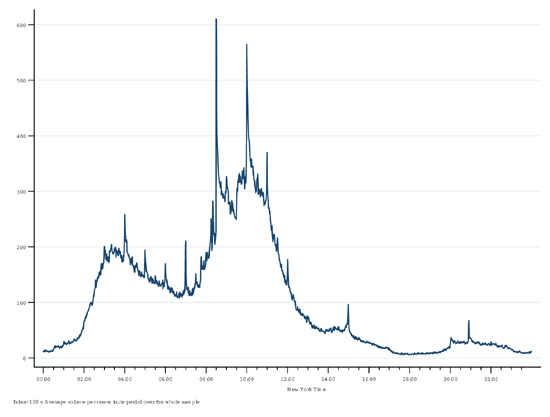
Figure 2. Plots of the Logged Daily Data

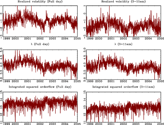
Figure 3. Plots of the 40-day moving average of the demeaned log-transformed realized volatility $\left ( RV_{t}\right )$, the estimated $\lambda _{t}s$, and the integrated squared orderflow $\left ( OF_{t}^{\left ( 2\right ) }\right )$

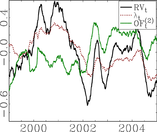
Figure 4. Plots of Realized Volatility and the Corresponding Regression Residuals

Figure 5. Auto-Correlograms of Realized Volatility and the Corresponding Regression Residuals

Figure 6. The Standardized Unconditional Distribution of the Actual and Fitted Values of the Log of Realized Volatility

Figure 7. Plots of the 40-day moving average of the demeaned log-transformed realized volatility $\left ( RV_{t}\right )$, and volume of trade $\left ( V_{t}\right )$

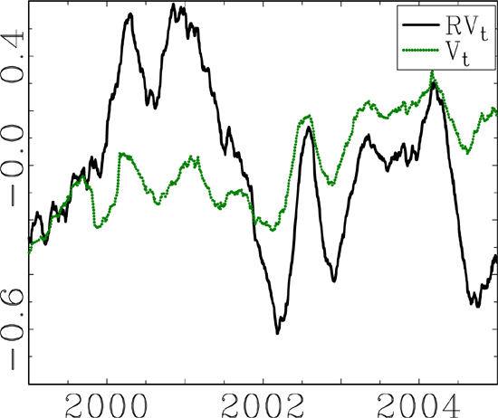
Footnotes

1.  We have benefitted from comments by David Bowman, Mark Carey, Frank Diebold, Jon Faust, Joe Gagnon, Dale Henderson, Lennart Hjalmarsson, Mico Loretan, Mark Seasholes, Clara Vega, Jon Wongswan, Jonathan Wright, Pär Österholm, and seminar participants at the Federal Reserve Board. The views presented in this paper are solely those of the authors and do not represent those of the Federal Reserve Board or its staff. Return to text

2.  Berger, Chaboud, and Hjalmarsson are with the Division of International Finance, Federal Reserve Board, Mail Stop 20, Washington, DC 20551, USA. Howorka is with EBS, 535 Madison Avenue, New York, NY 10022. Corresponding author: Erik Hjalmarrson. Tel.: +1-202-452-2436; fax: +1-202-263-4850; email: [email protected]. Return to text

3.  Another line of research has attempted to use the number of news stories released by financial wire services as measures of the rate of information arrival in the stock market, such as Mitchell and Mulherin (1994) and Berry and Howe (1994). This has met with very limited success, as the number of news stories explains only a small fraction of stock return volatility. Return to text

4.  In models relating volatility and volume there are indications that failure to account for the endogeneity of volume leads to biased inference. Lamoureux and Lastrapes (1990), for instance, find apparently strong evidence that volume can explain the GARCH effects in return volatility. However, in later work, Lamoureux and Lastrapes (1994) use a mixture model with a latent factor to relax the exogeneity assumption and find that this model cannot explain the persistence in volatility. The latter model is, however, fairly restrictive in nature, which makes it difficult to draw any strong conclusions regarding the causes of its failure. Return to text

5.  Bollerslev and Jubinski (1999) and Liesenfeld (2002) consider the long-memory in volatility and trading volume, although only Liesenfeld (2002) performs any formal tests of fractional cointegration; both articles find little or no support that volatility and trading volume share a common long-run component. Bandi and Perron (2004) use fractional cointegration to analyze the relationship between implied and realized volatility. Return to text

6.  EBS does not publish trading volume data per currency pair. To give a sense of an order of magnitude, average daily trading volume (the dollar amount traded) on EBS in euro-dollar in 2003, for instance, was well above that of the NYSE as a whole. Average daily trading volume on the NYSE in 2003 was about $40 billion. Traders on EBS can transact in amounts ranging from 1 to 999 million of the base currency. In practice, however, as large deals are routinely broken down, most transactions are for amounts of 1 to 5 million, and the average trade size varies little over time. As a result, there is a very high correlation between the trading volume in a given time period and and the number of transactions in that same period. Return to text

7.  In this market, by global convention, the value date changes at 17:00 New York time (whether or not it is Eastern Standard time or Eastern Daylight time), which therefore represents the official cutoff between two trading days. Return to text

8.  One of EBS's computer centers, located near the World Trade Center in New York, was temporarily disabled after the September 11 attack. Return to text

9.  These results are close to what Evans and Lyons (2002) report in their study of the impact of daily order flow on daily exchange rate returns. Return to text

10.  Empirical work conducted on the same dataset supports the conclusion that the $\lambda_{t}$ coefficients can be interpreted as the market sensitivity to new information. Berger et al. (2005, table 9) estimate a Hasbrouck-style (1991) VAR at the one-minute frequency. They report that order flow shocks account for about 40 percent of permanent exchange rate variation. Breaking the day into several intervals, they also show that order flow explains the largest share of exchange rate variation during the periods of highest global trading volume, including the times when most macroeconomic data are released. These results suggest that order flow is conveying information to the traders through the trading process and thus that the $\lambda_{t}$'s can reasonably be interpreted as capturing the market sensitivity to new information. Return to text

11.  In Kyle's (1985) analysis, $of_{t,i}$ represents unexpected orderflow, rather than total observed orderflow, which all the empirical results reported in this paper are based on. As a robustness check, we also constructed a proxy for unexpected orderflow by AR-filtering the observed orderflow. The results from the filtered data were very similar to those reported here for the total orderflow and are not shown in the paper. Return to text

12.  In the same vein, Andersen et al. (2004) study the time series properties of realized CAPM betas. Return to text

13.  In both of the two daily samples thus obtained, there are two days for which the estimated $\lambda_{t}$ is negative, although not statistically significantly different from zero. Interestingly, these are days when U.S. monthly payroll data were released, with large jumps in the exchange rate instantaneously associated with the data releases. Since negative values of $\lambda_{t}$ make little economic sense and prevent a log-transformation, we drop these rare days from our sample. The actual number of days used in each sample is thus $T=1487$. Return to text

14.  We use the estimator developed by Shimotsu (2004) that allows for an unknown mean in the data. In particular, following the results of Shimotsu (2004), if $x_{t}$, $t=1,...,T$ represent the data, the ELW estimator is applied to $x_{t}-\hat{\mu}\left( d\right)$ where $\hat{\mu }\left( d\right) =\omega\left( d\right) \bar{x}+\left( 1-\omega\left( d\right) \right) x_{1}$ , with $\omega\left( d\right) =1$ for $d\leq1/2$, $\omega\left( d\right) =0$ for $d\geq3/4$, $\omega\left( d\right) =\left( 1/2\right) \left[ 1+\cos\left( -2\pi+4\pi d\right) \right]$ for $1/2<d<3/4$, and $\bar{x}$ is the sample mean. Return to text

15.  The bandwidth restrictions given here, and below, are typically simplified versions of the exact restrictions given in the orginal papers. The rate restrictions provided here are meant to convey the primary intuition behind the choice of bandwidth and not a formal result. Return to text

16.  Hannan (1970) provides a textbook treatment on frequency domain methods and Engle (1974) gives an early economic application. Return to text

17.  The bandwidths used here for the estimation of $d$, and below in the NBLS and FMNBLS estimation, are all of the form $m=\left[ T^{\gamma }\right]$, for $\gamma=0.3,0.4,0.5,0.6$ and $0.7$. The highest frequencies included in the spectral analysis for these bandwidths correspond approximately to time-domain horizons of 185, 80, 40, 20, and 10 days, respectively. Return to text

18.  The NBLS estimates are asymptotically normal under the stronger assumptions that $d+d_{u}<0.5$, and that the long-run correlation between the regressors and the error terms is zero; that is the regressors can be endogenous in the short run (the higher frequencies in the spectral domain) but not in the long run (the frequencies close to zero); Christensen and Nielsen (2004). Whereas the former condition is likely to hold, there is no a priori reason to assume that the latter one holds. Return to text

19.  Since the $\lambda _{t}s$ are generated regressors, this may affect the econometric analysis. However, we conjecture that the strength of the fractional cointegrating relationship dominates the potential effects arising from the use of a generated regressor, and that, at least asymptotically, there should be no difference between using the true values and the generated values of the $\lambda _{t}s$. Monte Carlo simulations, not reported in the paper, show that there is little or no difference between the estimates resulting from the use of the true $\lambda _{t}s$ or the generated ones. Return to text

20.  There are 23 days where either the one minute residuals or the five minute residuals are greater than $0.75$ (which is approximately equal to two standard deviations). On 16 of these days there are US macroannouncements and on an additional five more of these days there are ECB or German macro announcements. In summary, 21 of the 23 of the outlier days are thus days with macro announcements. Return to text

21.  We made one attempt at directly measuring the arrival of information, using the number of international Dow Jones news stories per day. The data collected was the total number of daily Dow Jones international news wire stories (collected from Factiva) excluding repeated stories, fixed market updates and sports stories (a fixed market update says, for instance, that the euro-dollar exchange rate was 1.21 at 1:00 GMT). We choose this flexible categorization because other than sports, all the other subcategories under Dow Jones international seemed as if they could be relevant. Also, the EBS terminal provides users with a real time Dow Jones news feed so this series was the natural choice to try. We regressed realized volatility onto the Dow Jones news stories variable by itself, as well as jointly with the $\lambda _{t}s$. The lattter multiple regression was motivated by the finding that there was little evidence that squared orderflow in itself could explain volatility persistence, and to the extent that both squared orderflow and the Dow Jones stories proxy for some information arrival we might expect similar results here. The regression results, which are omitted here, showed no evidence that the Dow Jones variable could explain any of the persistence in volatility, either by itself or jointly with the $\lambda _{t}s$. Return to text

22.  In the stock-market literature, it is common to use the number of transactions, rather than the volume of trade, as a measure of market activity. We therefore performed the same analysis as just described, but with volume replaced by the number of transactions. Overall, the results were similar, but perhaps a bit weaker, when using the number of transactions and the results are not reported here for brevity. As stated previously, in the electronic interdealer foreign exchange data that we study, the majority of trades is for amounts between 1 and 5 million euros, as large orders are routinely broken up before execution. As a result, the average trade size shows little time variation, and the number of transactions and the trading volume show a high degree of correlation. Return to text

23.  As pointed out above, separate $d-$parameters are estimated for each variable and these distinct estimates are used in forming the FMNBLS estimator. Return to text

This version is optimized for use by screen readers. A printable pdf version is available.

Home | Economic research and data | Publications and education resources
Accessibility | Contact us
Last update: May 31, 2006