Skip to: [Printable Version (PDF)]

Board of Governors of the Federal Reserve System
International Finance Discussion Papers
Number 880, October 2006 --- Screen Reader Version*

Optimal Fiscal and Monetary Policy When Money is Essential^*

S. Borağan Aruoba^†, University of Maryland
Sanjay K. Chugh^‡, Federal Reserve Board

[The PDF document is dated "October 6, 2006."]

NOTE: International Finance Discussion Papers are preliminary materials circulated to stimulate discussion and critical comment. References in publications to International Finance Discussion Papers (other than an acknowledgment that the writer has had access to unpublished material) should be cleared with the author or authors. Recent IFDPs are available on the Web at http://www.federalreserve.gov/pubs/ifdp/. This paper can be downloaded without charge from the Social Science Research Network electronic library at http://www.ssrn.com/.

Abstract:

We study optimal fiscal and monetary policy in an environment where explicit frictions give rise to valued money, making money essential in the sense that it expands the set of feasible trades. Our main results are in stark contrast to the prescriptions of earlier flexible-price Ramsey models. Two especially important findings emerge from our work: the Friedman Rule is typically not optimal and inflation is stable over time. Inflation is not a substitute instrument for a missing tax, as is sometimes the case in standard Ramsey models. Rather, the inflation tax is exactly the right tax to use because the use of money has a rent associated with it. Regarding the optimal dynamic policy, realized (ex-post) inflation is quite stable over time, in contrast to the very volatile ex-post inflation rates that arise in standard flexible-price Ramsey models. We also find that because capital is underaccumulated, optimal policy includes a subsidy on capital income. Taken together, these findings turn conventional wisdom from traditional Ramsey monetary models on its head.

Keywords: micro-founded models of money, Friedman Rule, inflation stability

JEL classification: E13, E52, E62, E63

*  The views in this paper are solely the responsibility of the authors and should not be interpreted as reflecting the views of the Board of Governors of the Federal Reserve System or of any other person associated with the Federal Reserve System. Return to text

  †E-mail address: [email protected]. Return to text

  ‡E-mail address: [email protected] Return to text

Contents

• 1  Introduction
• 2  Basic Model
• 2.1  Government
• 2.2  Households
• 2.2.1  Household CM Problem
• 2.2.2  Household DM Problem
• 2.2.3  Bargaining Version
• 2.2.4  Price-Taking
• 2.2.5  Solution to Household Problem
• 2.3  Firms
• 2.4  Equilibrium

• 3  Ramsey Problem in Basic Model
• 4  Optimal Policy in Basic Model
• 4.1  Optimal Positive Nominal Interest Rate when theta = 1
• 4.2  Numerical Results
• 4.2.1  Solution Strategy and Parameterization
• 4.2.2  Ramsey Steady-State
• 4.2.3  Ramsey Dynamics

• 5  Model with Capital
• 5.1  Production
• 5.2  Households
• 5.2.1  Household DM Problem - Bargaining
• 5.2.2  Household DM Problem - Price-Taking
• 5.3  Government
• 5.4  Equilibrium
• 5.4.1  Bargaining
• 5.4.2  Price-Taking

• 6  Ramsey Problem in Model with Capital
• 7  Optimal Policy in Model with Capital
• 7.1  Optimal Positive Nominal Interest Rate
• 7.2  Numerical Results for the Bargaining World
• 7.2.1  Solution Strategy and Parameterization
• 7.2.2  Ramsey Steady-State
• 7.2.3  Ramsey Dynamics
• 8  Conclusion
• A  The Ramsey Problem in Basic Model
• A.1  Proof of Proposition 1
• A.2  The Solution to the Ramsey Problem
• B  Alternative Instruments in the DM in Basic Model
• C  The Ramsey Problem in Model with Capital
• C.1  Proof of Proposition 3
• C.2  The Solution to the Ramsey Problem

1  Introduction

Monetary theory has made important advances of late, ones that enable researchers interested in applied policy questions to consider explicit frictions that give rise to valued money. In this paper, we build on the works of Lagos and Wright (2005) and Aruoba, Waller, and Wright (2006); in these new environments, we study optimal fiscal and monetary policy, following the tradition of Lucas and Stokey (1983) and Chari, Christiano, and Kehoe (1991). Two important findings emerge from our work, both of which are opposite those of earlier flexible-price Ramsey monetary models: the Friedman Rule is typically not optimal and inflation is stable over time. Our results thus turn conventional wisdom from traditional Ramsey models on its head.

The contribution of Lagos and Wright (2005) and Aruoba, Waller, and Wright (2006) -- hereafter, LW and AWW, respectively -- is to integrate search-based monetary theory, in the spirit of Kiyotaki and Wright (1989, 1993), with standard dynamic general equilibrium macroeconomics. This integration makes the study of policy questions much easier and potentially more relevant than in earlier search-based models. However, these models have been criticized on two grounds. First, they superficially resemble standard cash-in-advance (CIA) or money-in-the-utility-function (MIU) models, raising some question about whether they really are any deeper than reduced-form models of money. This point has been raised by, among others, Howitt (2003). Second, until now, the policy questions addressed in these new models have been largely confined to the deterministic welfare costs of inflation. When parameterized to seem as close as possible to standard CIA and MIU models, the quantitative answers they have yielded to this question are similar to those obtained with CIA and MIU models, further adding to the sense that these new models simply re-invent CIA or MIU. In this paper, we ask a different policy-relevant question in these new models, and even when we parameterize the model to look very similar to standard applied models of money, we reach conclusions very different from those reached by Chari, Christiano, and Kehoe (1991) and others using typical CIA and MIU frameworks. Our results thus show that the answers to policy questions may indeed be very different once monetary frictions are treated seriously.

We study the canonical Ramsey problem of optimal fiscal and monetary policy using the LW and AWW models. Our first main finding is that the optimal nominal interest rate is typically positive. This optimal deviation from the Friedman Rule is not because the inflation tax acts as a substitute instrument for a missing tax, as is sometimes the case in Ramsey models. Rather, the inflation tax is exactly the right tax for the government to use when money is essential in Kocherlakota's (1998) sense that it expands the set of feasible trades. Specifically, without money, trade can only occur if there is a double coincidence of wants, whereas money allows trade to occur with only a single coincidence of wants. Money is thus a special object in this class of models and therefore has a rent associated with it. Households in our economy require the benefit of holding money to be strictly positive to be induced to hold it. This benefit is realized only when the household is a buyer in a bilateral match in the form of buyer's surplus, and it is this surplus that we interpret as the rent associated with holding money. It is well-known from Ramsey theory that it is optimal to tax rents. The most direct way to tax rents accruing to money is through inflation, hence the Friedman Rule is not optimal. Interestingly, Kocherlakota (2005) conjectured that the Friedman Rule may not be optimal in a Ramsey problem in search-based models. Our results show his conjecture is correct.

Deviations from the Friedman Rule have also been obtained in other modern Ramsey models. For example, Schmitt-Grohe and Uribe (2004a) show that a positive nominal interest rate can tax producers' monopoly profits, and Chugh (2006b) shows it can tax monopolistic labor suppliers' rents.¹ Both of these results, however, are examples of the Ramsey planner using a positive nominal interest rate to indirectly tax some rent. One may wonder whether alternative tax instruments in our model could tax the money rent. To investigate this, we introduce a sales tax on goods whose purchase can only be achieved with money. It turns out that adding this seemingly natural instrument does not admit a Ramsey equilibrium in which the Friedman Rule is optimal. Thus, if there does exist another tax instrument besides the inflation tax that can seize the money rent, it is not an obvious one.

Our second main finding is that realized (ex-post) inflation is quite stable over time in the face of shocks, which is in contrast to the very volatile ex-post inflation rates that Chari, Christiano, and Kehoe (1991) -- hereafter, CCK -- find. Inflation volatility is high in CCK and the related literature because surprise movements in the price level allow the government to synthesize real state-contingent debt payments from nominally risk-free government bonds, without distorting the relative prices of consumption goods. The government then need not change other, distortionary, tax rates much in response to shocks. In our model, in contrast, real activity is distorted by ex-post inflation because inflation affects relative prices of goods, in a way that a flexible-price CIA or MIU model cannot articulate. The welfare cost of this relative-price distortion dominates the insurance value of generating state-contingent debt in our model, rendering inflation very stable. The frictions underlying monetary trade thus provide novel justification for the optimality of inflation stability, a prescription that resonates with most central bankers. This result also echos the long-standing idea in monetary economics that inflation variability is undesirable because it induces relative price shifts.

Finally, when we allow for capital accumulation, the optimal policy includes a subsidy on capital income. Both the frictions inherent in bilateral trade in our model as well as the deviation from the Friedman Rule tend to depress capital accumulation compared to its efficient level. A capital subsidy somewhat alleviates this problem.

An important technical advantage of the LW and AWW frameworks is that the distribution of money-holdings across agents is simple to track: it simply collapses periodically to a point. At the expense of a heavier computational burden, one may want to think about optimal fiscal and monetary policy when this distribution is non-trivial. Once one goes down that route, an interesting taxation framework to apply may be the Mirrleesian one, in which idiosyncratic shocks and private information become important considerations in shaping optimal policy. However, because even the simpler step of characterizing the Ramsey-optimal policy, which assumes a representative agent, has not been studied in this class of models, we think it makes sense to begin here.

The rest of the paper is organized as follows. Section 2 lays out the baseline LW model in which we first study optimal policy. Most of the important results and intuition emerge in this basic model. Section 3 presents the Ramsey problem for the basic model. In Section 4, we characterize and discuss the optimal policy in the basic model; we present in Section 4.1 a proof for a particularly important version of the model that the Friedman Rule is not optimal and in Section 4.2 the dynamic Ramsey allocations and policy that demonstrate optimal inflation stability. In Sections 5 and 6, we extend the Ramsey problem to the AWW model, and Section 7 shows that the main results carry over from the basic model virtually unchanged. Section 8 summarizes and offers ideas for future work.

2  Basic Model

We begin by establishing our main results in a version of the LW model. In this model, the agents in the economy participate in a centralized market (CM) where they trade general consumption goods and assets with the market and in a decentralized market (DM) where they trade specialized consumption goods bilaterally. To enhance comparability with the benchmark cash-credit environment used by CCK, we alter slightly the timing of markets in the original LW model. Specifically, in our version, the CM is the first market in a given period, followed by the DM. We make this alteration because we would like asset markets (which in the LW model meet in the CM) to convene in any period before goods markets (in particular, before goods markets in which money must be used for transactions), which is the timing assumed by CCK. However, we do not see how any of our results depend on the temporal ordering of markets within a period. We proceed by describing the activities of the government, households, and firms in our model.

2.1  Government

Government consumption is assumed to be composed entirely of goods produced in the CM. In nominal terms, the flow budget constraint of the government is

$$M_{t} + B_{t} + P_{t} w_{t} \tau^{h}_{t} H_{t} = P_{t} G_{t} + M_{t-1} + R_{t-1}B_{t-1},$$ (1)

which states that the government has three sources of revenues to pay for its consumption: labor income tax revenues, nominal money creation, and nominal debt issuance. The notation is standard: $M_{t}$ denotes nominal money outstanding at the end of period $t$, $B_{t}$ is nominally risk-free government debt outstanding at the end of period $t$, $R_{t}$ is the gross nominal interest rate on bonds, $\tau^{h}_{t}$ is a proportional labor income tax on aggregate hours worked $H_{t}$ in the CM, $P_{t}$ is the nominal price level in the CM, and $w_{t}$ is the real wage in the CM. The nominal return $R_{t}$ is known at the time $B_{t}$ is issued and paid in the CM of period $t+1$. We assume that bonds are simply book entries with no tangible proof that one can carry around.

2.2  Households

Households periodically transact in markets for general goods and assets (the CM) and in markets for specialized goods (the DM). In the DM, money is essential in the sense that transactions there are infeasible without money.² In the CM, because markets are Walrasian trades can proceed with or without money. We describe first the timing of events in a given period and then present the household's CM and DM problems.

Events unfold for a household in a given period $t$ as follows:

• The household begins the CM with portfolio $m_{t-1}$ and $b_{t-1}.$
• The uncertainty for the current period is resolved, and the household observes government consumption $G_{t}$ and the level of technology $Z_{t}$. We denote the aggregate state collectively by $S_{t}$.
• The household receives the receipts from bond holdings, $R_{t-1}b_{t-1}$.
• The household chooses its CM consumption $x_{t}$, labor supply $h_{t}$, portfolio $(m_{t},b_{t})$ and pays the labor income tax.
• The household enters the DM with $m_{t}$.
• Depending on the household's trade in the DM, it exits the DM with $m_{t}-d_{t},$ $m_{t}+d_{t}$, or $m_{t}$ money holdings, where $d_{t}$ is the buyer's payment in bilateral trade.

2.2.1  Household CM Problem

For a household that enters the CM with money holdings $m_{t-1}$ and bond holdings $b_{t-1}$, the CM problem is

$$W_{t}\left( m_{t-1}, b_{t-1}, S_{t}\right) = \max_{x_{t},h_{t},m_{t},b_{t}} \left\{ U(x_{t}) - Ah_{t} + V_{t}(m_{t} ,b_{t},S_{t}) \right\}$$ (2)

subject to

$$P_{t} x_{t} + m_{t} + b_{t} = P_{t} w_{t} (1-\tau_{t} ^{h})h_{t} + m_{t-1} + R_{t-1} b_{t-1},$$ (3)

where $W_{t}(.)$ denotes the value of entering the CM and $V_{t}(.)$ denotes the value of entering the DM that convenes after the CM in period $t$. Centralized market consumption is $x_{t}$, and the household's hours worked in the CM is $h_{t}$. Note that instantaneous utility in the CM is separable and linear in labor; it is this quasi-linearity in preferences that allows the LW model to be tractable, as it guarantees a degenerate distribution of money holdings across households after every meeting of the CM.

Eliminating $h$ in the objective function using the budget constraint, the first-order conditions with respect to $x_{t}$, $m_{t}$, and $b_{t}$ are

$$U^{\prime}(x_{t}) = \frac{A}{w_{t}(1-\tau_{t}^{h})},$$ (4)

$$\frac{A}{P_{t} w_{t} (1-\tau_{t}^{h})} = V_{m,t} (m_{t} ,b_{t},S_{t}),$$ (5)

$$\frac{A}{P_{t} w_{t} (1-\tau_{t}^{h})} = V_{b,t} (m_{t} ,b_{t},S_{t}),$$ (6)

familiar from LW. These optimality conditions imply the usual LW results about degeneracy of asset holdings $(m_{t},b_{t})$ across households because they are independent of $(m_{t-1},b_{t-1})$.³ All households choose the same portfolio at the end of the CM regardless of the portfolio they entered the market with. Thus, the LW result of degeneracy of money holdings readily extends to bond holdings as well. Moreover, we have standard envelope conditions

$$W_{m,t}(m_{t-1},b_{t-1},S_{t}) = \frac{A}{P_{t}w_{t}(1-\tau_{t}^{h})},$$ (7)

$$W_{b,t}(m_{t-1},b_{t-1},S_{t}) = \frac{A R_{t-1}}{P_{t}w_{t}(1-\tau_{t}^{h})},$$ (8)

which show $W_{t}(.)$ is linear in its arguments.

2.2.2  Household DM Problem

Now we turn to the household's DM problem. Knowing that the distribution of money holdings is degenerate in equilibrium, we will, for notational simplicity, write the household DM problem assuming that when it meets a trading partner, the trading partner has equilibrium money holdings $M_{t}$; this allows us to conserve on integrating over all possible money holdings of trading partners that a given household could meet. With probability $\sigma$, the household is a buyer in the DM; with probability $\sigma$, the household is a seller in the DM; and with probability $1-2\sigma$, the household does not participate in the DM and continues to the CM of the next period without transacting.⁴Buyers consume $q$ in the DM, experiencing utility $u(q)$; sellers produce $q$ in the DM, experiencing disutility, which can be interpreted as the cost of production, $c(q,Z)$, where $c_{Z} < 0$. We assume throughout our basic model that $c(q,Z)=q/Z$.⁵

We can write the problem of a household that enters the DM with portfolio $(m_{t},b_{t})$ as

$$V_{t}(m_{t},b_{t},S_{t}) = \sigma\left\{ u\left[ q\left( m_{t}, M_{t}, S_{t}\right) \right] + \beta E_{t} W_{t+1}\left[ m_{t}- d(m_{t},M_{t},S_{t}), b_{t}, S_{t+1} \right] \right\}$$ (9)

$$+ \sigma\left\{ -c\left[ q\left( M_{t},m_{t},S_{t}\right) , Z_{t}\right] + \beta E_{t} W_{t+1}\left[ m_{t} + d(M_{t},m_{t},S_{t}), b_{t}, S_{t+1} \right] \right\}$$ (10)

$$+ (1-2\sigma) \beta E_{t} W_{t+1}\left( m_{t},b_{t},S_{t+1}\right) .$$ (11)

The quantity $q(m_{bt},m_{st},S_{t})$ is the quantity produced and exchanged in a bilateral meeting in the DM, where $m_{b}$ denotes the money holdings of the buyer, $m_{s}$ denotes the money holdings of the seller, and $d(m_{b},m_{st},S_{t})$ is the amount of money that changes hands. We refer to $[q(.), d(.)]$ as the terms of trade in a single-coincidence meeting. Note that due to the nature of the bonds, neither the buyer's nor the seller's bond holdings will matter for $q$ and $d$.

In the DM, we must specify the protocol by which the price and quantity in any bilateral trade are determined -- that is, we must define the structure by which the terms of trade are determined. The two main alternatives in the literature are Nash bargaining and price-taking. We describe the bargaining version in detail. It turns out -- see Rocheteau and Wright (2005) -- that price-taking in the basic model amounts to a simple parameter restriction in the bargaining version.

2.2.3  Bargaining Version

Denoting the portfolio of the buyer by $(m_{t},b_{t})$, that of the seller by $(\tilde{m}_{t}, \tilde{b}_{t})$, and the buyer's bargaining power by $\theta$, the generalized Nash bargaining problem is

$${\scriptsize\max_{q_{t},d_{t}}\left[ u(q_{t}) + \beta E_{t} W_{t+1}\left( m_{t}-d_{t}, b_{t},S_{t+1}\right) - \beta E_{t} W_{t+1}\left( m_{t} ,b_{t},S_{t+1}\right) \right] ^{\theta}}$$ (12)

$$\times\left[ -c(q_{t},Z_{t}) +\beta E_{t} W_{t+1}\left( \tilde{m}_{t} +d_{t},\tilde{b}_{t},S_{t+1}\right) - \beta E_{t} W_{t+1}\left( \tilde {m}_{t},\tilde{b}_{t},S_{t+1}\right) \right] ^{1-\theta}$$ (13)

subject to

$$d_{t} \leq m_{t}.$$ (14)

where the constraint is simply a feasibility condition stating the buyer cannot spend more than he has and the threat points are the values of continuing on to the next CM in period $t+1$. Using the envelope conditions from above (in particular, the implied linearity of the function $W_{t}(.)$), the bargaining problem can be written more conveniently as

$$\max_{q_{t},d_{t}} \left\{ u(q_{t}) - \beta d_{t} E_{t} \left[ \frac{A}{P_{t+1} w_{t+1} (1-\tau^{h}_{t+1})} \right] \right\} ^{\theta} \left\{ -c(q_{t}, Z_{t}) + \beta d_{t} E_{t} \left[ \frac {A}{P_{t+1} w_{t+1} (1-\tau^{h}_{t+1})}\right] \right\} ^{1-\theta}$$ (15)

subject to

$$d_{t} \leq m_{t}.$$ (16)

We define $\chi_{t} \equiv E_{t} \left[ A/\{P_{t+1} w_{t+1} (1-\tau^{h} _{t+1})\} \right]$ which can be interpreted as the marginal utility of consumption of $t+1$ CM goods that are worth one unit of money using (4). Then, the Kuhn-Tucker conditions, which are necessary and sufficient, for the bargaining problem are

$$\frac{\theta u^{\prime}(q_{t}) }{u(q_{t}) - \beta\chi_{t} d_{t}} - \frac{(1-\theta) c_{q}(q_{t},Z_{t})}{-c(q_{t},Z_{t}) + \beta\chi_{t} d_{t} } = 0,$$ (17)

$$-\frac{\theta\beta\chi_{t} }{u(q_{t}) - \beta\chi_{t} d_{t}} +\frac{(1-\theta) \beta\chi_{t} }{-c(q_{t},Z_{t}) + \beta\chi_{t} d_{t}} - \lambda_{t} = 0,$$ (18)

$$\lambda_{t}(m_{t} - d_{t}) = 0,$$ (19)

where $\lambda_{t}$ is the multiplier associated with the constraint. If $\lambda_{t}=0$, the first two conditions yield $u^{\prime}(q_{t})=c_{q} (q_{t},Z_{t})$, which defines the efficient quantity $q_{t}=q^{*}$, and $d_{t}=m_{t}^{*}$, which can be solved using the second equation.

If $\lambda_{t}>0$, the solution will have $d_{t}=m_{t}$, meaning the buyer spends all his money in a bilateral meeting. Using the first condition, the quantity produced and traded will solve

$$\beta\chi_{t} m_{t} = g(q_{t},Z_{t}),$$ (20)

where

$$g(q,Z) \equiv\frac{ \theta c(q,Z) u^{\prime}(q) + (1-\theta)u(q)c_{q}(q,Z) }{ \theta u^{\prime}(q) + (1-\theta) c_{q}(q,Z) }$$ (21)

as in LW. In equilibrium, $\lambda_{t}>0$, which can be shown using a similar argument to the one in LW. Also, note that because the expectation in $\chi_{t}$ is taken with respect to $S_{t}$, we denote the bargaining problem outcomes as $q(m_{t},S_{t})$ and $d(m_{t},S_{t})$, where the first argument is understood to be the money holdings of the buyer.

Substituting this solution into the DM problem (9) and using the envelope conditions for $W_{t}(.)$, we get

$$V_{t}(m_{t},b_{t},S_{t}) = \sigma\left\{ u\left[ q_{t}\left( m_{t} ,S_{t}\right) \right] -c\left[ q\left( M_{t},S_{t}\right) , Z_{t} \right] - \beta\chi_{t} m_{t} + \beta\chi_{t} M_{t} \right\} + \beta E_{t}W_{t+1}\left( m_{t},b_{t},S_{t+1}\right) .$$ (22)

The relevant envelope conditions for $V_{t}(.)$ are

$$V_{m,t}\left( m_{t},b_{t},S_{t}\right) = \sigma\left\{ u^{\prime}\left[ q_{t}\left( m_{t},S_{t}\right) \right] \frac{\partial q_{t}\left( m_{t},S_{t}\right) }{\partial m_{t}} - \beta\chi_{t} \right\} + \beta\chi_{t},$$ (23)

$$V_{b_{t},t}\left( m_{t},b_{t},S_{t}\right) = \beta R_{t} \chi_{t}.$$ (24)

Finally, noting

$$\frac{\partial q_{t}}{\partial m_{t}} = \frac{\beta\chi_{t} }{g_{q}(q_{t},Z_{t})}$$ (25)

from (20), (23) simplifies to

$$V_{m,t}\left( m_{t},b_{t},S_{t}\right) = \beta \chi_{t} \left[ \sigma\frac{u^{\prime}(q)}{g_{q}(q,Z)} + 1 - \sigma\right] .$$ (26)

2.2.4  Price-Taking

Although bargaining has been used almost exclusively as the pricing scheme in bilateral meetings in this class of models, more ``competitive'' pricing schemes have been used recently, as well. In addition to being closer to mainstream macroeconomics, competitive pricing eliminates the holdup problems inherent in bargaining. In the basic model, competitive pricing in the DM amounts to sellers and buyers solving their respective supply and demand problems taking the price as given; the market-clearing price is determined in equilibrium. Based on the results of LW and Rocheteau and Wright (2005), it follows that the price-taking version of our model is the same as the bargaining version with $\theta = 1$.

2.2.5  Solution to Household Problem

For the bargaining version we obtain the conditions that solve the household's problem as follows. First, combining the household's CM optimality conditions (4)-(6) with the envelope conditions (23) and (24) gives us:

$$U^{\prime}(x_{t}) = \frac{A}{(1-\tau^{h}_{t})w_{t}},$$ (27)

$$\frac{A}{P_{t}w_{t}(1-\tau_{t}^{h})} = \beta\chi_{t} \left[ \sigma\frac{u^{\prime}(q)}{g_{q}(q,Z)} + 1 - \sigma\right] ,$$ (28)

$$\frac{A}{Pw(1-\tau^{h})} = \beta R_{t} \chi_{t}.$$ (29)

Using (27) and the definition of $\chi_{t}$, we get

$$\chi_{t} = E_{t} \left[ \frac{U^{\prime}(x_{t+1})}{P_{t+1}} \right] ,$$ (30)

which we can use to express (28) and (29) as

$$\frac{U^{\prime}(x_{t})}{P_{t}} = \beta\left[ \sigma \frac{u^{\prime}(q_{t})}{g_{q}(q_{t},Z_{t})} + 1 - \sigma\right] E_{t} \left[ \frac{U^{\prime}(x_{t+1})}{P_{t+1}}\right] ,$$ (31)

$$\frac{U^{\prime}(x_{t})}{P_{t}} = \beta R_{t} E_{t}\left[ \frac{U^{\prime}(x_{t+1})}{P_{t+1}}\right] .$$ (32)

We will refer to these last two equations as the household's first-order conditions with respect to money and bonds, respectively, in analogy with a standard cash/credit CCK type of model. Note that they imply a Fisher-like condition,

$$R_{t} = \sigma\frac{u^{\prime}(q_{t})}{g_{q}(q_{t},Z_{t})} + 1 - \sigma,$$ (33)

linking the returns on money and bonds.

Rewriting condition (33) slightly, we have

$$i_{t} = \sigma\left[ \frac{u^{\prime}(q_{t})}{g_{q}(q_{t} ,Z_{t})} - 1 \right] ,$$ (34)

where the left hand side, $i \equiv R - 1$, is the cost of holding money (the net nominal interest rate) and the right hand side is the benefit of holding money. We note that the right-hand-side of (34) will play an important role in shaping the Ramsey allocations and hence the optimal policy; we defer discussion and intuition regarding it until we present the Ramsey problem in Section 3, in which we will see it in the context of the complete Ramsey problem and will be able to easily compare it to the benchmark Ramsey problems in Lucas and Stokey (1983) and CCK.

To finally state the solution of the household problem: given sequences $\{S_{t}, P_{t}, w_{t}, \tau^{h}_{t}, R_{t}\}$, initial condition $(M_{0}, B_{0})$, and appropriate transversality conditions, the solution to the household's problem is processes $\{q_{t}, M_{t}, B_{t}, x_{t}, h_{t} \}_{t=0}^{\infty}$ satisfying conditions (3), (20 ), (27), (31), and (33).

2.3  Firms

In the CM, a representative firm hires labor in a competitive labor market and operates the linear production technology $Y_{t} = Z_{t} H_{t}$. Profit-maximization therefore implies the wage is $w_{t} = Z_{t}$ in equilibrium.

2.4  Equilibrium

Imposing equilibrium ( $m_{t}=M_{t}$, $x_{t}=X_{t}$, etc.) and combining the firms' and households' optimality conditions, we can define the equilibrium as follows. Given policy variables $\{\tau^{h}_{t}, R_{t}\}_{t=0}^{\infty}$, the technology realization $\{Z_{t}\}_{t=0}^{\infty}$, the government spending realization $\{G_{t}\}_{t=0}^{\infty}$, and initial condition $(M_{0}, B_{0})$, equilibrium is a set of processes $\{q_{t}, B_{t}, M_{t}, X_{t}, H_{t}, P_{t}\}_{t=0}^{\infty}$ satisfying

$$U^{\prime}(X_{t}) = \frac{A}{(1-\tau_{t}^{h})Z_{t} },$$ (35)

$$\beta M_{t} E_{t}\left[ \frac{U^{\prime}(X_{t+1} )}{P_{t+1}}\right] = g(q_{t},Z_{t}),$$ (36)

$$\frac{U^{\prime}(X_{t})}{P_{t}} = \beta\left[ \sigma\frac{u^{\prime}(q_{t})}{g_{q}(q_{t},Z_{t})} + 1 - \sigma\right] E_{t} \left[ \frac{U^{\prime}(X_{t+1})}{P_{t+1}}\right] ,$$ (37)

$$R_{t} = \sigma\frac{u^{\prime}(q_{t})}{g_{q}(q_{t},Z_{t})} + 1 - \sigma,$$ (38)

$$X_{t} + G_{t} = Z_{t} H_{t},$$ (39)

$$B_{t} + M_{t} + P_{t} G_{t} = R_{t-1} B_{t-1} + M_{t-1} + P_{t} Z_{t} \tau_{t}^{h} H_{t}.$$ (40)

For the Ramsey problem, it will be useful to combine (36) and (37) and rearrange for real money balances,

$$\frac{M_{t}}{P_{t}} = \frac{g(q_{t} ,Z_{t}) }{U^{\prime}(X_{t})} \left[ \sigma\frac{u^{\prime}(q_{t})} {g_{q}(q_{t},Z_{t})} + 1 - \sigma\right] .$$ (41)

Furthermore, in any monetary equilibrium, $R_{t} \geq1$ because otherwise households could earn unbounded profits by selling bonds and buying money. We represent this restriction in terms of allocations using (38) as

$$\sigma\left( \frac{u^{\prime}(q_{t})}{g_{q}(q_{t},Z_{t})} - 1 \right) \geq0.$$ (42)

3  Ramsey Problem in Basic Model

As is common in the Ramsey literature, we adopt the primal approach and cast the Ramsey problem as that of a planner that chooses allocations subject to feasibility and the need to raise exogenous government revenue, making sure the resulting allocations are implementable as a monetary equilibrium. We prove the following in Appendix A.1:

Proposition 1   The allocations in a monetary equilibrium satisfy (39), (42), and the present-value implementability constraint (PVIC),

$$E_{0} \sum_{t=0}^{\infty} \beta^{t} \left[ U^{\prime} (X_{t}) X_{t} - A H_{t} + \sigma g(q_{t},Z_{t}) \left( \frac{u^{\prime} (q_{t})}{g_{q}(q_{t},Z_{t})} - 1\right) \right] = U^{\prime}(X_{0}) \left[ \frac{M_{-1} + R_{-1} B_{-1}}{P_{0}} \right] .$$ (43)

In textbook Ramsey problems, implementability constraints typically take the form
$E_{0} \sum_{t} \beta^{t} \sum_{i} U_{i}(x_{1t},...,x_{Nt}) x_{it} = a_{0}$ , where $\{x_{it}\}_{i=1}^{N}$ is the set of $N$ goods the agent consumes at time $t$.⁶ At first glance, (43) does not seem to conform to this general form because the term related to the DM, $\sigma g(q_{t},Z_{t}) ( u^{\prime}(q_{t})/g^{\prime}(q_{t}) - 1 )$ does not look like marginal utility of a good times the quantity of that good. However, this term does indeed have such an interpretation; we can show that the term in the PVIC is simply the product of money balances and its marginal utility.

To see this, note that from the bargaining problem and (20), $S_{b}(q)\equiv u(q)-g(q,Z)$ is the surplus of the buyer and therefore $S^{\prime}_{b}(q)\equiv u^{\prime}(q)-g_{q}(q,Z)$ is the marginal surplus of the buyer. Moreover, money has no use in the DM unless the household is a buyer, which occurs with probability $\sigma$. Thus, the marginal utility of money can be expressed as $\sigma S^{\prime}_{b}(q) \partial q / \partial m$. From (20) and (25), we have $m = g(q,Z)/\beta\chi$ and $\partial q / \partial m = \beta\chi/ g_{q}(q,Z)$. Combining these, we obtain the third term under the summation in the PVIC. With this interpreration, one may argue that our model lolks like a MIU model, which would have a term $m U_{m}$ in the PVIC. In our context, though, the marginal utility of money is linked to the fundamentals of the economy -- allocations and technology -- and it is not an arbitrary function.

If $\sigma=0$, the DM shuts down and our PVIC collapses to the usual CCK PVIC in a real model. That is, the model collapses not to the CCK monetary (cash-credit) economy, but to a purely real model. This is a manifestation of the ``dichotomy" result the LW model displays that Aruoba and Wright (2003) pointed out. The inflation rate in the LW model does not affect CM allocations at all.⁷

Because we restrict attention to only monetary equilibria, we require that the Ramsey allocations satisfy restriction (42), which we refer to as the zero-lower-bound (ZLB) constraint. CCK show that in their model, the ZLB constraint always holds with equality under the solution of the Ramsey problem obtained by dropping the ZLB constraint; in other words, in the CCK model the Friedman Rule ($R_{t} = 1$) can be shown analytically to always be the optimal policy. Thus, in the CCK model it turns out the ZLB constraint is redundant regardless of the parameterization of the model. This is not the case in general in our model and thus we need to impose it. As a technical point, note that the ZLB constraint is an inequality constraint. Thus, when solving for the dynamics of the model, we must employ a nonlinear global numerical approximation to handle the occasionally binding constraint. In practice, though, for a very important parameterization of interest of the model, it turns out that the ZLB constraint can be shown to be slack -- in fact, that it is always satisfied with strict inequality. We discuss this further below, and it is one of our main results.

We assume the Ramsey planner is able to commit at time zero to a policy for $t \geq1$. We thus sidestep here the potentially interesting issue of time-inconsistency in this model. The Ramsey problem is thus to choose $\{X_{t}, H_{t}, q_{t}\}$ to maximize

$$E_{0} \sum_{t=0}^{\infty} \beta^{t} \left\{ U(X_{t}) - A H_{t} + \sigma\left[ u(q_{t})-c(q_{t},Z_{t})\right] \right\}$$ (44)

subject to the resource constraint

$$X_{t} + G_{t} = Z_{t} H_{t},$$ (45)

the PVIC (43), and the ZLB constraint (42), taking as given $\{G_{t}, Z_{t}\}$. In Appendix A.2, we list the conditions that characterize the solution to this problem, along with the conditions that allow us to construct the policies and prices that support the Ramsey allocation. Thus, as we already noted, our approach is a straightforward application of Ramsey theory.

4  Optimal Policy in Basic Model

One of our central results is that for a range of values for $\theta$, the optimal nominal interest rate is positive. We can establish this analytically for the case $\theta = 1$, which we do next. The case $\theta = 1$ is an especially important one because Rocheteau and Wright (2005) show that for this case, bargaining yields the same outcomes as if there were competitive forces in the DM, making DM trades look less non-standard from the point of view of modern DGE theory. For $\theta< 1$, analytical solutions are not as easy to obtain, and we resort to numerical solutions.

4.1  Optimal Positive Nominal Interest Rate when $\theta = 1$

The Friedman Rule is not optimal if $\theta = 1$, as we now show:

Proposition 2   (Optimal Deviation from the Friedman Rule in Basic Model) If $\theta = 1$, the optimal policy features a strictly positive net nominal interest rate in every period $t \geq1$. Furthermore, if $u(.)$ is CRRA (constant relative risk aversion) then the optimal nominal interest rate is constant over time.

Proof. Let $\xi$ be the multiplier on the PVIC (43) in the Ramsey problem, and consider the Ramsey problem with the ZLB constraint dropped. The first-order condition of this problem with respect to $q_t$ for $t \geq1$ is given in Appendix A.2. With $\theta = 1$, we have that $g(q,Z)=c(q,Z)=q/Z$, so this FOC simplifies considerably,

$$u'(q_t) - \frac{1}{Z_t} = -\left(\frac{\xi}{1+\xi}\right) q_t u''(q_t).$$ (46)

First, let us assume $\xi=0$, which means the PVIC constraint is not binding. This implies $u'(q_t) = c_q(q_t, Z_t)$, or $q_t = q_t^*$. This also means the ZLB constraint binds. Using (35) and the FOC of this problem with respect to $X_t$ presented in Appendix A.2, we also get $\tau^h_t = 0$. All of this implies that the real liabilities of the government grow without bound and this cannot be sustained in equilibrium. As such, the solution to this problem must have $\xi > 0$.

Because $u$ is strictly concave, the multiplier $\xi > 0$ under the Ramsey allocation, and of course $q_t>0$ $\forall t$ in a monetary equilibrium, the right hand side of the first order condition above is strictly positive. This implies $u'(q_t)>1/Z_t$, which in turn implies

$$\sigma \frac{u^{\prime}(q_t)}{g_q(q_t,Z_t)} + 1 - \sigma > 1,$$ (47)

imposing $g_q(q,Z)=c_q(q,Z)=1/Z$ because $\theta = 1$. But this implies, by the equilibrium condition (38), that $R_t > 1$, so we have established that the Friedman Rule is not optimal.

Next, suppose $u(q)=q^{(1-\eta)}/(1-\eta)$. Looking at (38), we see that for $R_t$ to be constant over time, $u'(q_t)/g_q(q_t,Z_t)$ has to be constant. With $\theta = 1$, this requires that $Z_t u'(q_t)$ is constant. The CRRA utility function has the property $q_t u''(q_t) = - \eta u'(q_t)$. Imposing this in (46) and collecting the $Z_t u'(q_t)$ terms, we have

$$Z_t u'(q_t) = \left[ 1 - \eta \left(\dfrac{\xi}{1+\xi}\right)\right]^{-1},$$ (48)

which shows that $Z_t u'(q_t)$ is constant. $\qedsymbol$

Deviations from the Friedman Rule have been obtained in other Ramsey models, as well. For example, Schmitt-Grohe and Uribe (2004a) show that a positive nominal interest can tax producers' monopoly profits, and Chugh (2006b) shows that it can tax monopolistic labor suppliers' rents. We know from Ramsey theory that taxing rents is optimal because it is non-distorting. However, the deviations from the Friedman Rule in Schmitt-Grohe and Uribe (2004a) and Chugh (2006b) are instances of the Ramsey planner using a positive nominal interest rate to indirectly tax some rent -- in neither case is money the ultimate object the Ramsey planner wants to tax.

In contrast, in our environment, inflation directly taxes the rent that the Ramsey planner wants to seize, which is the rent associated with money. Money has a rent in our model because without it, certain trades simply could not occur, which would decrease welfare. A household chooses to hold money with the anticipation of being a buyer in the next DM. A household would never choose to hold money unless $S_{b}(q)= u(q)-g(q,Z) \geq0$, which can be interpreted as the rent that money-holders enjoy. It is precisely this rent that the Ramsey planner wants to tax, and the inflation tax is the most obvious way of doing this.

Our conclusion that the Friedman Rule is not optimal of course differs from that of CCK. However, it can be reconciled with their result by considering basic principles of public finance. In CCK, optimality of the Friedman Rule depends on a certain class of utility functions. In particular, CCK require cash goods and credit goods to enter the utility function homothetically and separably from leisure. Similarly, in Chari and Kehoe's (1999) MIU model, money and consumption must enter utility homothetically and separably from leisure in order for the Friedman Rule to be optimal. These results are essentially an application of the uniform taxation result of Atkinson and Stiglitz (1980), requiring cash-good consumption and credit-good consumption (or money and consumption) to be taxed uniformly; a deviation from the Friedman Rule would mean that cash goods are taxed more heavily than credit goods, hence cannot be optimal.

The instantaneous social utility function in our model takes the form ${\mathcal{U}}(q,X,e,h) = \sigma\left[ u(q) - e\right] + U(X) - AH$ ($e$ denotes the effort of sellers in the DM). If we interpret $q$ as the cash good and $X$ as the credit good, $q$ and $X$ must enter $\mathcal{U}$ homothetically to satisfy the CCK requirement. Our Proposition 2 admits this case. For example, we can set $u(.)=U(.)$ and Proposition 2 of course still holds. However, realize that, given the structure of the LW model, $e=q/Z$. The reduced-form social utility function (the one that the Ramsey planner maximizes) thus has the form ${\mathcal{\tilde{U}}}(q,X,h) = \sigma\left[ u(q) - q/Z\right] + U(X) - AH$ . Regardless of what we assume about $u(.)$ and $U(.)$, $q$ and $X$ will in general not enter the reduced-form utility function homothetically. In other words, even though we might have homothetic preferences in terms of the primitives, the reduced-form representation, which is the one relevant for the Ramsey planner, would have non-homothetic preferences. Our results thus reconcile with those of CCK.

One may still wonder, though, if there is another instrument that, if the Ramsey planner had it available and were to use it, would reinstate the optimality of the Friedman Rule. Following the logic of Schmitt-Grohe and Uribe (2004a) and Chugh (2006b), such an instrument would seemingly need to be a direct means of taxing DM activity. A natural candidate, then, is a sales tax in the DM. However, we show in Appendix B that allowing for a DM sales tax in what seems to be a straightforward way does not admit a Ramsey equilibrium in which the Friedman Rule is optimal.⁸ This result implies that the sub-optimality of the Friedman Rule we have documented is not sensitive to the inclusion of at least this tax instrument. Admittedly, this is only one candidate alternative tax to consider, although seemingly a very natural one -- but it does not restore the Friedman Rule.

Left to still consider is the quantitative degree of the departure from the Friedman Rule. The rent-seizing argument would suggest that the optimal inflation rate should be one that confiscates the entire rent, but this would imply $q=0$. Thus, the optimal inflation rate must balance the motive to seize the money rent versus pushing $q$ too low. Our numerical results, presented next, seem to confirm this intuition.

4.2  Numerical Results

4.2.1  Solution Strategy and Parameterization

As we explain in Appendix A.2, given $\{Z_{t},G_{t}\}$, the first-order conditions of the Ramsey problem and the feasibility condition for the CM characterize the allocations $\{q_{t},X_{t},H_{t}\}$ and the multiplier on the ZLB constraint, $\{\iota_{t}\}$.⁹ Then we can use the equilibrium conditions to back out $\{\tau_{t}^{h},R_{t},\pi_{t}\}$. Due to the nature of our model, we can exactly solve for all of these variables, except for $\pi_{t}$, using a nonlinear equation solver. However, to reduce computational time, we nonetheless approximate the functions $q(Z_{t},G_{t})$ and $X(Z_{t},G_{t})$, along with $\pi(Z_{t},G_{t})$. Our strategy is to construct global nonlinear approximations of these functions because of the presence of the potentially occasionally-binding ZLB constraint.¹⁰ Of interest to many practitioners, however, should be our (unreported) findings that, for the versions of the model in which we know for sure the ZLB constraint is always slack, first-order and second-order local approximations yielded results virtually identical to our global approximation.¹¹To construct the approximations, we use as the functional equations the first-order conditions of the Ramsey problem with respect to $q_{t}$ and $X_{t}$ and the equilibrium condition (37). We use the remaining equations to solve for the other variables of interest.

Before presenting numerical results, we briefly describe the parameterization of the model. To the extent possible, we use the parameters and functional forms that LW provide, whose model is calibrated to match some long-run features of the US economy. The DM utility function is

$$u(q) = \frac{(q+b)^{1-\eta} - b^{1-\eta}}{1-\eta},$$ (49)

with $b=0.0001$, which is a parameter that forces $u(0)=0$, which can occur in the DM if a household does not meet another agent with whom to trade. In the CM, instantaneous utility is $B\ln(X) - H$.

We consider two cases: buyer-take-all in the bargaining problem $(\theta= 1)$, which is equivalent to price-taking, and $\theta< 1$. For the former case we use $(\eta,B,\sigma)=(0.27,2.13,0.31)$ and for the latter case we use $(\eta,B,\sigma,\theta)=(0.39,1.78,0.5,0.34)$.

The exogenous government spending and TFP processes each evolve as an AR(1) in logs,

$$\ln G_{t+1} = (1-\rho_{G}) \ln\bar{G} + \rho_{G} \ln G_{t} + \epsilon ^{G}_{t+1},$$ (50)

$$\ln Z_{t+1} = \rho_{Z} \ln Z_{t} + \epsilon^{Z}_{t+1},$$ (51)

with $\epsilon^{G} \sim N(0, \sigma^{2}_{\epsilon^{G}})$ and $\epsilon^{Z} \sim N(0, \sigma^{2}_{\epsilon^{Z}})$. We calibrate $\bar{G} = 0.4$, so that government purchases constitute about 18 percent of total GDP in steady-state.¹² In line with Schmitt-Grohe and Uribe (2004b) and the RBC literature, we set the parameters of the stochastic processes $\sigma _{\epsilon^{G}} = 0.033$, $\sigma_{\epsilon^{Z}} = 0.007$, $\rho_{G}=0.89$, and $\rho_{Z}=0.81$. With these volatility parameters, our model has a standard deviation of government purchases of about 7 percent of the mean level of government spending, and the volatility of total output is about 1.8 percent, both in line with data. The persistence parameters of the exogenous processes are for an annual calibration, thus we set the annual subjective discount factor $\beta= 0.962$, which delivers an annual real interest rate of about 4 percent. Finally, we choose the level of steady-state government debt, an object not pinned down by the model, so that it is 45 percent of steady-state output, consistent with the parameterizations of CCK and Schmitt-Grohe and Uribe (2004b).

4.2.2  Ramsey Steady-State

In Section 4.1, we established that the Friedman Rule is not optimal when $\theta = 1$. Obtaining analytic solutions for $\theta< 1$ is not as easy, so we study the optimal steady-state policy for this case numerically.

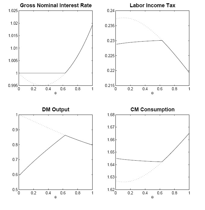
The solid line in Figure 1 shows the steady-state Ramsey policy and key allocation variables as functions of $\theta$. At $\theta = 1$, the optimal nominal interest rate is about 2 percent at an annual rate; the associated optimal inflation rate is thus -1.6 percent, higher than the Friedman rate of deflation, which would be -3.4 percent in our model.

As $\theta$ falls below unity, the optimal nominal interest rate falls. This is due to the holdup problem associated with holding money when $\theta< 1$ discussed by LW. Specifically, when $\theta< 1$, the buyer does not get the full benefit from the match and this reduces his incentive to hold money, causing the equilibrium $q$ to fall. Realizing this, the Ramsey planner reduces the inflation tax, balancing his desire to tax the buyer's surplus with the desire to reduce the effects of the holdup problem. Because seignorage revenue (not shown) falls along with the nominal interest rate, the government's revenue shortfall must be made up with the labor tax, causing the labor tax rate to rise, as the top right panel of Figure 1 shows. The associated responses of the allocation variables $q$ and $X$ are easy to understand as well. As the labor income tax rate rises with the fall in $\theta$, hours worked and hence consumption in the CM decline.

If $\theta$ falls far enough the ZLB constraint binds, making the Friedman Rule the optimal policy. For our calibration, the ZLB constraint binds if $\theta\in(0, 0.62)$, as can be seen by the fact that the net nominal interest rate is zero over that interval. The kink when the ZLB constraint binds leads to kinks in the labor tax rate and allocations as well.

The dotted line in Figure 1 shows the allocations and implied $R$ and $\tau^{h}$ that emerge from the Ramsey problem with the ZLB constraint (42) dropped. The results for $\theta\in(0.62, 1)$ are of course identical because in that region the ZLB constraint did not bind anyway. With the ZLB constraint dropped and $\theta\in(0, 0.62)$, we see that the Ramsey planner would like to implement, if it were consistent with monetary equilibrium, a negative net nominal interest rate, apparently to boost $q$. Of course, deflation faster than the Friedman Rule is inconsistent with a monetary steady-state equilibrium. Hence, the Friedman Rule becomes the constrained optimal policy.

4.2.3  Ramsey Dynamics

We now turn to the dynamics of the Ramsey policy, which reveals our second central result: optimal inflation is very stable. To investigate the dynamic behavior of our model, we solve for the dynamic Ramsey equilibrium and simulate the model. We conduct 1000 simulations of 500 periods each and discard the first 100 periods. As in Khan, King, and Wolman (2003) and others, we assume that the initial state of the economy is the asymptotic Ramsey steady-state. For each simulation, we then compute first and second moments and report the averages of these moments over the 1000 simulations.

Before turning to simulations, we make a few observations by inspecting the first-order conditions of the Ramsey problem. First, government spending affects only CM hours because none of the first-order conditions for $q_{t}$, $X_{t}$, and $\iota_{t}$ (the multiplier on the ZLB constraint) involve $G_{t}$. Once $X_{t}$ is determined, $H_{t}$ adjusts according to the shocks to $G_{t}$. This result follows from the quasi-linearity of preferences in the CM. Because households essentially have risk-neutral preferences over hours, fluctuations in $G_{t}$ are fully reflected in $H_{t}$.¹³ Simply put, the dichotomy result is that CM and DM allocations have nothing to do with each other unless production in each market depends on a common capital stock (as we introduce in Section 5). Second, and related, the dynamics of $q_{t}$ and $X_{t}$ follow the dynamics of the technology shock as the latter is the only driving force for the former. Third, for the particular utility function we choose in the CM - in fact for any CRRA utility function -- the labor income tax rate is constant over time.¹⁴ This can be viewed as the extreme case of the usual consumption-smoothing motive as spelled out in, say, Barro (1979).

Table 1 presents simulation-based moments for the key allocation and policy variables for $\theta = 1$ (which, again, is equivalent to price-taking) and for $\theta< 1$. Let us first discuss the results for $\theta = 1$. The first three rows show the dynamics of realized inflation, the labor income tax rate, and the net nominal interest rate under the Ramsey policy. We hone in first on the result that the optimal inflation rate is quite smooth over time, with a standard deviation of about only about 24 basis points (at an annual rate) around a mean deflation rate of 2 percent. The very stable inflation rate is in sharp contrast to the extremely volatile optimal inflation rate first found by CCK in a flexible-price Ramsey model and recently verified in, among others, the flexible-price versions of Schmitt-Grohe and Uribe (2004a, 2004b), Siu (2004), and Chugh (2006a, 2006b).¹⁵

In these baseline Ramsey monetary models, inflation does not distort the relative prices of goods. It is easiest to see this in a cash-credit economy: the nominal price of both cash and credit goods is $P$, and the relative price depends only on the nominal interest rate, reflecting the opportunity cost of the money used to purchase the cash good. In other words, given a nominal interest rate, dynamic fluctuations in the price level do not alter the relative price between cash and credit goods and therefore do not affect equilibrium allocations. In these baseline models, then, the driving force behind price-level dynamics is just the (desirable) ability of price-level fluctuations to tailor the real returns on nominal government debt, thus avoiding the need to change other distortionary taxes in the face of shocks to the government budget. Quantitatively, assuming business-cycle magnitude shocks, realized inflation turns out to be very volatile.¹⁶

With money essential, this result is overturned because inflation affects the relative price of DM and CM goods. To see this, note that the nominal price of a DM good in period $t$ can be expressed as $M_{t}/q_{t}$, which is simply per-unit expenditure in the DM. This means the relative price of DM goods in terms of CM goods is simply real money balances divided by DM consumption. Both of these objects are functions of inflation in equilibrium and therefore the relative price is in principle a function of inflation in equilibrium. In equilibrium, inflation thus affects the household's margin between DM and CM goods in a way that simply cannot occur in a cash-credit environment. Usual tax-smoothing reasons then suggest that it is optimal to have smooth (low-volatility) inflation because otherwise this margin would be disrupted. In Table 1 we also report the dynamic properties of this relative price, and they are quite similar to -- indeed, even smoother than -- the dynamic properties of inflation. This demonstrates that even though the Ramsey planner has available the option of moving this relative price around over time, it is optimal to not do so.

Other Ramsey models make the prediction that inflation stability is optimal, most notably Schmitt-Grohe and Uribe (2004b), Siu (2004) and Chugh (2006b). The basic mechanism behind their inflation stability results is also a relative-price distortion caused by inflation; however, these models all rely on nominal rigidities to generate the relative-price effect. We emphasize that in our model, prices are fully flexible and yet inflation causes relative price distortions. The real frictions underlying monetary exchange are behind our result.

Another perhaps noteworthy feature of inflation dynamics is that it displays high persistence. In the benchmark CCK model, which assumed fixed capital, inflation persistence is virtually zero no matter how persistent are the driving shocks. Chugh (2006a) shows that allowing for capital accumulation or habit formation generates optimal inflation persistence, but clearly here we have that result with neither of these features. If one inspects the equilibrium Euler equation for bonds, which is what we use to solve for the dynamics of inflation, it is not surprising that the dynamics of inflation would closely track the dynamics of $q_{t}$ and $X_{t}$, which in turn closely track the dynamics of the technology shock.

Finally, consider the results for $\theta< 1$, reported in the second panel of Table 1. The means of the variables of interest are of course in line with the steady state results. Compared to the price-taking case ($\theta = 1$), the average labor income tax rate is higher and average consumption (both CM and DM) and GDP are lower. The Friedman rule is optimal with an average deflation equal to the rate of time preference. In our simulations, which are driven by business-cycle-magnitude shocks, we find that the optimal nominal interest rate is once again constant over time.¹⁷ Thus, even though the ZLB constraint can be an occasionally-binding constraint in principle, for our calibration it either always binds ($\theta< 1$) or never binds ($\theta = 1$). We also find that $q_{t}$ is less volatile if $\theta< 1$, which in turn causes GDP to be less volatile and the correlations of other variables with GDP to be lower than what we find when $\theta = 1$. In short, we find that except for the expected changes in the means, the dynamic behavior of the Ramsey problem with $\theta< 1$ is qualitatively identical to the case with $\theta = 1$.

5  Model with Capital

Ramsey models of optimal fiscal and monetary policy have only recently begun considering how the presence of capital accumulation affects optimal policy.¹⁸ Here, we add capital to our baseline model following AWW: we assume that capital is accumulated in the CM and used in production in both the CM and the DM. As AWW show, with capital productive in both markets, the LW and Aruoba and Wright (2003) ``dichotomy" result, in which CM and DM allocations have nothing to do with each other, disappears. We proceed by briefly describing how the model is modified to accommodate capital and then present results.

5.1  Production

The critical change from the basic model is that capital is introduced as a factor of production in both the DM and CM. In the CM, this is done in the obvious way: production takes place according to a constant returns technology subject to TFP shocks, $Z_{t} F(K_{t},H_{t})$. Profit-maximization by firms in the CM leads to standard factor-price conditions, $w_{t} = Z_{t} F_{H} (K_{t},H_{t})$ and $r_{t} = Z_{t} F_{K}(K_{t},H_{t})$.

In the period-$t$ DM, sellers use the capital they have, which is $K_{t+1}$ according to our timing convention.¹⁹ As explained in AWW, this amounts to modifying the cost function to include capital as $c(q_{t}, K_{t+1},Z_{t})$, with $c_{k}<0$, $c_{qk}<0$ and $c_{kk}>0$.

5.2  Households

The household CM budget constraint modifies in the obvious way,

$$P_{t} x_{t} + P_{t} \left[ k_{t+1} - (1-\tau^{k} _{t})(r_{t} - \delta)k_{t}\right] + m_{t} + b_{t} = P_{t} w_{t} (1-\tau ^{h}_{t}) h_{t} + m_{t-1} + R_{t-1} b_{t-1},$$ (52)

where $k_{t}$ is the household's capital holdings at the start of period $t$, $r_{t}$ is the rental rate on capital, $\delta$ is its deprecation rate, and $\tau^{k}_{t}$ is the tax rate on capital income.²⁰ The value functions in the CM and the DM now of course include the household's capital holdings as a state variable. The household's CM problem is

$$W_{t}\left( m_{t-1}, b_{t-1}, k_{t}, S_{t}\right) = \max_{x_{t},h_{t},m_{t},b_{t},k_{t+1}} \left\{ U(x_{t}) - Ah_{t} + V_{t}(m_{t},b_{t},k_{t+1},S_{t}) \right\}$$ (53)

subject to (52).

The first order conditions of this problem are exactly as they were in the basic model, with a new condition for capital accumulation given by

$$\frac{A}{P_{t} w_{t} (1-\tau_{t}^{h})} = V_{k,t} (m_{t} ,b_{t},k_{t+1},S_{t}).$$ (54)

The results regarding the degenerate distribution of bonds and money readily extend to capital. $W_{t}(.)$ is still linear in all its arguments, with $W_{k,t}$ given by

$$W_{k,t}(m_{t-1},b_{t-1},k_{t},S_{t})=\frac{A\left[ 1+\left( r_{t}-\delta\right) \left( 1-\tau_{t}^{k} \right) \right] }{w_{t}\left( 1-\tau_{t}^{h} \right) }.$$ (55)

In the DM, we again consider two pricing schemes: bargaining and price-taking. Unlike the basic model, price-taking cannot be obtained by a simple parameter restriction of the bargaining model and as such we briefly discuss it below. The DM problem for the household is still given by (9) after obvious changes in arguments and using $(q^{b}_{t},d^{b}_{t})$ and $(q^{s}_{t},d^{s}_{t})$ to represent the terms of trade from the viewpoint of the buyers and the sellers, respectively. This simplifies to

$$V_{t}(m_{t},b_{t},k_{t+1},S_{t}) = \sigma\left\{ u\left( q^{b}_{t} \right) -c \left( q^{s}_{t}, k_{t+1},Z_{t} \right) - \beta\chi_{t} d^{b}_{t} + \beta\chi_{t} d^{s}_{t} \right\} + \beta E_{t}W_{t+1}\left( m_{t},b_{t},k_{t+1},S_{t+1}\right) .$$ (56)

using the linearity of $W_{t+1}(.)$. All we have to do to characterize the solution to the household's problem is to compute the partial derivatives of $V_{t}(.)$, which we do for both pricing schemes below. As in AWW, capital is only a productive input in this market and cannot be used as a medium of exchange. Those familiar with the AWW model may choose to skip the following exposition and proceed directly to the Ramsey problem in Section 6.

5.2.1  Household DM Problem - Bargaining

The bargaining problem is still given by (15) with the obvious modifications regarding capital. The solution to the problem gives $d(m_{t},k_{t+1},S_{t})=m_{t}$, $q=d(m_{t},k_{t+1},S_{t})$ where $q$ solves $\beta\chi_{t} m_{t} = g(q,k_{t+1},Z_{t})$, $m$ refers to the buyer's money holdings and $k$ refers to the seller's capital stock. The function $g(q_{t}, k_{t+1}, Z_{t})$ is a straightforward modification of the one in the basic model.

The only new partial derivative we need is $V_{t,k_{t+1}}$ which is given by

$$V_{k,t}\left( m_{t},b_{t},k_{t+1},S_{t}\right) =-\sigma\left[ c_{q}\left( q_{t},k_{t+1},Z_{t}\right) \frac{\partial q}{\partial k}+c_{k}\left( q_{t},k_{t+1},Z_{t}\right) \right] +\beta A E_{t}\left[ \frac{1+\left( r_{t+1}-\delta\right) \left( 1-\tau_{t+1}^{k} \right) }{w_{t+1}\left( 1-\tau_{t+1}^{h} \right) }\right]$$ (57)

Noting $\partial q/\partial k = - g_{k} / g_{q}$, defining

$$\gamma(q_{t}, K_{t+1},Z_{t}) \equiv\frac{c_{q}(q_{t}, K_{t+1},Z_{t}) g_{k}(q_{t}, K_{t+1},Z_{t}) - c_{k}(q_{t}, K_{t+1},Z_{t}) g_{q}(q_{t}, K_{t+1},Z_{t}) }{g_{q}(q_{t}, K_{t+1}Z_{t})},$$ (58)

and combining the optimality conditions (4) and (54) with the envelope condition (57), we get the household's Euler equation for capital accumulation,

$$U^{\prime}(X_{t}) = \beta E_{t} \left\{ U^{\prime }(X_{t+1}) \left[ 1 + (1-\tau^{k}_{t+1})(r_{t+1} - \delta)\right] \right\} + \sigma\gamma(q_{t}, K_{t+1},Z_{t}),$$ (59)

which shows that investment takes into account the fact that capital affects productivity in the DM as well as in the CM. The additional term related to the DM represents the seller's payoff from carrying $k_{t+1}$ units of capital into the DM and producing $q_{t}$ units, which occurs with probability $\sigma$. As such, we can think of it as the return of capital in the DM. Therefore when making an investment decision in the CM of period $t$, the households take the return of extra capital in the CM of period $t+1$, which is the usual term on the right hand side as well as the return in the DM. It is also straightforward to show that the analog of the Fisher-like condition (33) from our baseline model is

$$R_{t} = \sigma\frac{u^{\prime}(q_{t})}{g_{q}(q_{t}, K_{t+1}, Z_{t})} + 1 - \sigma,$$ (60)

which we need in order to write the ZLB constraint on the Ramsey problem.

5.2.2  Household DM Problem - Price-Taking

An alternative to bargaining is price taking, in which buyers and sellers each take the price of a unit of good in the DM, $\tilde{p}$, as given and solve their respective demand and supply problems. The buyer's problem is

$$V^{b}\left( m_{t},b_{t},k_{t+1},S_{t}\right) =\max\limits_{q}\left\{ u\left( q\right) +\beta E_{t}W_{t+1}\left( m_{t}-\tilde{p}q,b_{t} ,k_{t+1},S_{t+1}\right) \right\}$$ (61)

subject to $\tilde{p}q \leq m_{t}$. In equilibrium this constraint binds, and we have $q_{t} = M_{t}/\tilde{p}$. The seller's problem is

$$V^{s}\left( m_{t},b_{t},k_{t+1},S_{t}\right) =\max\limits_{q}\left\{ -c\left( q,k_{t+1},Z_{t}\right) +\beta E_{t}W_{t+1}\left( m_{t}+\tilde {p}q,b_{t},k_{t+1},S_{t+1}\right) \right\} ,$$ (62)

with the first order condition $c_{q}(q_{t},k_{t+1},Z_{t})=\beta\tilde{p} \chi_{t}$. Using these two expressions, the two envelope conditions we need to solve the problem of the household are given by

$$V_{m,t}\left( m_{t},b_{t},k_{t+1},S_{t}\right) =\left( 1-\sigma\right) \beta\chi_{t}+\sigma\beta\chi_{t}\frac{u^{\prime}\left( q_{t}\right) } {c_{q}\left( q_{t},k_{t+1},Z_{t}\right) }$$ (63)

$$V_{k,t}(m_{t},b_{t},k_{t+1},S_{t})=\beta A E_{t}\left[ \frac{1+\left( r_{t+1}-\delta\right) \left( 1-\tau_{t+1}^{k} \right) }{w_{t+1}\left( 1-\tau_{t+1}^{h} \right) }\right] - \sigma c_{k}(q_{t},k_{t+1},Z_{t}).$$ (64)

The analog of the Fisher-like condition (33) from our baseline model is

$$R_{t} = \sigma\frac{u^{\prime}(q_{t})}{c_{q}(q_{t}, K_{t+1}, Z_{t})} + 1 - \sigma.$$ (65)

5.3  Government

The government now collects revenue from capital income and labor income taxation, along with money creation and debt issuance. Its CM flow budget constraint is thus

$$M_{t} + B_{t} + P_{t} w_{t} \tau^{h}_{t} H_{t} + P_{t} \tau^{k}_{t} (r_{t} - \delta)K_{t} = P_{t} G_{t} + M_{t-1} + R_{t-1}B_{t-1}.$$ (66)

5.4  Equilibrium

Combining the relevant conditions derived in this section with the ones that were unchanged from the basic model, we now list the equilibrium conditions we use in writing the Ramsey problem.

5.4.1  Bargaining

Given policy variables $\{\tau^{h}_{t},\tau^{k}_{t}, R_{t}\}_{t=0}^{\infty}$, the technology realization $\{Z_{t}\}_{t=0}^{\infty}$, the government spending realization $\{G_{t}\}_{t=0}^{\infty}$, and initial condition $(M_{0} ,B_{0},K_{0})$, equilibrium is a set of processes
$\{q_{t}, B_{t}, M_{t}, K_{t}, X_{t}, H_{t}, P_{t}\}_{t=0}^{\infty}$ satisfying

$$U^{\prime}(X_{t}) = \frac{A}{(1-\tau_{t}^{h})Z_{t} F_{H}(K_{t},H_{t})},$$ (67)

$$\beta M_{t} E_{t}\left[ \frac{U^{\prime}(X_{t+1} )}{P_{t+1}}\right] = g(q_{t},K_{t+1},Z_{t}),$$ (68)

$$U^{\prime}(X_{t}) = \beta E_{t} \left\{ U^{\prime }(X_{t+1})\left[ 1 + (1-\tau^{k}_{t+1})(Z_{t+1} F_{K}(K_{t+1},H_{t+1}) - \delta)\right] \right\} + \sigma\gamma(q_{t}, K_{t+1},Z_{t}),$$ (69)

$$R_{t} = \sigma\frac{u^{\prime}(q_{t})}{g_{q}(q_{t}, K_{t+1}, Z_{t})} + 1 - \sigma,$$ (70)

$$\frac{U^{\prime}(X_{t})}{P_{t}} = \beta R_{t} E_{t} \left[ \frac{U^{\prime}(X_{t+1})}{P_{t+1}}\right]$$ (71)

$$X_{t} + G_{t} + K_{t+1} = Z_{t} F(K_{t},H_{t}) + (1 - \delta) K_{t},$$ (72)

$$M_{t} + B_{t} + P_{t} Z_{t} F_{H}(K_{t},H_{t}) \tau ^{h}_{t} H_{t} + P_{t} \tau^{k}_{t} [Z_{t} F_{K}(K_{t},H_{t}) - \delta]K_{t} = P_{t} G_{t} + M_{t-1} + R_{t-1}B_{t-1}$$ (73)

In the bargaining version, real money balances can be expressed as

$$\frac{M_{t}}{P_{t}} = \frac{g(q_{t},K_{t+1},Z_{t}) }{U^{\prime}(x_{t})} \left[ \sigma\frac{u^{\prime}(q_{t})}{g_{q} (q_{t},K_{t+1},Z_{t})} + 1 - \sigma\right] ,$$ (74)

and the ZLB constraint is

$$\sigma\left( \frac{u^{\prime}(q_{t})}{g_{q}(q_{t} ,K_{t+1},Z_{t})} - 1 \right) \geq0.$$ (75)

5.4.2  Price-Taking

Given policy variables $\{\tau^{h}_{t},\tau^{k}_{t}, R_{t}\}_{t=0}^{\infty}$, the technology realization $\{Z_{t}\}_{t=0}^{\infty}$, the government spending realization $\{G_{t}\}_{t=0}^{\infty}$, and initial condition $(M_{0} ,B_{0},K_{0})$, equilibrium is a set of processes
$\{q_{t}, B_{t}, M_{t}, K_{t}, X_{t}, H_{t}, P_{t}\}_{t=0}^{\infty}$ satisfying (67), (71), (72), and (73) along with

$$\beta M_{t} E_{t}\left[ \frac{U^{\prime}(X_{t+1} )}{P_{t+1}}\right] = q_{t} c_{q}(q_{t},K_{t+1},Z_{t}),$$ (76)

$$U^{\prime}(X_{t}) = \beta E_{t} \left\{ U^{\prime }(X_{t+1})\left[ 1 + (1-\tau^{k}_{t+1})(Z_{t+1} F_{K}(K_{t+1},H_{t+1}) - \delta)\right] \right\} - \sigma c_{k}(q_{t}, K_{t+1},Z_{t}),$$ (77)

$$R_{t} = \sigma\frac{u^{\prime}(q_{t})}{c_{q}(q_{t}, K_{t+1}, Z_{t})} + 1 - \sigma.$$ (78)

In the price-taking version, real money balances can be expressed as

$$\frac{M_{t}}{P_{t}} = \frac{q_{t} c_{q}(q_{t} ,K_{t+1},Z_{t}) }{U^{\prime}(X_{t})} \left[ \sigma\frac{u^{\prime}(q_{t} )}{c_{q}(q_{t},K_{t+1},Z_{t})} + 1 - \sigma\right] ,$$ (79)

and the ZLB constraint is

$$\sigma\left( \frac{u^{\prime}(q_{t})}{c_{q} (q_{t},K_{t+1},Z_{t})} - 1 \right) \geq0.$$ (80)

6  Ramsey Problem in Model with Capital

As we show in Appendix C.1, we can state the analog of Proposition 1 for the model with capital:

Proposition 3   The allocations in a monetary equilibrium in the model with capital satisfy the resource constraint (72), the ZLB constraint (75) for the bargaining model and (80) for the price-taking model, and the present-value implementability constraint (PVIC),

$${\small E_{0} \sum_{t=0}^{\infty} \beta^{t} \left[ U^{\prime}(X_{t}) X_{t} - A H_{t} + \sigma g(q_{t}, K_{t+1},Z_{t}) \left( \frac{u^{\prime}(q_{t})}{g_{q}(q_{t}, K_{t+1},Z_{t})} - 1\right) + \sigma\gamma(q_{t}, K_{t+1},Z_{t}) K_{t+1} \right] = U^{\prime}(X_{0}) A_{0}.}$$ (81)

for the bargaining model and

$${\small E_{0} \sum_{t=0}^{\infty} \beta^{t} \left[ U^{\prime}(X_{t}) X_{t} - A H_{t} + \sigma q_{t} c_{q}(q_{t}, K_{t+1},Z_{t}) \left( \frac{u^{\prime}(q_{t})}{c_{q}(q_{t}, K_{t+1},Z_{t})} - 1\right) - \sigma c_{k}(q_{t}, K_{t+1},Z_{t}) K_{t+1} \right] = U^{\prime}(X_{0}) A_{0}.}$$ (82)

for the price-taking model where the constant $A_{0}$ depends on $M_{0}, B_{0}$, and $K_{0}$,

$$A_{0} = \frac{M_{-1} + R_{-1}B_{-1}}{P_{0}} + \left[ 1 + (1-\tau^{k} _{0})(Z_{0} F_{K}(K_{0},H_{0}) - \delta)\right] K_{0}.$$ (83)

With the introduction of capital, the term in the PVIC that is related to the DM is similar to the one we derived in the basic model, augmented by a new term $\sigma\gamma(.)K_{t+1}$ for the bargaining model and $-\sigma c_{k}(.)K_{t+1}$ for the price-taking model. As we argued above, the expressions multiplying $K_{t+1}$ describe the DM return to holding capital in each version of the model. In our basic model, the surplus in a meeting between a buyer and seller was created due to only the actions of the buyer, who had to choose money-holdings prior to the meeting. Here, with capital, the seller also must make a decision prior to the meeting in the form of investing in capital in the previous CM. Because a household can be a buyer or a seller with symmetric probabilities $\sigma$, the two terms in the PVIC related to the DM represent the marginal surplus times the decision of the household.

The Ramsey problem is to choose $\{X_{t}, H_{t}, K_{t+1}, q_{t}\}$ to maximize

$$E_{0} \sum_{t=0}^{\infty} \beta^{t} \left\{ U(X_{t}) - A H_{t} + \sigma\left[ u(q_{t}) - c(q_{t}, K_{t+1},Z_{t})\right] \right\}$$ (84)

subject to the resource constraint (72), the PVIC ((81) for the bargaining model or (82) for the price-taking model), and the ZLB constraint ((75) for the bargaining model or (80) for the price-taking model), taking as given $\{G_{t}, Z_{t}\}$. In Appendix C.2, we list the conditions that characterize the solution to this problem, along with the conditions that let us construct the policies and prices that support the Ramsey allocation.

7  Optimal Policy in Model with Capital

As was the case in the basic model, we are able to prove analytically that the optimal nominal interest rate is positive for the bargaining model with $\theta = 1$. For $\theta< 1$ and for the price taking model, we must resort to numerical methods.

7.1  Optimal Positive Nominal Interest Rate

Most of the discussion in this section will be very brief as almost all the results from the basic model carry over to the model with capital. We begin by proving that under bargaining we have an optimal deviation from the Friedman Rule if $\theta = 1$.

Proposition 4   (Optimal Deviation from the Friedman Rule in the Model with Capital under Bargaining) Under bargaining, if $\theta = 1$, the optimal policy features a strictly positive net nominal interest rate in every period $t \geq1$.

Proof. The proof follows very closely the one for the basic model. With $\theta = 1$, we have that $g(q,K,Z) = c(q,K,Z)$ and $\gamma(q,K,Z) = 0$, and the first-order condition of the Ramsey problem with respect to $q$ is given by

$$u' - c_q = -\left(\frac{\xi}{1+\xi}\right) c \left[\frac{u'' c_q - u'c_{qq}}{[c_q]^2}\right].$$ (85)

Because the multiplier $\xi > 0$ under the Ramsey allocation as we prove in the proof of Proposition 1, $u$ is strictly concave, $c_q > 0$, and $c_{qq} > 0$, the right hand side is strictly positive. This in turn implies $u' > c_q$, and

$$\sigma \frac{u'(q_t)}{g_q(q_t, K_{t+1},Z_t)} + 1 - \sigma > 1,$$ (86)

imposing $g_q(q_t,K_{t+1},Z_t) = c_q(q_t, K_{t+1},Z_t)$ because $\theta = 1$. But this implies, by the equilibrium condition (75), that $R_t > 1$. $\qedsymbol$

The intuition is as in the basic model: the essentiality of money creates rents in the DM, which the Ramsey planner would like to tax. In this version of the model, one can think of the rent in the DM consisting of two parts, one due to holding money, realized when the household is a buyer, and one due to holding capital, realized when the household is a seller. The inflation tax is the most direct way of taxing DM activity.

7.2  Numerical Results for the Bargaining Model

7.2.1  Solution Strategy and Parameterization

We follow the same solution strategy and adopt the same functional forms as before with the following additions. The DM cost function is

$$c(q_{t}, K_{t+1},Z_{t}) =\frac{1}{Z_{t}} q_{t}^{\kappa} K_{t+1}^{1-\kappa},$$ (87)

where $\kappa\geq1$, and the CM production function is standard Cobb-Douglas, $F(K,H) = K^{\alpha}H^{1-\alpha}$ with $\alpha\in(0,1)$. We use the parameter values provided in AWW.²¹ We keep the same stochastic processes for $G_{t}$ and $Z_{t}$, but we alter $\bar{G}$ and the level of steady-state debt to match the same targets as in the basic model.

7.2.2  Ramsey Steady-State

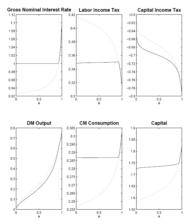
Figure 2 shows how the Ramsey steady-state varies with $\theta$ with and without the ZLB. As the upper left panel shows, the range of $\theta$ over which the ZLB constraint binds is clearly larger here than in Figure 1, but this may be due to the somewhat different parametrizations across models. It is important to note that due to Proposition 4, there will always be an interior $\bar{\theta}$ where the Friedman rule will not be optimal for all $\theta>\bar{\theta}$. Clearly, the same message as in Section 4 comes through: when $\theta$ is low enough, the ZLB constraint binds and the Friedman Rule is optimal. But for large enough $\theta$ -- in particular for the interesting case $\theta = 1$ -- the Friedman Rule is not optimal. Here, not only is the Friedman Rule not optimal, but the optimal inflation rate (not shown) is actually positive, around 7 percent, in contrast to the small deflation that was optimal in the model without capital.

The upper middle panel shows that the labor income tax rate is roughly constant at about 35 percent over $\theta\in(0,0.90)$, then falls somewhat for higher values of $\theta$. The intuition is just as before: as the inflation tax begins generating revenue, the distortionary labor income tax can be reduced.

The capital income tax rate is negative for all values of $\theta$, as the upper right panel of Figure 2 shows. Indeed, for $\theta = 1$, it is relatively easy to see that the steady-state capital tax rate in general is non-positive. Dropping the ZLB constraint (because we know it does not bind if $\theta = 1$), and using some simplifications that follow from our functional forms, the steady-state version of the Ramsey first-order condition with respect to capital is

$$-\sigma c_{k} - \rho+ \beta\rho\left[ F_{k} + 1 - \delta\right] -\sigma\xi c_{k} = 0.$$ (88)

where $\rho$ is the Ramsey multiplier on the resource constraint and we have used the fact that $\gamma(.) = 0$ and $g(.)=c(.)$. When $\theta = 1$, the steady-state household Euler equation for capital accumulation reads

$$- 1 + \beta\left[ 1 + (1-\tau^{k})(F_{K} - \delta)\right] = 0$$ (89)

again using $\gamma(.) = 0$. In a standard Ramsey model, of course, $c = c_{k} = c_{q} = 0$; comparing the two conditions then readily shows that in steady state, the optimal capital tax is zero. Here, however, using (88) and (89) and substituting in $\rho=A(1+\xi)/F_{H}$, we can solve for the capital tax rate,

$$\tau^{k} = \dfrac{\sigma c_{k} F_{H}}{A \beta(F_{K}-\delta)} < 0.$$ (90)

As long as $\sigma>0$ and $c_{k} \neq0$, which holds as long as $\kappa> 1$, the limiting capital income tax rate is negative. The crucial difference between our model and a standard Judd (1985) or Chamley (1986) argument is that the presence of the $K$ terms in the implementability constraint, arising from the trading arrangements in the DM, drive another wedge between the Ramsey and household FOCs on capital.

In terms of the economics, there are two reasons for the capital subsidy. First, there is a holdup problem for investment in this model as long as $\theta>0$, which is analogous to (and in addition to) the money holdup problem in the basic model; this holdup problem causes capital to be underaccumulated relative to the efficient capital stock. Specifically, DM sellers bear the entire cost of investment in capital but, unless $\theta= 0$, must share part of the surplus created from capital with DM buyers. Seller thus do not have the socially-correct incentive to accumulate capital. Second, the deviation from the Friedman Rule itself causes an inefficiency in the capital stock, along with other allocation variables. 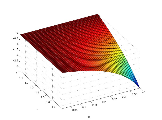The Ramsey planner subsidizes capital income in an effort to reduce the effects of both of these sources of inefficiency. In Figure 3, we plot the steady-state value of the optimal capital income tax for the $\theta = 1$ case as we vary $\kappa$ and $\sigma$.²² If $\sigma=0$, the DM shuts down and we recover the usual result that capital income is not taxed (or subsidized) because both of the channels just described are absent. If $\kappa=1$, capital is not a factor of production in the DM and the holdup problem we mention above is not present. As $\sigma$ and $\kappa$ increase, the optimal capital subsidy increases.

For our baseline parameter values, the capital income subsidies in the range 60 to 80 percent that we find in Figure 2 are large, but not out of line with capital subsidy rates found in other Ramsey studies. For example, Schmitt-Grohe and Uribe (2005, Table 2) find an optimal capital subsidy rate of 44 percent in their benchmark model featuring a host of real and nominal rigidities and report that it can be as high as 85 percent.

Optimal policies and allocations in the price-taking version of the model share the same characteristics as the bargaining version: the optimal nominal interest rate is $7.7\%$ and the capital income subsidy is $11.6\%$. The capital subsidy is lower with price-taking because price-taking avoids the capital holdup (as well as money holdup) problem inherent in Nash bargaining. If somehow the Friedman rule had been part of the Ramsey policy, then the optimal capital income tax with price-taking in fact would have been zero.

7.2.3  Ramsey Dynamics

In Table 2, we report simulation-based moments for the Ramsey allocations and policy variables for the three versions of our model with capital. While we track ex-post inflation as before, we track the ex-ante capital income tax, following the convention in much of the optimal capital taxation literature.²³ Note that, unlike in the basic model, both $Z_{t}$ and $G_{t}$ shocks affect the Ramsey solution in the models with capital. Also, while we do not analytically prove they are constant, the simulated values for the labor and capital income taxes and the nominal interest rate are essentially constant.²⁴ As such, we do not report the second moments for these variables.

Turning to the results, in all three versions of the model, we find that inflation is once again very stable, with a standard deviation of about 20 basis points at an annual rate. This is in line with the results of Chugh (2006a) and Schmitt-Grohe and Uribe (2005) in that they both also find that, so long as prices are flexible, capital accumulation does little to change the volatility of Ramsey inflation relative to a flexible-price environment without capital. That is, the volatility of Ramsey inflation has nothing to do with whether or not there is capital accumulation. Of course, in our basic model without capital, inflation was already quite stable; this result carries over unchanged. The intuition for the optimality of inflation stability is just as in the model without capital: the relative price between CM and DM consumption depends on the inflation rate, and distorting this relative price imposes welfare costs so large that the Ramsey planner largely refrains from varying inflation despite its ability to absorb shocks to the government budget.

8  Conclusion

We view our work and results as a first step in taking more seriously the new class of micro-founded models of money as a laboratory for studying policy questions. Our central findings are that the Friedman Rule is typically not the optimal policy and that inflation fluctuates very little over time. These findings are opposite those of the workhorse Chari, Christiano, and Kehoe (1991) flexible-price Ramsey model. The presence of real frictions that give rise to valued money also provide completely different justification for a central bank's pursuit of inflation stability than the typically-invoked ones of nominal rigidities.

There are of course a number of ways one might want to modify our framework. Monopoly power in goods and labor markets are thought by many to be important realistic features. It would be straightforward to introduce monopoly power in the centralized market. The results of Schmitt-Grohe and Uribe (2004a) and Chugh (2006b) suggest that inflation in such an environment would be partly a direct tax on the money rent we identify and partly an indirect tax on producers' and labor suppliers' rents. It may be interesting to know quantitatively how these direct and indirect uses of the inflation tax interact.

Once one has monopoly power in the centralized market, one could go further in adding elements monetary policy makers often think are important, such as sticky prices and sticky wages. However, given our finding of optimal inflation stability (albeit around a non-zero average inflation rate), we do not see how the results could be very different with such features.

Pushing our first step in different directions, another interesting issue to study may be the nature of and solution to the time-inconsistency problem of the Ramsey policy in this sort of environment. It is not clear how the time-consistency results of, say, Alvarez, Kehoe, and Neumeyer (2004) or Persson, Persson, and Svensson (2006), would extend to our environment. Neither is it clear how the emerging results in the new dynamic public finance literature, which places at center stage distributional concerns, might extend to a version of our environment in which money holdings were allowed to differ across individuals.

Recent developments in understanding the micro-foundations of monetary exchange are sometimes viewed as simply having provided justification for the reduced-form models of money commonly used in practice, not least of all because they superficially end up resembling the reduced-form models. Our results throw into question the conclusion that they must therefore yield the same answers to interesting questions as existing models. We think it may be worthwhile to re-examine a number of issues in monetary policy using this now-tractable framework.

A  The Ramsey Problem in Basic Model

A.1  Proof of Proposition 1

That allocations from a monetary equilibrium should satisfy the CM feasibility condition (39) and the zero-lower-bound constraint (42) is obvious.

Using the household optimality conditions (27 ), (31), and (32) along with the equilibrium conditions, we now derive the present-value implementability constraint the Ramsey planner must respect. Begin as usual with the CM household flow budget constraint,

$$P_{t} X_{t} + B_{t} + M_{t} = P_{t} w_{t} (1-\tau ^{h}_{t}) H_{t} + M_{t-1} + R_{t-1} B_{t-1}.$$ (91)

To construct the present-value implementability constraint, begin by multiplying the flow budget constraint by $\beta^{t} U^{\prime}(X_{t})/P_{t}$ and summing from $t = 0..\infty$,

$$\lefteqn{E_{0}\sum_{t=0}^{\infty} \beta^{t} U'(X_{t}) X_{t} + \sum_{t=0}^{\infty} \beta^{t} U'(X_{t}) \frac{B_{t}}{P_{t}} + \sum_{t=0}^{\infty} \beta^{t} U'(X_{t}) \frac{M_{t}}{P_{t}} = }$$ (92)

$$\sum_{t=0}^{\infty} \beta^{t} U^{\prime}(X_{t}) (1-\tau^{h}_{t})w_{t} H_{t} + \sum_{t=0}^{\infty} \beta^{t} U^{\prime}(X_{t}) \frac{M_{t-1}}{P_{t}} + \sum_{t=0}^{\infty} \beta^{t} U^{\prime}(X_{t}) \frac{R_{t-1}B_{t-1}}{P_{t}} .$$

We point out that, as usual in a dynamic Ramsey problem assuming commitment to the time-zero policy, any $E_{t}$ terms that appear in intermediate expressions are eliminated by the law of iterated expectations because the entire implementability constraint is conditioned on the time-zero information set, hence the $E_{0}$. For ease of exposition, we therefore proceed dropping $E_{t}$ operators that would appear in intermediate expressions as well as the $E_{0}$ operator because it is understood to be present in all subsequent expressions.

Substitute into the second term on the left-hand-side using expression (32) to get

$$\lefteqn{\sum_{t=0}^{\infty} \beta^{t} U'(X_{t}) X_{t} + \sum_{t=0}^{\infty} \beta^{t+1} U'(x_{t+1}) \frac{R_{t} B_{t}}{P_{t+1}} + \sum_{t=0}^{\infty} \beta^{t} U'(X_{t}) \frac{M_{t}}{P_{t}} = }$$ (93)

$$\sum_{t=0}^{\infty} \beta^{t} U^{\prime}(X_{t}) (1-\tau^{h}_{t})w_{t} H_{t} + \sum_{t=0}^{\infty} \beta^{t} U^{\prime}(X_{t}) \frac{M_{t-1}}{P_{t}} + \sum_{t=0}^{\infty} \beta^{t} U^{\prime}(X_{t}) \frac{R_{t-1}B_{t-1}}{P_{t}} .$$ (94)

The second summation on the left-hand-side cancels with the the last summation on the right-hand-side to leave only the initial bond position,

$$\lefteqn{\sum_{t=0}^{\infty} \beta^{t} U'(X_{t}) X_{t} + \sum_{t=0}^{\infty} \beta^{t} U'(X_{t}) \frac{M_{t}}{P_{t}} = }$$ (95)

$$\sum_{t=0}^{\infty} \beta^{t} U^{\prime}(X_{t}) (1-\tau^{h}_{t})w_{t} H_{t} + \sum_{t=0}^{\infty} \beta^{t} U^{\prime}(X_{t}) \frac{M_{t-1}}{P_{t}} + U^{\prime}(x_{0}) \frac{R_{-1}B_{-1}}{P_{0}}.$$ (96)

Next, substitute into the second term on the left-hand-side using (31) to get

$$\lefteqn{\sum_{t=0}^{\infty} \beta^{t} U'(X_{t}) X_{t} + \sum_{t=0}^{\infty} \beta^{t+1} U'(x_{t+1}) \frac{M_{t}}{P_{t+1}} \left[ \sigma\frac{u'(q_{t} )}{g'(q_{t})} + 1 - \sigma\right] = }$$ (97) (98)

$$\sum_{t=0}^{\infty} \beta^{t} U^{\prime}(X_{t}) (1-\tau^{h}_{t})w_{t} H_{t} + \sum_{t=0}^{\infty} \beta^{t} U^{\prime}(X_{t}) \frac{M_{t-1}}{P_{t}} + U^{\prime}(x_{0}) \frac{R_{-1}B_{-1}}{P_{0}}.$$
Expand the second summation on the left-hand-side to get

$$\lefteqn{\sum_{t=0}^{\infty} \beta^{t} U'(X_{t}) X_{t} + \sum_{t=0}^{\infty} \beta^{t+1} U'(x_{t+1}) \frac{M_{t}}{P_{t+1}} + \sigma\sum_{t=0}^{\infty} \beta^{t+1} U'(x_{t+1}) \frac{M_{t}}{P_{t+1}} \left[ \frac{u'(q_{t} )}{g'(q_{t})} -1 \right] }$$ (99)

$$= \sum_{t=0}^{\infty} \beta^{t} U^{\prime}(X_{t}) (1-\tau^{h}_{t})w_{t} H_{t} + \sum_{t=0}^{\infty} \beta^{t} U^{\prime}(X_{t}) \frac{M_{t-1}}{P_{t}} + U^{\prime}(x_{0}) \frac{R_{-1}B_{-1}}{P_{0}}.$$ (100)

Cancel the second summation on the left-hand-side with the second summation on the right-hand-side to leave only the initial money holdings,

$$\lefteqn{\sum_{t=0}^{\infty} \beta^{t} U'(X_{t}) X_{t} + \sigma\sum _{t=0}^{\infty} \beta^{t+1} U'(x_{t+1}) \frac{M_{t}}{P_{t+1}} \left[ \frac{u'(q_{t})}{g'(q_{t})} -1 \right] }$$ (101)

$$= \sum_{t=0}^{\infty} \beta^{t} U^{\prime}(X_{t}) (1-\tau^{h}_{t})w_{t} H_{t} + U^{\prime}(x_{0}) \left[ \frac{M_{-1} + R_{-1}B_{-1}}{P_{0}}\right] .$$ (102)

Using (27), we can substitute into the first term on the right-hand-side to get

$$\sum_{t=0}^{\infty} \beta^{t} U^{\prime}(X_{t}) X_{t} - \sum_{t=0}^{\infty} \beta^{t} A H_{t} + \sigma\sum_{t=0}^{\infty} \beta^{t+1} U^{\prime}(x_{t+1}) \frac{M_{t}}{P_{t+1}} \left[ \frac{u^{\prime}(q_{t})}{g_{q}(q_{t},Z_{t})} -1 \right] = U^{\prime}(x_{0}) \left[ \frac{M_{-1} + R_{-1}B_{-1}}{P_{0} }\right] .$$ (103)

Writing $\frac{M_{t}}{P_{t+1}} = \frac{M_{t}}{P_{t}} \frac{P_{t}}{P_{t+1}}$ , express this as

$$\sum_{t=0}^{\infty} \beta^{t} U^{\prime}(X_{t}) X_{t} - \sum_{t=0}^{\infty} \beta^{t} A H_{t} + \sigma\sum_{t=0}^{\infty} \beta^{t+1} U^{\prime}(x_{t+1}) \frac{M_{t}}{P_{t+1}} \left[ \frac{u^{\prime}(q_{t})}{g_{q}(q_{t},Z_{t})} -1 \right] = U^{\prime}(x_{0}) \left[ \frac{M_{-1} + R_{-1}B_{-1}}{P_{0} }\right] .$$ (104)

Use (41) to substitute for $M_{t}/P_{t}$,

$$\sum_{t=0}^{\infty} \beta^{t} U^{\prime}(X_{t}) X_{t} - \sum_{t=0}^{\infty} \beta^{t} A H_{t} + \sigma\sum_{t=0}^{\infty} \beta^{t+1} \frac{U^{\prime }(x_{t+1})}{P_{t+1}} \frac{P_{t}}{U^{\prime}(X_{t})} g(q_{t},Z_{t}) \left[ \sigma\frac{u^{\prime}(q_{t})}{g_{q}(q_{t},Z_{t})} + 1 - \sigma\right] \left[ \frac{u^{\prime}(q_{t})}{g_{q}(q_{t},Z_{t})} -1 \right]$$ (105)

$$= U^{\prime}(x_{0}) \left[ \frac{M_{-1} + R_{-1}B_{-1}}{P_{0}}\right] .$$

Finally, from (31), we can make the substitution $\beta E_{t} \left[ \frac{U^{\prime}(x_{t+1})}{P_{t+1}}\right] = \frac{U^{\prime}(X_{t} )}{P_{t}} \left[ \sigma\frac{u^{\prime}(q_{t})}{g_{q}(q_{t},Z_{t})} + 1 - \sigma\right] ^{-1}$ in the third summation on the left-hand-side. Cancelling terms and reintroducing the $E_{0}$ operator leaves us with

$$E_{0} \sum_{t=0}^{\infty} \beta^{t} \left[ U^{\prime}(X_{t}) X_{t} - A H_{t} + \sigma g(q_{t},Z_{t}) \left( \frac{u^{\prime}(q_{t})}{g_{q}(q_{t},Z_{t})} - 1\right) \right] = U^{\prime}(x_{0}) \left[ \frac{M_{-1} + R_{-1} B_{-1} }{P_{0}} \right] ,$$ (106)

which is the present-value implementability (PVIC) constraint for the Ramsey problem in the LW model. Any allocation that satisfies this restriction, the resource constraint, and the ZLB constraint can be supported as a monetary equilibrium; furthermore, the allocations from any monetary equilibrium can be described by these three conditions.

A.2  The Solution to the Ramsey Problem

The Kuhn-Tucker conditions for the problem in Section 3 are

$$\left[ u^{\prime}(q_{t}) - c_{q}(q_{t},Z_{t})\right]$$

$$+ \xi\left[ g_{q}(q_{t},Z_{t})\left( \dfrac{u^{\prime}(q_{t})} {g_{q}(q_{t},Z_{t})} - 1\right) + g(q_{t},Z_{t})\left( \dfrac{u^{\prime \prime}(q_{t})g_{q}(q_{t},Z_{t}) - u^{\prime}(q_{t}) g_{qq}(q_{t},Z_{t} )}{[g_{q}(q_{t},Z_{t})]^{2}} \right) \right]$$ (107)

$$+\iota_{t} \left[ \dfrac{u^{\prime\prime}(q_{t})g_{q}(q_{t},Z_{t} )-u^{\prime}(q_{t})g_{q}q(q_{t},Z_{t})}{g_{q}(q_{t},Z_{t})^{2}} \right] = 0,$$

$$U^{\prime}(X_{t})-\dfrac{A}{Z_{t}}+\xi\left[ U^{\prime\prime}(X_{t} )X_{t}+U^{\prime}(X_{t})-\dfrac{A}{Z_{t}} \right] = 0,$$ (108)

$$X_{t} + G_{t} = Z_{t} H_{t}$$ (109)

$$E_{0} \sum_{t=0}^{\infty} \beta^{t} \left[ U^{\prime}(X_{t}) X_{t} - A H_{t} + \sigma g(q_{t},Z_{t}) \left( \dfrac{u^{\prime}(q_{t})}{g_{q} (q_{t},Z_{t})} - 1\right) \right] = U^{\prime}(x_{0}) \left[ \dfrac{M_{-1} + R_{-1} B_{-1}}{P_{0}} \right]$$ (110)

$$\iota_{t} \left[ \dfrac{u^{\prime}(q_{t})}{g_{q}(q_{t},Z_{t})} - 1 \right] = 0, \iota_{t} \geq0$$ (111)

We can represent the right-hand side of the PVIC in terms of allocations as

$$U^{\prime}(X) \left[ \dfrac{g(q,1)}{\beta U^{\prime}(X)} + \dfrac {\mathcal{B}}{\beta} \right]$$ (112)

where $\mathcal{B}$ is the steady state real bond balances and variables without subscripts are steady state values.

With these FOCs in hand, we proceed as follows. Imposing steady state on these conditions, we solve for the steady state values of allocations and the multiplier $\xi$. Next, given $\xi$ and $\{Z_{t},G_{t}\}$, the conditions above characterize $\{q_{t},X_{t},\iota_{t}\}$ and (39) defines $\{H_{t}\}$. Finally, we back out policies $\{\tau_{t}^{h},R_{t}\}$ from (35) and (38) statically, and inflation can be obtained from solving (37) dynamically.

B  Alternative Instruments in the DM in Basic Model

Here, we prove a claim we make in Section 4.1. To demonstrate that the deviation from the Friedman Rule in our basic model is not proxying for a sales tax in the DM, we modify our basic model. We introduce a sales tax in the DM and show that the resulting Ramsey problem does not have a solution in which the Friedman Rule holds. Our result here is only for the case $\theta = 1$ (which is equivalent to price-taking in the DM), just as is our Proposition 2. It is somewhat easier to work with the price-taking version to establish this result, which is why we use this version here.

We introduce a DM sales tax in the following way: with price-taking in the DM, buyers, taking $\tilde{P}_{t}$ as given, turn over $\tilde{P}_{t} q_{t}$ units of money in each transaction. The sellers must remit $\tau^{d}_{t} \tilde {P}_{t} q_{t}$ to the government in the next CM, which, given our timing assumptions, occurs in period $t+1$.²⁵Equivalently, we can suppose that the government receives the revenue in the DM but waits until the next CM to spend it. Because the assets markets are not open in the DM, the government cannot invest this extra revenue in an interest-bearing asset.

The government's flow budget constraint in nominal terms is thus

$$M_{t} + B_{t} + P_{t} w_{t} \tau^{h}_{t} H_{t} + \sigma\tau^{d}_{t-1} \tilde{P}_{t-1} q_{t-1} = P_{t} G_{t} + M_{t-1} + R_{t-1} B_{t-1},$$ (113)

in which the $\sigma$ appears because it is only DM sellers in period $t-1$ (of which there is a measure $\sigma$) that turn over sales taxes to the government. Because in equilibrium, $M_{t-1} = \tilde{P}_{t-1} q_{t-1}$ (that is, any DM meeting in which a transaction occurs leads to the buyer turning over all his cash to the seller), we may write the period-$t$ government budget constraint as

$$M_{t} + B_{t} + P_{t} w_{t} \tau^{h}_{t} H_{t} = P_{t} G_{t} + (1-\sigma \tau^{d}_{t-1}) M_{t-1} + R_{t-1} B_{t-1}.$$ (114)

If we sum the CM budget constraints of all households (a measure $\sigma$ of whom were buyers in period $t-1$ and thus enter period $t$ with no money; a measure $\sigma$ of whom were sellers and thus enter period $t$ with $M_{t-1}+(1-\tau^{d}_{t-1})M_{t-1}$; and a measure $1-2\sigma$ of whom did not trade and thus have $M_{t-1}$), we have in equilibrium

$$P_{t} X_{t} + M_{t} + B_{t} = P_{t} w_{t} (1-\tau^{h}_{t}) H_{t} + (1-\sigma\tau^{d}_{t-1}) M_{t-1} + R_{t-1} B_{t-1}.$$ (115)

Clearly, the government budget constraint and the summation of all the households' budget constraints yields the CM resource constraint. In the Ramsey problem, then, we can use the resource constraint and the summation of all households' budget constraints, which implies the government budget constraint is satisfied.

In order to solve the Ramsey problem, first let us derive the equilibrium conditions with this new tax instrument in place. To keep the discussion short, we simply point out the differences from the conditions we derive above. The CM problem summarized in (2)-(6) is unchanged. In the DM, from the buyer's problem (derived as in, say, Rocheteau and Wright (2005)), we get

$$\tilde{P}_{t} q_{t} = m_{t}.$$ (116)

The seller's problem can be written as

$$V^{s}\left( m_{t},b_{t},S_{t}\right) =\max\limits_{q_{t}}\left\{ -c\left( q_{t},Z_{t}\right) +\beta E_{t}W_{t+1}\left( m_{t}+(1-\tau^{d}_{t})\tilde {p}q,b_{t},S_{t+1}\right) \right\} ,$$ (117)

with the first order condition $c_{q}(q_{t},k_{t+1},Z_{t})=\beta(1-\tau ^{d}_{t})\tilde{p} \chi_{t}$ , which leads to the following expression for $V_{m}$:

$$V_{m,t}\left( m_{t},b_{t},S_{t}\right) =\left( 1-\sigma\right) \beta \chi_{t}+\sigma\beta\chi_{t}\frac{(1-\tau^{d}_{t})u^{\prime}\left( q_{t}\right) }{c_{q}\left( q_{t},Z_{t}\right) }.$$ (118)

This leads to the following equilibrium condition, which replaces (37),

$$\frac{U^{\prime}(X_{t})}{P_{t}} = \beta\left[ \sigma\frac{(1-\tau^{d} _{t})u^{\prime}(q_{t})}{c_{q}(q_{t},Z_{t})} + 1 - \sigma\right] E_{t} \left[ \frac{U^{\prime}(X_{t+1})}{P_{t+1}}\right] .$$ (119)

It is also straightforward to show that the analog of the Fisher-like condition (33) from our baseline model is

$$R_{t} = \sigma\frac{(1-\tau^{d}_{t})u^{\prime}(q_{t})}{c_{q}(q_{t}, Z_{t})} + 1 - \sigma,$$ (120)

which we need in order to write the ZLB constraint on the Ramsey problem. Note that in the main text we assumed $c(q,Z)=q/Z$ which is simply a normalization because $c(.)$ is in terms of utility. Using this, we have $c_{q}(q,Z) = 1/Z$. Also note that by construction $Z>0$.

To construct the PVIC in this version of the model, we proceed exactly as in Appendix A.1, using (115). The resulting PVIC is given by

$$E_{0} \sum_{t=0}^{\infty} \beta^{t} \left[ U^{\prime}(X_{t}) X_{t} - A H_{t} + \sigma q_{t} \left[ Z_{t}(1-\tau^{d}_{t})u^{\prime}(q_{t}) - 1\right] + \sigma\tau_{t}^{d} q_{t} \right] = U^{\prime}(x_{0}) \left[ \frac{M_{-1} + R_{-1} B_{-1}}{P_{0}} \right] - \frac{\sigma\tau_{0}^{d} q_{0}}{\beta}.$$ (121)

As usual, the Ramsey problem is to maximize the consumer's lifetime utility subject to the resource constraint, the PVIC, and the ZLB constraint. In the timeless solution of the Ramsey problem, which is what we restrict attention to, the initial tax rate $\tau^{d}_{0}$ is endogenous and equal to the steady-state $\tau^{d}$ implied by the $t>0$ Ramsey first-order conditions.

The sales tax has a natural upper bound, unity, but it does not have a natural lower bound. Denote by $\tau_{L}$ the lower bound of $\tau_{t}^{d}$. We think $\tau_{L} \leq0$ is the most natural case to consider.

We proceed by stating and proving two lemmas. The first lemma shows that the Ramsey planner always chooses $\tau_{t}^{d} = \tau_{L}$ for all $t$. The second lemma shows that if $\tau_{L} \leq0$, the ZLB cannot be binding, meaning that the Friedman Rule cannot be a part of the Ramsey policy. Thus, we establish through these two lemmas that the Friedman Rule cannot be part of the Ramsey policy even in the presence of a sales tax in the DM.

Lemma 1   The solution to the Ramsey problem with a DM sales tax features $\tau_{t}^{d} = \tau_{L}$.

Proof. Associating the multiplier $\xi$ with the PVIC and the multiplier $\iota_t$ with the ZLB constraint

$$\sigma \left [Z_t(1-\tau^d_t)u'(q_t) - 1\right] \geq 0,$$ (122)

the Ramsey first-order-conditions with respect to $\tau^d_t$ is

$$\xi \sigma q_{t}\left[ - Z_t u^{\prime }\left( q_{t}\right) +1\right] -\sigma Z_t \iota _{t}u^{\prime }\left( q_{t}\right) \leq 0, = 0 \tau_t^h > \tau_L.$$ (123)

In any monetary equilibrium, we have $q_t \in (0,q^*_t]$. This means $Z_t u'(q_t) - 1 \geq 0$ because $q^*_t$ solves $Z_t u'(q_t)-1=0$ and the utility function is strictly increasing. Examining this first order condition and given that the utility function is strictly increasing and strictly concave (and realizing the multipliers $\xi$ and $\iota$ are non-negative), the left-hand-side is strictly negative. This means the Ramsey planner wants to choose the smallest possible $\tau_t^d$, $\tau^d_t = \tau_L$. $\qedsymbol$

Lemma 2   If $\tau_{L} \leq0$, the solution to the Ramsey problem with a DM sales tax cannot feature a binding ZLB constraint.

Proof. In Proposition 1, we implicitly had $\tau_L = 0$ and showed the Friedman Rule was not optimal (meaning the ZLB constraint was not binding). Now assume $\tau_L < 0$. Given that we focus on monetary equilibria (i.e., $q_t \in (0,q^*_t]$), we have $Z_t u'(q_t) - 1 \geq 0$. We know from the lemma above that $\tau_t^d = \tau_L$. If $\tau_L < 0$, then $[(1-\tau_L) Z_t u'(q_t) - 1] > 0$, which means the ZLB constraint is slack. $\qedsymbol$

This completes our argument that if we introduce a sales tax in the DM, the Ramsey problem has no solution that includes the Friedman rule as part of the optimal policy.

C  The Ramsey Problem in Model with Capital

C.1  Proof of Proposition 3

The proof is similar to the proof of Proposition 1. Here we only show how to derive the PVIC for the bargaining version of the model. The expression for the price-taking version follows the same steps.

Having derived the implementability constraint for the LW model in Appendix A.1, it is straightforward to extend it for the AWW environment. Multiplying the consumer's CM budget constraint by $\beta^{t} U^{\prime}(X_{t})/P_{t}$ and then summing over dates and states beginning at $t=0$ as above, we have

$$E_{0} ... + \sum_{t=0}^{\infty} \beta^{t} U^{\prime}(X_{t}) K_{t+1} = \sum_{t=0}^{\infty} \beta^{t} U^{\prime}(X_{t}) \left[ 1 + (1-\tau^{k} _{t})(F_{K}(K_{t},H_{t}) - \delta)\right] K_{t} + ...$$ (124)

where the ellipsis indicate that the other terms are the same as those in (92). The manipulations following (92) proceed just as before (with, of course, $K$ now included inside the function $g(.)$), so we present here only the derivation of the terms in the implementability constraint arising from the inclusion of capital.

Use the household's Euler equation for capital,

$$U^{\prime}(X_{t}) = \beta U^{\prime}(X_{t+1}) \left[ 1 + (1-\tau^{k} _{t+1})(F_{K}(K_{t+1},H_{t+1}) - \delta)\right] + \sigma\gamma(q_{t}, K_{t+1}),$$ (125)

to substitute for $U^{\prime}(X_{t})$ on the left-hand-side of the previous expression to get

$$\lefteqn{... + \sum_{t=0}^{\infty} \beta^{t+1} U'(X_{t+1}) \left[ 1 + (1-\tau^{k}_{t+1})(F_{K}(K_{t+1},H_{t+1}) - \delta)\right] K_{t+1} }$$ (126)

$$+- \sum_{t=0}^{\infty} \beta^{t} \sigma\gamma(q_{t}, K_{t+1}) K_{t+1} = \sum_{t=0}^{\infty} \beta^{t} U^{\prime}(X_{t}) \left[ 1 + (1-\tau^{k} _{t})(F_{K}(K_{t},H_{t}) - \delta)\right] K_{t} + ...$$ (127)

Canceling like summations leaves

$$... + \sum_{t=0}^{\infty} \beta^{t} \sigma\gamma(q_{t}, K_{t+1}) K_{t+1} = U^{\prime}(X_{0}) \left[ 1 + (1-\tau^{k}_{0})(F_{K}(K_{0},H_{0}) - \delta)\right] K_{0} + ...$$ (128)

Re-inserting the terms from the LW PVIC, the PVIC for the AWW model is

$$\lefteqn{E_{0} \sum_{t=0}^{\infty} \beta^{t} \left[ U^{\prime}(X_{t}) X_{t} - A H_{t} + \sigma g(q_{t},K_{t+1}) \left( \frac{u^{\prime}(q_{t})}{g_{q} (q_{t},K_{t+1})} - 1\right) + \sigma\gamma(q_{t},K_{t+1}) K_{t+1} \right] }$$

$$= U^{\prime}(x_{0}) \left[ \frac{M_{-1} + R_{-1} B_{-1}}{P_{0}} + \left[ 1 + (1-\tau^{k}_{0})(F_{K}(K_{0},H_{0}) - \delta)\right] K_{0} \right] ,$$ (129)

which is expression (81) in the text. Any allocation that satisfies this restriction, the resource constraint, and the ZLB constraint can be supported as a monetary equilibrium; furthermore, any monetary equilibrium can be described by these three conditions.

C.2  The Solution to the Ramsey Problem

Here we only describe the solution for the bargaining version of the model and the price-taking version is similar. The Kuhn-Tucker conditions for the problem in Section 6 are

$$\left[ u^{\prime}(q_{t}) - c_{q}(q_{t},K_{t+1},Z_{t})\right] + \xi\left[ g_{q}(q_{t},K_{t+1},Z_{t})\left( \dfrac{u^{\prime}(q_{t})}{g_{q} (q_{t},K_{t+1},Z_{t})} - 1\right) \right]$$

$$+ \xi\left[ g(q_{t},K_{t+1},Z_{t})\left( \dfrac{u^{\prime\prime} (q_{t})g_{q}(q_{t},K_{t+1},Z_{t}) - u^{\prime}(q_{t}) g_{qq}(q_{t} ,K_{t+1},Z_{t})}{[g_{q}(q_{t},K_{t+1},Z_{t})]^{2}} \right) + \gamma_{q} (q_{t},K_{t+1},Z_{t})K_{t+1}\right]$$ (130)

$$+\iota_{t} \left[ \dfrac{u^{\prime\prime}(q_{t})g_{q}(q_{t},K_{t+1} ,Z_{t})-u^{\prime}(q_{t})g_{qq}(q_{t},K_{t+1},Z_{t})}{g_{q}(q_{t} ,K_{t+1},Z_{t})^{2}} \right] = 0,$$

$$U^{\prime}(X_{t})-\dfrac{A(1+\xi)}{Z_{t} F_{H}(K_{t},H_{t})}+\xi\left[ U^{\prime\prime}(X_{t})X_{t}+U^{\prime}(X_{t})\right] = 0,$$ (131)

$$- \sigma c_{k}(q_{t},K_{t+1},Z_{t}) - \dfrac{A(1+\xi)}{Z_{t} F_{H} (K_{t},H_{t}} + \beta E_{t} \left\{ \dfrac{A(1+\xi)}{Z_{t+1} F_{H} (K_{t+1},H_{t+1})} \left[ Z_{t+1} F_{K}(K_{t+1},H_{t+1}) + 1 - \delta\right] \right\}$$

$$+\sigma\xi g_{k}(q_{t},K_{t+1},Z_{t}) \left( \dfrac{u^{\prime}(q_{t} )}{g_{q}(q_{t},K_{t+1},Z_{t})} - 1\right) - \sigma\xi\dfrac{g(q_{t} ,K_{t+1},Z_{t})u^{\prime}(q_{t})g_{qk}(q_{t},K_{t+1},Z_{t})}{g_{q} (q_{t},K_{t+1},Z_{t})^{2}}$$ (132)

$$+ \sigma\xi\gamma_{k}(q_{t},K_{t+1},Z_{t})K_{t+1}+ \sigma\xi\gamma (q_{t},K_{t+1},Z_{t}) - \sigma\iota_{t} \dfrac{u^{\prime}(q_{t})g_{qk} (q_{t},K_{t+1},Z_{t})}{g_{q}(q_{t},K_{t+1},Z_{t})^{2}}=0,$$

$$X_{t} + G_{t} + K_{t+1} = (1 - \delta) K_{t} + Z_{t} F(K_{t},H_{t})$$ (133)

$$E_{0} \sum_{t=0}^{\infty} \beta^{t} \left[ U^{\prime}(X_{t}) X_{t} - A H_{t} + \sigma g(q_{t},K_{t+1}) \left( \dfrac{u^{\prime}(q_{t})}{g_{q} (q_{t},K_{t+1})} - 1\right) - \sigma\gamma(q_{t},K_{t+1}) K_{t+1} \right]$$

$$= U^{\prime}(x_{0}) \left[ \dfrac{M_{-1} + R_{-1} B_{-1}}{P_{0}} + \left[ 1 + (1-\tau^{k}_{0})(F_{K}(K_{0},H_{0}) - \delta)\right] K_{0} \right] ,$$ (134)

$$\iota_{t} \sigma\left[ \dfrac{u^{\prime}(q_{t})}{g_{q}(q_{t},K_{t+1} ,Z_{t})} - 1 \right] = 0, \iota_{t} \geq0$$ (135)

We can represent the right-hand side of the PVIC in terms of allocations as

$$U^{\prime}(X) \left[ \dfrac{g(q,1}{\beta U^{\prime}(X)} + \dfrac{\mathcal{B} }{\beta} \right] + \dfrac{U(X)}{\beta} K \left[ 1 - \sigma\dfrac {\gamma(q,K,1)}{U^{\prime}(X)} \right]$$ (136)

With these FOCs in hand, we proceed as follows. Imposing steady state on these conditions, we solve for the steady state values of allocations and the multiplier $\xi$. Next, given $\xi$ and $\{Z_{t},G_{t}\}$, the conditions above characterize $\{q_{t},X_{t},K_{t},H_{t},\iota_{t}\}$. We back out policies $\{\tau_{t}^{h},R_{t}\}$ from (67) and (70) statically. Finally capital income tax and inflation can be solved dynamically from (71) and (69).

References

Alvarez, Fernando, Patrick J. Kehoe, and Pablo Andres Neumeyer, 2004, The Time Consistency of Optimal Monetary and Fiscal Policies, Econometrica, 72, 541-567.

Aruoba, S. Boragan, Jesus Fernandez-Villaverde, and Juan F. Rubio-Ramirez, 2006, Comparing Solution Methods for Dynamic Equilibrium Economies, Journal of Economic Dynamics and Control.

Aruoba, S. Boragan, Christoper J. Waller, and Randall Wright, 2006, Money and Capital, University of Maryland.

Aruoba, S. Boragan and Randall Wright, 2003, Search, Money, and Capital: A Neoclassical Dichotomy, Journal of Money, Credit, and Banking, 35, 1086-1105.

Atkinson, Anthony B. and Joseph E. Stiglitz, 1980, Lectures on Public Economics, New York: McGraw Hill.

Barro, Robert J, 1979, On the Determination of the Public Debt, Journal of Political Economy, 87, 940-971.

Chamley, Christophe, 1986, The Welfare Cost of Capital Income Taxation in a Growing Economy, Econometrica, 54, 607-622.

Chari, V.V., Lawrence Christiano, and Patrick Kehoe, 1991, Optimal Fiscal and Monetary Policy: Some Recent Results, Journal of Money, Credit, and Banking, 23, 519-539.

Chari V. V., and Patrick J. Kehoe, 1999, Optimal Fiscal and Monetary Policy, Handbook of Macroeconomics, John B. Taylor and Michael Woodford, Vol. 1C, Elsevier.

Chugh, Sanjay K, 2006a, Optimal Inflation Persistence: Ramsey Taxation with Capital and Habits, Journal of Monetary Economics.

Chugh, Sanjay K, 2006b, Optimal Fiscal and Monetary Policy with Sticky Wages and Sticky Prices, Review of Economic Dynamics.

Howitt, Peter, 2003, Comment On: Search, Money, and Capital: A Neoclassical Dichotomy, Journal of Money, Credit, and Banking, 35, 1107-1110

Judd, Kenneth L, 1985, Redistributive Taxation in a Simple Perfect Foresight Model, Journal of Public Economics, 28, 59-83.

Judd, Kenneth L, 1992, Projection Methods for Solving Aggregate Growth Models, Journal of Economic Theory, 58, 410-452

Khan, Aubhik, Robert G. King and Alexander L. Wolman, 2003, Optimal Monetary Policy, Review of Economic Studies, 70, 825-860.

Kiyotaki, Nobuhiro and Randall Wright, 1989, On Money As a Medium of Exchange, Journal of Political Economy, 97, 927-954.

Kiyotaki, Nobuhiro and Randall Wright, 1993, A Search-Theoretic Approach to Monetary Economics, American Economic Review, 83, 63-77.

Kocherlakota, Narayana R, 1998, Money is Memory, Journal of Economic Theory, 81, 232-251.

Kocherlakota, Narayana R, 2005, Optimal Monetary Policy: What We Know and What We Don't Know, Federal Reserve Bank of Minneapolis Quarterly Review, 29, 10-19.

Lagos, Ricardo and Randall Wright, 2005, A Unified Framework for Monetary Theory and Policy Analysis, Journal of Political Economy, 113, 463-484.

Lucas, Robert E. Jr. and Nancy L. Stokey, 1983, Optimal Fiscal and Monetary Policy in an Economy Without Capital, Journal of Monetary Economics, 12, 55-93.

Persson, Mats, Torsten Persson, and Lars E. O. Svensson, 2006, Time Consistency of Fiscal and Monetary Policy: A Solution, Econometrica, 74, 193-212.

Rocheteau, Guillaume and Randall Wright, 2005, Money in Search equilibrium, in Competitive Equilibrium, and in Competitive Search Equilibrium, Econometrica, 73, 175-202.

Schmitt-Grohe, Stephanie and Martin Uribe, 2004a, Optimal Fiscal and Monetary Policy Under Imperfect Competition, Journal of Macroeconomics, 26, 183-209.

Schmitt-Grohe, Stephanie and Martin Uribe, 2004b, Optimal Fiscal and Monetary Policy Under Sticky Prices, Journal of Economic Theory, 114, 198-230.

Schmitt-Grohe, Stephanie and Martin Uribe, 2005, Optimal Fiscal and Monetary Policy in a Medium-Scale Macroeconomic Model, 2005.

Siu, Henry E, 2004, Optimal Fiscal and Monetary Policy with Sticky Prices, Journal of Monetary Economics, 51, 576-607.

Figure 1 - Ramsey Steady-State in the Basic Model

Notes : Ramsey steady-state policy and allocation as a function of $\theta$ with the ZLB constraint (solid line) and without the ZLB constraint (dotted line).

Figure 2 - Ramsey Steady-State in the Model with Capital

Notes : Ramsey steady-state policy and allocation as a function of $\theta$ with the ZLB constraint (solid line) and without the ZLB constraint (dotted line).

Figure 3 - Ramsey Steady-State Capital Income Tax

Notes : Optimal steady-state capital income tax rate as functions of $\kappa$ and $\sigma$. Buyer bargaining power fixed at $\theta = 1$.

Table 1 - Simulation Results for the Basic Model: (a) Price-Taking / Bargaining ($\theta= 1$)

Variable	Mean	Std. Dev.	Auto corr.	Corr$(x,Y)$	Corr$(x,Z)$	Corr$(x,G)$
$\pi-1$	-1.987	0.240	0.805	0.722	0.999	0.005
$\tau^{h}$	0.220	0	-	-	-	-
$R -1$	1.931	0	-	-	-	-
$q$	0.798	0.036	0.806	0.723	1.000	0.005
$X$	1.664	0.020	0.806	0.723	1.000	0.005
$H$	2.065	0.028	0.874	0.554	-0.167	0.985
$GDP$	2.263	0.040	0.840	1	0.723	0.689
$P_{DM}/P$	0.795	0.000	0.806	0.722	0.999	0.005

Table 1 - Simulation Results for the Basic Model: (b) Bargaining ($\theta< 1$)

Variable	Mean	Std. Dev.	Auto corr.	Corr$(x,Y)$	Corr$(x,Z)$	Corr$(x,G)$
$\pi-1$	-3.844	0.236	0.805	0.681	0.999	0.005
$\tau^{h}$	0.277	0	-	-	-	-
$R -1$	0	0	-	-	-	-
$q$	0.573	0.017	0.806	0.683	1.000	0.005
$X$	1.287	0.015	0.806	0.683	1.000	0.005
$H$	1.688	0.028	0.874	0.600	-0.166	0.985
$GDP$	2.024	0.038	0.844	1	0.683	0.729
$P_{DM}/P$	1.173	0.000	0.806	0.682	1.000	0.005

Notes: Simulation-based moments. Inflation and nominal interest rate reported in percentage points.

Table 2 - Simulation Results for the Model with Capital: (a) Bargaining ($\theta= 1$)

Variable	Mean	Std. Dev.	Auto corr.	Corr$(x,Y)$	Corr$(x,Z)$	Corr$(x,G)$
$\pi-1$	7.141	0.203	0.714	-0.567	-0.375	-0.383
$\tau^{h}$	0.317	0	-	-	-	-
$\tau^{k}$	-0.797	0	-	-	-	-
$R -1$	9.761	0	-	-	-	-
$q$	0.754	0.011	0.928	0.812	0.915	0.093
$K$	1.827	0.038	0.979	0.530	0.594	0.132
$X$	0.302	0.005	0.940	0.572	0.841	-0.247
$H$	0.322	0.007	0.783	0.762	0.389	0.802
$GDP$	0.550	0.013	0.805	1	0.865	0.496
$P_{DM}/P$	0.124	0.001	0.854	-0.535	-0.055	-0.952

Table 2 - Simulation Results for the Model with Capital: (b) Bargaining ($\theta< 1$)

Variable	Mean	Std. Dev.	Auto corr.	Corr$(x,Y)$	Corr$(x,Z)$	Corr$(x,G)$
$\pi-1$	-2.387	0.192	0.712	-0.554	-0.360	-0.402
$\tau^{h}$	0.312	0	-	-	-	-
$\tau^{k}$	-0.251	0	-	-	-	-
$R -1$	0	0	-	-	-	-
$q$	0.293	0.004	0.884	0.856	0.969	0.070
$K$	1.625	0.035	0.978	0.552	0.595	0.157
$X$	0.296	0.005	0.939	0.584	0.847	-0.237
$H$	0.315	0.006	0.784	0.747	0.367	0.816
$GDP$	0.533	0.013	0.809	1	0.862	0.503
$P_{DM}/P$	0.418	0.003	0.874	-0.184	0.229	-0.692

Table 2 - Simulation Results for the Model with Capital: (c) Price-Taking

Variable	Mean	Std. Dev.	Auto corr.	Corr$(x,Y)$	Corr$(x,Z)$	Corr$(x,G)$
$\pi-1$	5.139	0.209	0.710	-0.553	-0.358	-0.401
$\tau^{h}$	0.264	0	-	-	-	-
$\tau^{k}$	-0.116	0	-	-	-	-
$R -1$	7.710	0	-	-	-	-
$q$	0.723	0.009	0.853	0.865	0.989	0.045
$K$	1.623	0.035	0.978	0.555	0.596	0.163
$X$	0.310	0.005	0.939	0.591	0.851	-0.226
$H$	0.327	0.007	0.781	0.748	0.368	0.813
$GDP$	0.538	0.013	0.808	1	0.862	0.503
$P_{DM}/P$	0.123	0.001	0.852	-0.211	0.143	-0.584

Simulation-based moments. Inflation and nominal interest rate reported in percentage points.

Footnotes

1.  In a different context, one that abstracts from public finance considerations, Rocheteau and Wright (2005) show that a positive nominal interest rate may be optimal because it can correct inefficiencies along the extensive margin of bilateral trading by influencing the relative number of traders on each side of the market. Return to text

2.  In a more general model, one can allow a double-coincidence meeting where barter takes place. Doing so does not change any of the properties of the current model and we abstract from it. Return to text

3.  This result requires a small qualification for bond holdings. There are two parts of the argument in LW. The first part relies on the observation that $(m_{t-1},b_{t-1})$ does not appear in (5) and (6). The second part relies on the strict concavity of $V(.)$ or, more specifically, the strict monotonicity of $V_{m}(.)$ and $V_{b}(.)$ which means the choice of $m_{t}$ and $b_{t}$ is unique. Both parts of the argument go through for money in our environment but only the first part goes through for bonds. This means that in principle there could be multiple values of $b_{t}$ that households choose, which can create a distribution of bond holdings. Fortunately, such a distribution of bonds holdings is not important for any of our results because bond-holdings will not affect the bargaining problem, as we show below. Return to text

4.  This setup can be justified by either the search framework of the original LW model or the preference shocks setup of AWW. Return to text

5.  This functional form can be obtained by assuming a linear production function in effort, $q = Z e$, and a linear disutility of effort, $-e$, which is just a normalization. Inverting the production function and substituting into the disutility function gives the cost function $c(q,Z)=q/Z$. Return to text

6.  In the CCK model, for example, instantaneous utility is defined over cash goods, credit goods, and labor, $u(c_{1}, c_{2}, l)$, and the PVIC takes the form $\sum_{t=0}^{\infty} \beta^{t} \left[ u_{1t}c_{1t} + u_{2t} c_{2t} + u_{lt} l_{t}\right] = A_{0}$ , with $A_{0}$ a function of initial money and bonds. See Chari and Kehoe (1999, p. 1676-1686) for more discussion of optimal taxation problems in general. Return to text

7.  When we proceed to study the AWW model in Section 5, in which the dichotomy is broken, inflation has effects on CM variables as well. Return to text

8.  When we work with the first-order conditions of the new Ramsey problem, we find that the solution to the problem is not interior, as can often occur in Ramsey problems because there is no guarantee that the problem is concave. In particular, we find that the Ramsey planner wants to set this new tax rate as small as possible. To confirm this result we also use numerical methods, for some reasonable parameters, without resorting to using the first order conditions. Our analysis show that the solution to the Ramsey planner does not have the Friedman rule as the optimal policy. Return to text

9.  While our algorithm allows the ZLB to be an occasionally binding constraint, which means the multiplier $\iota(Z_{t},G_{t})$ may have one or more kinks in it, our quantitative results indicate that for the parameterizations we use the ZLB either always binds or never binds. Return to text

10.  We approximate these functions using linear combinations of Chebyshev polynomials, following Judd (1992). Results from Aruoba, Fernandez-Villaverde and Rubio-Ramirez (2006) and AWW indicate that this approximation method is very accurate. Return to text

11.  Of course, this statement only holds for sufficiently-small driving shocks; the business-cycle magnitude shocks that we assume are apparently small enough. Return to text

12.  Real GDP takes into account both CM and DM output: $\sigma M/P + ZH$. Return to text

13.  To make this point more clear, if we shut down the technology shock, then all variables except for $H_{t}$ will remain at their steady state values, and $H_{t}$ will fluctuate in line with $G_{t}$. Return to text

14.  This follows from the fact that $Z_{t} U^{\prime}(X_{t})$ is constant. This can be seen easily from the first-order condition of the Ramsey planner for $X_{t}$. Return to text

15.  From their simulation experiments, CCK report a mean inflation rate of -0.44 percent with a standard deviation of 19.93; Schmitt-Grohe and Uribe (2004a) report a mean inflation rate of -3.39 percent with a standard deviation of 7.47 percent; Siu (2004) reports a mean inflation rate of -2.59 percent with a standard deviation of 5.08 percent; and Chugh (2006b) reports a mean inflation rate of -4.01 percent with a standard deviation of 6.96 percent. Each of these models is calibrated in a slightly different way from the others, but the general result that comes through is clear: with flexible-prices, the Ramsey inflation rate is quite volatile. Return to text

16.  We also point out that with the assumption of full commitment on the part of the Ramsey planner, the use of state-contingent inflation is not a manifestation of time-inconsistent policy. The ``surprise" in surprise inflation is due solely to the unpredictable components of government spending and technology, and not due to a retreat on past promises. Return to text

17.  However, this result is not robust to large shocks. In simulations not reported here, we considered very large negative technology shocks (a standard deviation of more than 60 percent of the average). When hit by these large shocks, the Ramsey solution includes small deviations from the Friedman rule. Return to text

18.  As noted above, Chugh (2006a) shows that the presence of capital accumulation in an otherwise-standard flexible-price Ramsey model dramatically increases the persistence of the optimal inflation rate compared to the baseline CCK model. The results of Schmitt-Grohe and Uribe (2005) show that when other frictions and rigidities are considered along with capital accumulation, this result can be mitigated. Return to text

19.  Specifically, with the CM convening before the DM, households exit the period-$t$ CM with $K_{t+1}$ units of capital, which is used in both period-$t$ DM production and period-$t+1$ CM production. Return to text

20.  Only capital income net of depreciation is taxable. Return to text

21.  The following parameters are fixed across different version of the model : $(\beta,\delta,\alpha,\eta )=(0.976,0.07,0.288,1)$. For the bargaining version with $\theta = 1$, we use $(A,B,\kappa,\sigma)=(3.702,1.395,1.738,0.210)$, for the bargaining version with $\theta< 1$, we use $(A,B,\kappa,\sigma,\theta )=(4.928,1.852,1.302,0.227,0.735)$, and for the price-taking version we use $(A,B,\kappa,\sigma)=(6.453,2.401,1.15,0.215)$.  Return to text

22.  The capital tax rate surface for lower values of $\theta$ is very similar. Return to text

23.  The ex-ante capital income tax is computed by dividing the expected tax payments on $\left( r_{t+1}-\delta\right) K_{t+1}$ by the present market value of future capital income, which takes into account both period-$t$ DM returns and period-$t+1$ CM returns. Return to text

24.  Chari and Kehoe (1999) also find that the ex-ante capital income tax rate is constant around its steady-state level, although in their model the steady-state level is zero for the usual reasons in the capital tax literature. Return to text

25.  Thus, we assume that it is the sellers that pass along the sales tax receipts to the government; assuming that it is buyers that remit taxes would formally lead to the same analysis. Return to text

This version is optimized for use by screen readers. Descriptions for all mathematical expressions are provided in LaTex format. A printable pdf version is available. Return to text

Home | Economic research and data | Publications and education resources
Accessibility | Contact us
Last update: January 12, 2007