Global Asset Prices and FOMC Announcements

Joshua Hausman and Jon Wongswan*

NOTE: International Finance Discussion Papers are preliminary materials circulated to stimulate discussion and critical comment. References in publications to International Finance Discussion Papers (other than an acknowledgment that the writer has had access to unpublished material) should be cleared with the author or authors. Recent IFDPs are available on the Web at http://www.federalreserve.gov/pubs/ifdp/. This paper can be downloaded without charge from the Social Science Research Network electronic library at http://www.ssrn.com/.

Abstract

This paper documents the impact of U.S. monetary policy announcement surprises on foreign equity indexes, short- and long-term interest rates, and exchange rates in 49 countries. We use two proxies for monetary policy surprises: the surprise change to the current target federal funds rate (target surprise) and the revision to the path of future monetary policy (path surprise). We find that different asset classes respond to different components of the monetary policy surprises. Global equity indexes respond mainly to the target surprise; exchange rates and long-term interest rates respond mainly to the path surprise; and short-term interest rates respond to both surprises. On average, a hypothetical surprise 25-basis-point cut in the federal funds target rate is associated with about a 1 percent increase in foreign equity indexes and a 5 basis point decline in foreign short-term interest rates. A surprise 25-basis-point downward revision in the path of future policy is associated with about a 5 percent decline in the exchange value of the dollar against foreign currencies and 5 and 8 basis points declines in short- and long-term interest rates, respectively. We also find that asset prices' responses to FOMC announcements vary greatly across countries, and that these cross-country variations in the response are related to a country's exchange rate regime. Equity indexes and interest rates in countries with a less flexible exchange rate regime respond more to U.S. monetary policy surprises. In addition, the cross-country variation in the equity market response is strongly related to the percentage of each country's equity market capitalization owned by U.S. investors (a financial linkage), and the cross-country variation in short-term interest rates' responses is strongly related to the share of each country's trade that is with the United States (a real linkage).

Keywords: monetary policy announcements, equity markets, interest rates, exchange rates, exchange rate regime

JEL classification: E44, E52, G14, G15

*Research assistant and economist, respectively, in the Division of International Finance of the Board of Governors of the Federal Reserve System. We thank Refet Gürkaynak for providing monetary policy announcement surprises data. We thank Sigga Benediktsdottir, Mark Carey, Joe Gagnon, John Rogers, Chiara Scotti, and Clara Vega and seminar participants in the FRB Finance Forum for helpful comments and suggestions and Bruce Gilsen for frequent help with SAS. Of course, we take responsibility for any and all errors. For questions and comments, please contact Joshua Hausman at [email protected] and Jon Wongswan at [email protected]. The views in this paper are solely the responsibility of the authors and should not be interpreted as reflecting the views of the Board of Governors of the Federal Reserve System or of any other person associated with the Federal Reserve System. Return to text

1. Introduction

Extensive studies have documented significant effects of U.S. monetary policy announcement surprises on U.S. asset prices (e.g., Kuttner (2001), Ehrmann and Fratzscher (2004), Gürkaynak, Sack, and Swanson (2005), and Bernanke and Kuttner (2005)). However, only a few papers examine the influence of U.S. monetary policy announcements on foreign asset prices, and they focus mainly on a few developed countries.¹ Since changes in foreign asset prices affect foreign macro economic variables, these studies are the most direct and immediate way we can measure the influence of U.S. monetary policy on foreign economies. Thus, the link between FOMC announcements and foreign asset prices is crucial to understanding the transmission of U.S. monetary policy to foreign economies. In addition, from an asset pricing perspective, it is useful to study the link between an identifiable common shock, the U.S. monetary policy surprise, and global asset prices.

This paper studies the relationship between U.S. monetary policy announcements and global asset prices in 49 countries, including both developed and emerging market economies. We first estimate the average responses of global asset prices to FOMC announcement surprises. Since monetary policy impacts the real economy through financial markets, it is important for both U.S. and foreign policy makers to have quantitative estimates of the links between U.S. monetary policy surprises and changes in global asset prices. Also, we investigate the channel of transmission of U.S. monetary policy to foreign economies by relating the cross-country variation in the asset price response to proxies for real economic linkages (e.g., international trade), financial linkages (e.g., portfolio flows and bank lending), and other country characteristics (e.g., the exchange rate regime).

Our paper is related to two research areas. The first examines the role of financial and economic integration in exposing a country's financial asset prices to foreign monetary policy. This line of research focuses only on equity markets and distinguishes between the role of real and financial integration by relating the cross-country response variation to proxies for real and financial linkages. Using intraday high-frequency data, Wongswan (2005) examines equity indexes' responses in 15 countries and finds evidence that financial linkages with the United States plays an important role in the transmission of U.S. monetary policy to foreign equity indexes. Using a similar framework but daily data, Ehrmann and Fratscher (2006) examine equity markets in 50 countries and find that a country's real and financial linkages with the world--and not a country's bilateral integration with the United States--are a key determinant of the cross-country variation in the response.

A second area of research looks at the role of a country's exchange rate regime in insulating domestic interest rates from foreign monetary policy. This research area compares the influence of changes in U.S. interest rates on domestic interest rates in countries with different degrees of exchange rate flexibility. These studies are usually carried out with low frequency (e.g., monthly, quarterly, or annual) data, making it hard to separate out the influence of general common shocks (e.g., increases in oil prices) from the influence of U.S. monetary policy shocks. Shambaugh (2004), Frankel, Schmukler, and Serven (2004), and Miniane and Rogers (2003) find that the more flexible a country's exchange rate regime, the less the short-run response of domestic interest rates to changes in U.S. interest rates.

This paper combines and extends these two strands of literature by examining three asset classes, by using a larger sample of countries, and by using a more complete and clean set of monetary policy surprise measures. This approach supports more integrated and robust conclusions. Our paper extends the existing literature in three important ways. First, we examine the response of foreign equities, interest rates, and exchange rates to FOMC announcement surprises between February 1994 and March 2005. Our sample of countries was determined by data availability. We have equity market and exchange rate data for 49 countries. Reliable interest rate time series are generally unavailable for developing countries; therefore, our interest rate results are based on data from only 20 of our 49 countries. To our knowledge, this paper is the most comprehensive study of the response of global asset prices to U.S. monetary policy announcements. Because we study the response of different domestic assets, we can examine how the response of each asset is related to the response of the others. For example, a country with a larger exchange rate response may have a smaller interest rate response. In addition, we attempt to use only observations primarily influenced by FOMC announcements, and thus exclude observations that coincided with important country-specific news. For example, we exclude the July 2, 1997 FOMC meeting from the Thai data, since it coincided with the Bank of Thailand's decision to float the Thai baht.²

Second, this paper uses two proxies for U.S. monetary policy surprises as opposed to the single proxy used in most studies. Gürkaynak, Sack, and Swanson (2005) provide evidence that monetary policy surprises contain more than just a surprise in the announced target rate. They show that two factors are needed to capture monetary policy surprises, one for the current target rate (target surprise) and another for the path of future monetary policy (path surprise). The path surprise is related to the statement that accompanies FOMC announcements. Gürkaynak, Sack, and Swanson (2005) provide evidence that yields on five- and ten-year Treasury notes react mostly to the path surprise, while U.S. equity indexes react only to the target surprise. The target surprise is defined as the difference between the announced target federal funds rate and expectations derived from fed funds futures contracts.³ The path surprise is defined as the component of the change in one-year-ahead eurodollar interest rate futures that is uncorrelated with the target surprise.⁴ The path surprise is intended to proxy for news that market participants have learned from the FOMC's statement about the expected future path of monetary policy over and above what they have learned about the level of the target rate.

Third, this paper uses two new measures of financial integration. Thomas, Warnock, and Wongswan (2006) construct U.S. investors' bilateral holdings of foreign equities for the past 25 years. To measure each country's degree of financial integration with the United States, we use the percentage of equity market capitalization in each country that is held by U.S. investors. This measure has the advantage that it is available at a monthly frequency. Furthermore, it covers 44 countries in both developed and emerging markets. Another new measure of financial integration is the percentage of equity market capitalization in each country that is held by foreign investors. The IMF's Portfolio Investment: Coordinated Portfolio Investment Survey contains annual data on the equity holdings and total asset holdings of foreign investors. These data measure financial integration with the world, as opposed to financial integration with only the United States.⁵

We find that foreign asset prices do respond to FOMC announcements. Moreover, we find that different asset classes respond to different components of the monetary policy surprise. Global equity indexes respond mainly to the target surprise, exchange rates and long-term interest rates respond mainly to the path surprise, and short-term interest rates respond to both surprises. This is the first paper that documents the importance of different components of FOMC announcements for the reaction of these three asset classes. On average, a hypothetical surprise 25-basis-point cut in the federal funds target rate is associated with about a 1 percent increase in foreign equity indexes and about a 5 basis point decline in foreign short-term interest rates, whereas a surprise 25-basis-point downward revision in the path of future policy is associated with about a $\raise.5ex\hbox{$\scriptstyle 1$}\kern-.1em/ \kern-.15em\lower.25ex\hbox{$\scriptstyle 2$}$ percent decline in the exchange value of the dollar against foreign currencies and 5 and 8 basis points declines in short- and long-term foreign interest rates, respectively.

We also find that asset prices' responses to FOMC announcements vary greatly across countries, and that these cross-country variations in the response are related to a country's exchange rate regime. Equity indexes and interest rates in countries with a less (more) flexible exchange rate regime respond more (less) to U.S. monetary policy surprises. Unsurprisingly, exchange rates respond more in countries with more flexible exchange rates regimes. The cross-country variation in the equity market response is also strongly related to the percentage of each country's equity market capitalization owned by U.S. investors, and the cross-country variation in the interest rate response is strongly related to the trade linkage with the United States.

The remainder of the paper is organized as follows. Section 2 describes the data sources. Section 3 reports benchmark results and asset class results by country. Section 4 examines factors that influence cross-country variation in the response to FOMC announcement surprises. Section 5 concludes and discusses implications of our findings.

2. Data Description

The sample period includes all FOMC announcements from February 4, 1994 through March 22, 2005, excluding the September 17, 2001 FOMC announcement. The latter was part of a joint response by the Federal Reserve, several other central banks, and financial markets to the September 11, 2001 terrorist attacks. The sample includes 94 FOMC announcements (90 scheduled meeting decisions and 4 intermeeting decisions). Basic statistics for proxies for real and financial integration and other important macroeconomic factors are shown in Table 1, and the corresponding correlations are shown in Table 2.

2.1 Measure of Monetary Policy Surprises

Gürkaynak, Sack, and Swanson (2005) provide evidence that monetary policy surprises contain more than just a surprise to the announced target rate. They show that two factors are needed to capture monetary policy surprises. The target surprise is defined as the difference between the announced target fed funds rate and expectations derived from the fed funds futures contract (Kuttner (2001)). The target surprise can be computed from the change in the current-month fed funds futures contract rate in a thirty-minute window around the FOMC announcement (ten minutes before to twenty minutes after). Because fed funds futures contracts have a payout that is based on the average effective fed funds rate that prevails over the calendar month specified in the contract, the change in the fed funds futures rate needs to be adjusted for a factor related to the number of days in the month affected by the change in the target fed funds rate. For an FOMC announcement on day d of month with D days, the fed funds futures rate ten minutes before the announcement ( ff $_{\tau -10})$ is a weighted average of the fed funds rate that has prevailed so far in the month (r $_{0})$ and the rate that is expected to prevail for the remainder of the month (r $_{1})$ plus a risk premium (rp $_{\tau -10})$ :

$\begin{displaymath} ff_{_{\tau -10} } =\frac{d}{D}r_0 +\frac{D-d}{D}E_{\tau -10} (r_1 )+rp_{\tau -10} \quad , \end{displaymath}$

where $\tau$ is the FOMC announcement time. By evaluating the above equation at time $\tau$ +20, differencing, and assuming a constant risk premium, we see that the target surprise is

TS $_{t}=\frac{D}{D-d}\left( {ff_{\tau +20} -ff_{\tau -10} } \right)$ ,

where $\begin{displaymath}TS_t\end{displaymath}$ is the target surprise on day t.⁶

The path surprise is intended to capture news about the revision in the future path of policy. We use two measures of the path surprise. Path Surprise I is the change in one-year- ahead eurodollar interest rate futures in a thirty-minute window around the announcement. However, a change in near-term (one-year) interest rates may be due to a surprise change in the target rate. To remove the effect of the target rate surprise from the change in near-term interest rate, we define Path Surprise II as the component of the change in one-year-ahead eurodollar interest rate futures in a thirty-minute window around the announcement that is uncorrelated with the target surprise. Path Surprise II reflects news that market participants have learned from the FOMC's statement about the expected future path of policy over and above what they have learned about the level of the target rate. To derive Path Surprise II, we run a regression of Path Surprise I on a constant and the target surprise (TS). The innovation from this regression is Path Surprise II:

$\begin{displaymath} Path\;Surprise\;I_t =\omega _0 +\omega _1 \ast TS_t +PS_t^{II} , \end{displaymath}$

(1)

where $PS_t^{II}$ is the error term and is Path Surprise II.⁷ Although Path Surprise II has a clear interpretation, it is a generated regressor, and thus standard errors from a regression of asset prices on Path Surprise II are invalid. We account for this problem by computing bootstrap standard errors for each country regression. Because the results using Path Surprise I and II are quite similar, we use Path Surprise I in our panel regression analysis.

Panel A of Table 1 shows basic statistics for the measures of monetary policy surprises and actions. The standard deviation of the policy action is higher than those of the target and path surprises, reflecting the fact that each policy change occurs in increments of 25 basis points. The mean of Path Surprise II equals zero by construction. Figure 1 plots the policy action and target and path surprises (Path Surprise II). The two largest target surprises were intermeeting moves in early 2001 that caught market participants by surprise, as indicated by the fact that the target surprises are almost identical to the actual policy actions. The largest path surprise occurred with the January 28, 2004 FOMC announcement. As market participants expected, the FOMC did not change the target fed funds rate (the target surprise was essentially zero). The FOMC, however, dropped the previously used ``considerable period'' phrase from the accompanying statement, and this led market participants to revise up their expectations of the path of future policy rates; yields across two- to ten-year Treasury notes rose 15 to 20 basis points, and the S&P 500 index declined about 1 percent in a one-hour window around the announcement. This example illustrates the importance of the path surprise in capturing the full extent of monetary policy surprises. It is interesting to note that in recent periods the average target surprise has become smaller. The corresponding increase in the relative importance of the path surprise is consistent with reports that market participants are paying closer attention to the FOMC's accompanying statements in gauging the path of future monetary policy.

2.2 Asset Prices Data

Daily financial market data for equity market indexes, short- and long-term interest rates, and exchange rates are from Bloomberg.⁸ Because of data availability, we have interest rate data for only 20 countries. We use three-month money market interest rates to proxy for short-term interest rates and yields on ten-year government bonds to proxy for long-term interest rates. We exclude asset price observations that occurred on the same day as major country-specific economic news. For example, we exclude the July 2, 1997 FOMC meeting from the Thai data, since it coincided with the Bank of Thailand's decision to float its currency.⁹ In addition, we make appropriate adjustments to the event window that covers each FOMC announcement. For example, between June 2000 and October 2003 the Frankfurt Stock Exchange remained open until 7 p.m. local time, allowing us to measure the response of the German stock market index on the same day as the FOMC announcement. To account for time-zone differences, we measure the return of foreign asset prices in all countries, except those in the North and South America, from the day of the FOMC through the next day's close.¹⁰ Appendix Table 1 provides the dates that our data begins for each asset for each country.

Because we use daily data to examine the impact of FOMC announcements, there may be other important news unrelated to FOMC announcements that occurs in the event window and influences our estimated responses. A partial solution is to use high-frequency intraday data on foreign stock indexes trading in New York as Exchange Traded Funds (ETFs). However, these ETFs are not actively traded within the day and do not track the underlying national stock indexes well (Engle and Sarkar (2002)). They are therefore unsuitable for a very short-run analysis.¹¹ In addition, these ETFs do not cover many of the countries included in this study. To evaluate the robustness of our results, we re-estimate our regressions over the same sample period as that in Wongswan (2005). In general, our estimates based on daily data are very close to those based on high-frequency data in Wongswan (2005). Not surprisingly, our adjusted R-squared is lower in all cases.

Weekly data for all 49 equity markets are used to estimate the general comovement with the U.S. equity market. This estimated comovement is intended to capture the low-frequency or long-run comovement with the U.S. equity market. The sample is from February 1994 through March 2005.

2.3 Proxies for Real Integration

We use four proxies to measure each country's degree of real economic integration with the United States and the rest of the world. First, as is common in the literature, we use the ratio of each country's international trade (exports plus imports) with the United States to its GDP (Trade with U.S.). Second, to capture the influence of the U.S. economy through its demand for foreign commodities, we use the ratio of each country's exports to the United States to its GDP (Exports to U.S.). Third, we use the ratio of each country's international trade (exports plus imports) with the rest of the world to its GDP (Trade with ROW). Finally, we use the ratio of each country's exports to the rest of the world to its GDP (Exports to ROW). Annual trade data are from the IMF's Direction of Trade Statistics, and annual GDP data are from the World Bank's World Development Indicator database.¹²

2.4 Proxies for Financial Integration

There is a large literature that attempts to measure a country's degree of financial integration, especially that of emerging markets. However, there is no consensus on the most appropriate measure. In this paper, we use six proxies to capture each country's financial integration with the United States and global financial markets.¹³

First, we use the percentage of domestic equity market capitalization owned by U.S. investors (U.S. Equity Participation). Data on U.S. investors' holdings of foreign equities are from Thomas, Warnock, and Wongswan (2006). The data are available at a monthly frequency for the full sample period. Equity market capitalizations used to normalize foreign holdings are from Standard & Poor's Global Stock Markets Factbook.

Second, we use the percentage of domestic equity market capitalization owned by foreign investors (Foreign Equity Participation). Data on the equity holdings of foreign investors are from the IMF's Portfolio Investment: Coordinated Portfolio Investment Survey. The data are available at an annual frequency from 2001 through 2004.

Third, we use the percentage of domestic assets (equities and short- and long-term debt securities) owned by foreign investors to each country's GDP (Total Foreign Participation). Data on total asset holdings are from the IMF's Portfolio Investment: Coordinated Portfolio Investment Survey. The data are available at an annual frequency from 2001 through 2004.

Fourth, the percentage of a country's equity market capitalization that foreigners can legally hold is used to measure the extent to which foreigners are eligible to own domestic equities (Foreign Eligibility) (e.g., Bekaert (1995), Henry (2000a, b), and Edison and Warnock (2003)). This percentage is computed as the ratio of Standard and Poor's/International Finance Corporation (IFC)'s market capitalizations for an Investible Index (IFCI) and a Global Index (IFCG). This ratio only measures the degree of financial integration for equity markets, and it is only available for emerging markets. While the first two measures of financial integration (U.S. Equity Participation and Foreign Equity Participation) capture the actual foreign investors' holdings of domestic equities, this measure captures the extent to which foreigners are eligible to hold domestic equities.

Fifth, we use the ratio of each country's total stock of bank lending from the United States to each country's GDP (Bank Lending from U.S.). The data are from the Bank for International Settlements (BIS)'s total claims of U.S. banks (Table 9B). The data are available on a quarterly basis for the full sample period. This statistic captures financial linkages through the banking sector (Van Rijckeghem and Weder (2001) and Chinn and Forbes (2004)).

Finally, we use the ratio of each country's total stock of bank lending from the rest of the world to each country's GDP (Bank Lending from ROW). The data are from the Bank for International Settlements (BIS)'s total claims of foreign banks (Table 9A). The data are available on a quarterly basis for the full sample period.

2.5 Proxies for Other Factors

There may be other factors that influence how foreign financial markets respond to FOMC announcements. We examine two additional factors that may be related to real linkages, financial linkages, or both.

First, the exchange rate regime may influence how a country adjusts to changes in global interest rates (in this case, because of U.S. monetary policy surprises). The conventional wisdom is that countries with a more flexible exchange rate regime can insulate their local interest rates more from changes in global interest rates (e.g., Shambaugh (2004) and Frankel, Schmukler, and Serven (2004)). However, there is no consensus on the ``correct'' exchange rate classification for each country. In this paper, we use Levy-Yeyati and Sturzenegger (2005)'s exchange rate regime classification for two reasons. First, their methodology is a de facto classification based on actual data on exchange rates and international reserves. This has an advantage over the de jure classification from the IMF's Annual Report on Exchange Arrangements and Exchange Restrictions, because actual exchange rate regimes often differ from officially announced regimes (Reinhart and Rogoff (2004), Shambaugh (2004), and Levy-Yeyati and Sturzenegger (2005)). Second, Levy-Yeyati and Sturzenegger (2005)'s classification is available for all our countries except Taiwan and is available for almost our entire sample period. In contrast, Reinhart and Rogoff's classification ends in 2001. We proxy for the exchange rate regime with a dummy variable. The dummy variable equals one for a fully floating regime, two for a limited-flexibility or a managed float regime, and three for a fixed or currency board regime. As a robustness check for our results, we use both Shambaugh's and Reinhart and Rogoff's classifications for the available sample period. $^{ }$ ¹⁴ In addition, we use the estimated response of the exchange rate to FOMC announcements to proxy for exchange rate flexibility.

Second, the development of the financial sector in a country may influence how that country responds to U.S. monetary policy announcements. We use the size of the equity market in each country relative to the country's GDP to proxy for financial sector development.

3. Do Foreign Asset Prices Respond to FOMC Announcement Surprises?

3.1 Empirical Specification

Our empirical methodology follows the standard event study literature. We examine asset price returns over a one-day window around the FOMC announcement. Specifically, we estimate a panel regression for all foreign countries for each asset class using only days on which FOMC announcements took place:

$\begin{displaymath} R_{i,t} =\alpha +\beta _1 TS_t +\beta _2 PS_t +\varepsilon _{i,t} \end{displaymath}$

(2)

where R $_{i,t}$ is the return of country i's asset price on day t, TS is the target surprise, PS is the path surprise, and $\varepsilon$ is a residual term. We show results for both measures of the path surprise: the change in one-year-ahead eurodollar interest rate futures (Path Surprise I) and the component of the change in one-year-ahead eurodollar interest rate futures that is uncorrelated with the target surprise (Path Surprise II). We estimate equation (2) by Ordinary Least Square (OLS) and account for heteroskedasticity and contemporaneous correlation across panels in the residuals by using Panel-Corrected Standard Errors (PCSE).

3.2 Baseline Results

Table 3 presents the average response of foreign equity indexes, exchange rates, and short- and long-term interest rates to U.S. monetary policy announcements. Panel A shows average responses for all 49 foreign countries for equities and exchange rates. Foreign equity indexes respond mainly to the target surprise, and this is consistent with results documented for U.S. equity markets (Gürkaynak, Sack, and Swanson (2005) and Wongswan (2005)). Exchange rates respond mainly to the path surprise. This is consistent with the view that (1) the path surprise is more related to the term-structure of interest rates (shown in panel B and documented in Gürkaynak, Sack, and Swanson (2005) for U.S. interest rates) and that (2) exchange rates are more affected by the term-structure of interest rates than they are by short-term interest rates alone. Our empirical results are robust to different measures of the path surprise. On average, a hypothetical 25-basis-point surprise cut in the fed funds rate is associated with about a 1 percent increase in foreign equity indexes and small effects on the exchange rate, and a hypothetical 25-basis-point surprise downward revision in the future path of monetary policy (as measured by the one-year-ahead eurodollar interest rate futures contract) is associated with a 1/4 percent increase in equity indexes and about a 1/2 percent decline in the exchange value of the dollar against foreign currencies. These asset prices' responses are economically significant since they represent asset price movements over a one-day horizon.

Panel B shows average asset prices' responses for 20 foreign countries in which we have interest rate data. The results for equities and exchange rates are qualitatively the same as those obtained from a broader set of countries. Short-term interest rates respond to both the target and path surprises, while long-term interest rates respond only to the path surprise. This is not surprising, since we use three-month interest rates to proxy for short-term interest rates, and thus our short-term interest rate has a longer maturity than the fed fund rate (an overnight rate). On average, a hypothetical 25-basis-point surprise cut in the fed funds rate is associated with about 5 and 3 basis points declines in foreign short- and long-term interest rates, respectively, and a hypothetical 25-basis-point surprise downward revision in the future path of monetary policy is associated with 5 and 8 basis points declines in foreign short- and long-term interest rates, respectively. The adjusted R-squared values suggest that U.S. monetary policy surprises have the highest explanatory power for foreign long-term interest rates and the least for foreign short-term interest rates. This finding may be due to the fact that each country's short-term interest rate is related to its central bank's policy rate, and the policy rate can be influenced by several country-specific factors. In contrast, each country's long-term interest rate is linked to the general global business cycle in which the U.S. economy plays an important role.

Tables 4 through 6 show individual country responses to FOMC announcements in equity, exchange rate, and interest rate markets, respectively. The format of each table is similar. The first row shows results for the United States as a comparison, columns two and three show estimates on the target and path surprises, and the last column shows the adjusted R-squared. For ease of interpretation, we only show results for Path Surprise II (orthogonal to the target surprise). We estimate each country and asset pair separately with OLS. Because Path Surprise II is an innovation from a regression of the one-year-ahead eurodollar interest rate futures on a constant and the target surprise (see footnote 7), we need to account for the generated regressor problem when computing the standard errors. Therefore, we compute standard errors from a re-sampling with replacement bootstrap with 2,000 repetitions.¹⁵

The equity market response, shown in Table 4, varies greatly across countries. Most foreign equity indexes respond only to the target surprise. Several countries' equity indexes respond more to FOMC announcements than the U.S. stock market does (e.g., Finland and Hong Kong). On average, a hypothetical 25-basis-point surprise cut in the fed funds rate is associated with no changes in equity indexes in some countries, almost a 2 percent increase in the S&P 500, and about a 3 percent increase in equity indexes in Finland and Hong Kong. We find that many countries in the Asia-Pacific region respond to the path surprise in addition to or instead of the target surprise (e.g., Japan). This result suggests that previous studies that only use the target surprise as a measure of U.S. monetary policy surprises may underestimate the influence of U.S. monetary policy on equity markets in the Asia-Pacific region. The importance of FOMC announcements to global equity markets can be examined by looking at the adjusted R-squared. U.S. monetary policy has the largest influence on U.S. and Canadian equity markets followed by equity markets in Hong Kong and South Africa.

Table 5 presents individual currency's responses to FOMC announcements. Most currencies respond mainly to the path surprise, with the exception of the yen which responds to the target and path surprises similarly. On average, a hypothetical surprise 25-basis-point downward revision in the future path of monetary policy is associated with no change in some exchange rates, a 2/3 percent depreciation of the dollar against most major currencies, and about a 1 percent depreciation of the dollar's exchange value against the Norwegian krone. The influence of FOMC announcements, as measured by the adjusted R-squared, is lower in the foreign exchange market than in the equity market.

Table 6 shows results of foreign interest rates' responses to FOMC announcements. We find that short-term interest rates respond to both the target and path surprises, while long-term interest rates respond mainly to the path surprise. On average, a hypothetical 25-basis-point surprise cut in the fed funds rate is associated with no change in the short-term interest rate in Italy, but almost a 25 basis point decrease in the interest rate in Hong Kong. The three-month interest rate in Hong Kong responds more to the target surprise than the U.S. 3-month interest rate does. Hong Kong's short-term interest rate moves almost one-to-one with the fed funds rate, because Hong Kong has a currency board exchange rate regime.¹⁶ A surprise 25-basis-point downward revision in the path of future policy is associated with a 4 basis point decline in Switzerland's ten-year government bond yield and a 14 basis point decline in the ten-year yield in Australia. Comparing the influence of U.S. monetary policy across all three asset classes, as indicated by the adjusted R-squared, interest rate markets are most affected by the policy surprises. As expected, the adjusted R-squared implies that U.S. monetary policy has the most influence on U.S. interest rates.

The general conclusion from each country-asset's response to FOMC announcements is that U.S. monetary policy surprises do influence foreign asset prices. In addition, the response varies greatly across countries and assets.

3.3 Asymmetry Effects

To examine whether foreign asset prices' responses depend on certain characteristics of the announcement, we explore three possible asymmetries in this subsection: positive versus negative surprises, policy action versus policy inaction, and scheduled versus unscheduled (intermeeting) announcements. To test for asymmetry effects, we augment the basic regression (equation 2) by interacting a dummy variable for each type of asymmetry effect with the target and path surprises. Panel A of Table 7 shows results for the test of the sign of the surprise asymmetries. For each asset class, we show results for the two measures of path surprise. The probabilities of the significance level of the test-statistics for the null hypothesis that the responses are the same for positive and negative surprises are shown in the last two columns. We find evidence of the sign asymmetry effect for the impact of the target surprise on long-term interest rates, with a surprise increase in the current target rate having a larger impact than a surprise decrease. $^{ }$ ¹⁷

Panel B reports results for the test of a policy action effect. There is strong evidence of the policy action effect for the path surprise on exchange rates and short- and long-term interest rates, with the path surprise that occurs on a day when there is a change in the target fed funds rate having a larger influence on foreign asset prices than a path surprise on a day with no change in the target rate. We also find evidence of this asymmetry for the target surprise's influence on short- and long-term interest rates.

The test results for a scheduled versus intermeeting effect are shown in panel C. There is strong evidence of this type of asymmetry for the target surprise in equity markets and for the path surprise in both foreign exchange and long-term interest rate markets. In equity and foreign exchange markets, the reaction to FOMC announcements on the intermeeting days is larger than that on scheduled days. In contrast, long-term interest rates react more on scheduled days. This could be because intermeeting announcements are viewed as moving forward the expected change in near-term policy--a timing surprise, not a path surprise.

Overall, we provide robust evidence that foreign equity indexes, exchange rates, and interest rates respond to FOMC announcement surprises. The magnitude of the response for each asset class depends on how we account for different types of asymmetries.

3.4 Are Foreign Equity Markets Responding to FOMC announcements or U.S. Equity Returns?

It has been widely documented that foreign equity markets tend to co-move with U.S. equity markets (e.g., Eun and Shim (1989) for developed markets and Bekaert and Harvey (1997) for emerging markets). We test the hypothesis that foreign equity markets are responding only to U.S. equity returns by including the U.S. equity return in our benchmark equation:

$\begin{displaymath} R_{i,t} =\alpha +\beta _i TS_t +\gamma _i R_t^{US} +\varepsilon _{i,t} \end{displaymath}$

(3)

where $R_t^{US}$ is the U.S. equity market return over a one-day window that covers the FOMC announcement. Since we showed earlier that equity markets respond mainly to the target surprise, we include only the target surprise as a proxy for U.S. monetary policy surprises in this regression. It should be noted that this test has a bias towards rejecting the null hypothesis of direct impact of U.S. monetary policy on foreign equity markets. In particular, an insignificant $\beta _{i }$ and a significant $\gamma _i$ is consistent with either (1) foreign equity markets respond to U.S. equity returns but not to FOMC announcements themselves or (2) foreign $_{ }$ equity markets respond directly to FOMC announcements in a manner that cannot be differentiated from the U.S. equity market reaction. If coefficients on both the target surprise ( $\beta )$ and U.S. return ( $\gamma )$ are significant, we have strong evidence of a direct effect of U.S. monetary policy announcements on foreign equity markets.

Table 8 presents results for the panel regression of foreign equity returns on the target surprise and U.S. returns. The first regression in panel A imposes the restriction that all foreign markets response to FOMC announcements and co-move with the U.S. market similarly ( $\beta$ and $\gamma$ are the same across countries). The significant estimates on both the target surprise and U.S. returns imply that, on average, foreign equity markets respond directly to FOMC announcements. The assumption that all countries co-move similarly with U.S. returns may not be realistic. We relax this assumption by estimating the following regression:

$\begin{displaymath} R_{i,t} =\alpha +\beta _1 TS_t +\gamma \ast \beta _i^{US} R_t^{US} +\varepsilon _{i,t} \end{displaymath}$

(4)

where $\beta _i^{US}$ is the coefficient from the regression of foreign returns on U.S. returns using weekly data from 1994 through 2005. This coefficient captures the general co-movement of each country's equity market with the U.S. market. The estimated coefficients are shown in panel B. Allowing for different co-movement with the U.S. market, we still find evidence that foreign equity markets respond directly to FOMC announcements.

Results for individual countries are presented in Table 9 (equation 3). For 9 out of 49 countries, the coefficient on the target surprise is still significant at the 95 percent confidence level, supporting the view that FOMC announcements directly impact foreign equity markets. However, in most other cases, only the coefficient on U.S. return is significant. Overall, we find some evidence that foreign equity markets respond directly to FOMC announcements.

4. Why Do Different Countries Respond Differently?

4.1 Preliminary Analysis

Results in the previous section naturally raise the question: why does the response of foreign asset prices to FOMC announcement surprises vary across countries? There are many factors that can influence the size of each country's response to FOMC announcements. First, the degree of real economic integration with the United States may determine the importance of the U.S. economy for the country's domestic economy and thus for domestic asset prices. Second, a country that is more integrated into international financial markets should respond more to changes in international asset prices. Finally, a country's exchange rate regime may influence how each domestic asset responds to changes in global interest rates.

To explore factors that determine the cross-country variation in the response, we estimate a panel regression and interact the measure of FOMC announcement surprises with proxies for real and financial integration and exchange rate regime classification. Specifically, we estimate the following regression:

$\begin{displaymath} R_{i,t} =\alpha +\beta _1 TS_t +\gamma \ast TS_t \ast X_{i,t-1} +\varepsilon _{i,t} \end{displaymath}$

(5)

where $X_{i,t-1}$ is a proxy that is used to explain the cross-country variation in the response. For most of our proxies, we use the value for the year before the year in which the announcement takes place.¹⁸ Therefore, our panel regression can account for both cross-country differences and within country time-variation. To preserve degrees of freedom for a panel of 49 countries, we only use one measure of U.S. monetary policy surprises for each asset class. We use the target surprise for equity markets and Path Surprise I for foreign exchange and interest rate markets.¹⁹ Equation (5) shows the specification for equity markets. For other markets, we replace the target surprise with Path Surprise I.

Table 10 presents results for the role of each proxy in explaining the cross-country variation in the response. In each panel, the first regression is the benchmark regression of each asset class on a proxy for FOMC announcement surprises. The first set of regressions reports results for the role of real economic integration, the second set of regressions reports results for the role of financial integration, and the last set of regressions report results for the role of the exchange rate regime and financial development. Results for equity markets are reported in panel A. In contrast to the results in Ehrmann and Fratscher (2006), we find real and financial linkages with the United States to be more important than real and financial linkages with the rest of the world. We also find the exchange rate regime and financial development to be important. All significant coefficients have the expected sign; an equity market in a country that has more real and financial integration, less flexible exchange rate regime, and a larger equity market relative to GDP responds more to U.S. monetary policy announcements.

Panel B reports results for foreign exchange markets. As we found for equity markets, both real integration with the United States and the exchange rate regime are important for explaining the cross-country variation in the response. Unsurprisingly, in a country that has a less flexible exchange rate regime, the exchange rate responds less. However, the sign on the estimates of real integration with the United States suggest that the exchange rate of a country that has more real integration with the United States responds less to FOMC announcements.

For short-term interest rates, shown in panel C, real and financial integration with the United States and the rest of the world, the exchange rate regime, and financial development are important. The results for long-term interest rates are in Panel D. We find that only real and financial integration with the United States and the exchange rate regime are important. The signs for both short- and long-term interest rates are as expected; a country that has a higher degree of real and financial integration with the United States responds more to FOMC announcements, and a country that has a less flexible exchange rate regime also responds more. This finding on the relationship between the exchange rate regime and the interest rate response is consistent with studies that use different assumptions to identify U.S. monetary policy surprises and that use longer window (monthly and quarterly) data (e.g., Shambaugh (2004) and Frankel, Schmukler, and Serven (2004)). Overall, our results suggest a role for real and financial integration with the United States, the exchange rate regime, and financial development in explaining the cross-country variation in the response. We explore the importance of each channel in a joint panel regression in the next subsection.

4.2 Multivariate Regression Results

To distinguish among different channels of transmission, we re-estimate equation (5) using the significant proxies shown in Table 10 jointly, except in a case where they are highly correlated (e.g., the correlation between Trade with U.S. and Exports to U.S. is 0.99). Panel A in Table 11 reports results for equity markets. The first four regressions show results for different combinations of proxies for real integration with the United States (Trade with U.S. and Exports to U.S.) and proxies for financial linkages through equity markets (U.S. Equity Participation and Foreign Equity Participation). We see that financial integration is more important than real economic integration; when the model is estimated with real and financial integration proxies, the real integration proxies are always insignificant. The regression in the fifth row includes both proxies for financial integration and shows that financial integration with the United States is more important than financial integration with the rest of the world in explaining the equity market response. The final regression is our preferred specification. We find that a country with more (less) U.S. participation in the equity market and with a less (more) flexible exchange rate regime responds more (less) to FOMC announcements. For the emerging economies for which we have Foreign Eligibility data, we find that Foreign Eligibility and the exchange rate regime are important factors in explaining the cross-country variation in the equity market response (row 8). Following Edison and Warnock's (2003) interpretation of Foreign Eligibility as a proxy for the degree of capital control for each country's equity market, our results suggest that capital controls do insulate countries from foreign monetary shocks, as other studies have documented (e.g., Kaplan and Rodrik (2001)).

To evaluate the economic significance of our estimates, we first compute the average response and compare it with the response of a hypothetical country that has a certain country specific characteristic different from the average value. We compute the economic significance of our preferred specification (row 6). On average, a 25-basis-point surprise increase in the fed funds rate is associated with about a 1 percent decline in foreign equity markets

([(-0.171*9.716) + (-1.409*1.363)]*0.25 = -0.895), similar to the benchmark result documented in Table 10. With the same size of the target surprise, an equity market in a hypothetical country that has U.S. Participation one standard deviation above the mean responds 1/4 percent more than the average equity market (-0.171*6.687*0.25 = -0.286; note that the relationship between the target surprise and equity return is negative). A country with an exchange rate regime one standard deviation less flexible than the mean responds about 1/4 percent more than the average country (-1.409*0.677*0.25 = -0.238).

Panel B shows that the only important factor in explaining the cross-currency variation in the exchange rate response is the exchange rate regime, with a country that has a more flexible exchange rate regime (lower value of the dummy variable for exchange rate regime) responding more to the path surprise (Path Surprise I).

Panel C reports results for short-term interest rates. Trade with the United States is more important than trade with the rest of the world in explaining the differences in a country's domestic short-term interest rate's response to FOMC announcements. Our preferred specifications are in rows 14 and 15, showing the importance of real linkages with the United States and the exchange rate regime. Interest rates in a country with more real integration with the United States and a less flexible exchange rate regime (high value of dummy for exchange rate regime) respond more to FOMC announcements.

Finally, we explore the cross-country variation in the response of long-term interest rates in Panel D. When we use all proxies jointly in the panel regression, we can not identify any dominant factors. This does not mean that we can not explain any cross-country variation because, as we have shown in Table 10, the cross-country variation in the response is related to Exports to U.S., U.S. Equity Participation, and the exchange rate regime.

Overall, we provide evidence that the exchange rate regime is an important determinant on how a foreign country's financial assets respond to FOMC announcements. In addition, we find evidence that both real (for short-term interest rates) and financial (for equities) linkages with the United States explain some of the cross-country variation in the response.

4.3 Robustness of the Results

To evaluate the robustness of our results, we re-estimate our preferred panel regressions for each asset class by using the average value over time for each proxy of real and financial integration, exchange rate regime, and financial market development. All results are qualitatively very similar. We also use three other proxies for exchange rate regime: Shambaugh's classification of pegged and not pegged (D = 1 for pegged and D = 0 for not pegged), Reinhart and Rogoff's classification (D = 2 for fixed, D = 1 for moderately flexible, and D = 0 for fully floating)²⁰, and the average response of each currency to Path Surprise I. Table 12 reports results with these alternative measures of the exchange rate regime. Rows 1, 5, 7 and 8 reproduce our preferred specification from the previous table.

For equity markets, the estimate on the alternative exchange rate regime classifications have the expected sign (negative signs for the two dummy variables and a positive sign for the average response to Path Surprise I) and are statistically significantly different from zero at the 10 percent level for Shambaugh's classification and the average exchange rate response to Path Surprise I. For comparability with the short-term interest rate results, rows 5 through 8 show coefficient estimates for the twenty countries for which we have interest rate data. We see clearly that a country with a less flexible exchange rate regime (higher value of the dummy variable or lower value of the estimate of the exchange rate's response to FOMC announcements) has a larger equity market response (note the negative relationship between the target surprise and equity return).

The results for short-term interest rates are similar to those documented earlier. A country with a less flexible exchange rate (higher value of the dummy variable or lower value of the estimate of the exchange rate's response to FOMC announcements) has a larger interest rate response. Overall, we provide strong evidence that the exchange rate regime is important in determining how each asset class responds to U.S. monetary policy announcements. In addition, our results on the role of real and financial linkages are robust to different proxies for exchange rate regime.

5. Conclusion

This paper documents the impact of U.S. monetary policy announcement surprises on global asset prices. We provide direct evidence that U.S. monetary policy affects foreign financial markets and thus foreign economies. We use two proxies for monetary policy surprises: the surprise change to the current target federal funds rate, and the revision to the path of future monetary policy. We find that different asset classes respond to different components of the monetary policy surprises. Global equity indexes respond mainly to the target surprise, exchange rates and long-term interest rates respond mainly to the path surprise, and short-term interest rates respond to both surprises. We also find that asset prices' responses to FOMC announcements vary greatly across countries, and that these cross-country variations in the response are related to a country's exchange rate regime. Equity indexes and interest rates in countries with a less (more) flexible exchange rate regime respond more (less) to U.S. monetary policy surprises. In addition, the cross-country variation in the equity market response is strongly related to the percentage of each country's equity market capitalization owned by U.S. investors (financial linkage), and the cross-country variation in short-term interest rates' responses is strongly related to the trade linkage with the United States (real linkage).

The implications of our findings are as follows. First, since our results show that U.S. monetary policy robustly affects global asset prices, future studies should consider including proxies for U.S. monetary policy surprises as risk factors in international asset pricing models. Second, we provide evidence that both real and financial linkages transmit the effects of U.S. monetary policy surprises to foreign economies. In addition, both real and financial linkages may influence a country's choice of exchange rate regime; thus our finding that the exchange rate regime is an important determinant of the cross-country response variation may suggest another, indirect transmission role for real and financial linkages. Interestingly, our equity market results suggest that investors' asset holdings may play a role in transmitting shocks (monetary policy surprises) across countries, consistent with the recent literature that focuses on the role of investor behavior in explaining asset price co-movement (e.g., Kodres and Pritsker (2002), Kyle and Xiong (2001), and Yuan (2005)). Third, we show that it is inappropriate to judge differences in the foreign effects of U.S. monetary policy by only examining the cross-country variation in the response of one asset class. Two countries may be similarly affected by U.S. monetary policy with the effect on one country transmitted mainly through the equity and bond markets, while the effect on the other country is also transmitted through the exchange rate.

References

Andersen, Torben, Tim Bollerslev, Francis X. Diebold, and Clara Vega, 2003, Micro Effects of Macro Announcements: Real-Time Price Discovery in Foreign Exchange, American Economics Review 93, 38-62.

Andersen, Torben, Tim Bollerslev, Francis X. Diebold, and Clara Vega, 2004, Real-Time Price Discovery in Stock, Bond and Foreign Exchange Markets, Working Paper Duke University.

Bank for International Settlements, 1998-2004, Banking Statistics (Basel, Switzerland).

Bauer, Gregory H. and Clara Vega, 2005, The Monetary Origins of Asymmetric Information in International Equity Markets, Working Paper University of Rochester's the William E. Simon School of Business.

Bekaert, Geert, 1995, Market Integration and Investment Barriers in Emerging Equity Markets,

World Bank Economic Review 9, 75-107.

Bekaert, Geert and Campbell R. Harvey, 1997, Emerging Equity Market Volatility, Journal of Financial Economics 43, 29-77.

Bekaert, Geert and Campbell R. Harvey, 2000, Foreign Speculators and Emerging Equity Markets, Journal of Finance 55, 565-613.

Bernanke, Ben S. and Kenneth Kuttner, 2005, What Explains the Stock Market's Reaction to Federal Reserve Policy?, Journal of Finance 60, 1221-1257.

Chinn, Menzie and Kristin Forbes, 2004, A Decomposition of Global Linkages in Financial Markets over Time, Review of Economics and Statistics 86, 705-722.

Edison, Hali and Francis Warnock, 2003, A Simple Measure of the Intensity of Capital Controls,

Journal of Empirical Finance 10, 81-103.

Ehrmann, Michael and Marcel Fratzscher, 2002, Interdependence between the Euro Area and the US: What Role for EMU?, European Central Bank Working Paper Series No. 200.

Ehrmann, Michael and Marcel Fratzscher, 2004, Taking Stock: Monetary Policy Transmission to Equity Markets, Journal of Money, Credit, and Banking 36, 719-737.

Ehrmann, Michael and Marcel Fratzscher, 2006, Global Financial Transmission of Monetary Policy Shocks, European Central Bank Working Paper Series No. 616.

Ehrmann, Michael, Marcel Fratzscher, and Roberto Rigobon, 2005, Stocks, Bonds, Money Markets and Exchange Rates: Measuring International Financial Transmission, European Central Bank Working Paper Series No. 452.

Engle, Robert and Debojyoti Sarkar, 2002, Pricing Exchange Traded Funds, New York University's Stern School of Business Working Paper.

Eun, Cheol S., and Sangdal Shim. 1989. ``International Transmission of Stock Market Movements.'' Journal of Financial and Quantitative Analysis 24(2): 241-256.

Faust, Jon, John Rogers, Jonathan Wright, and Shing-Yi Wang, 2006, The High-Frequency Response of Exchange Rates and Interest Rates to Macroeconomic Announcements, Journal of Monetary Economics (forthcoming).

Frankel, Jeffrey, Sergio L. Schmukler, and Luis Serven, 2004, Global Transmission of Interest Rates: Monetary Independence and Currency Regime, Journal of International Money and Finance 23, 701-733.

Gürkaynak, Refet, Brian Sack, and Eric Swanson, 2005, Do Actions Speak Louder than Words? The Response of Asset Prices to Monetary Policy Actions and Statements, International Journal of Central Banking 1, 55-93.

Henry, Peter, 2000a, Stock Market Liberalizations, Economic Reform, and Emerging Market

Equity Prices, Journal of Finance 55, 529-564.

Henry, Peter, 2000b, Do Stock Market Liberalizations Cause Investment Booms?, Journal of

Financial Economics 58, 301-334.

International Monetary Fund, 1998-2004, Annual Report on Exchange Arrangements and Exchange Restrictions (Washington, DC).

International Monetary Fund, 1998-2004, Direction of Trade Statistics (Washington, DC).

International Monetary Fund, 2001-2004, Portfolio Investment: Coordinated Portfolio Investment Survey (Washington, DC).

Johnson, Robert R. and Gerald Jensen, 1993, The Reaction of Foreign Stock Markets to U.S.

Discount Rate Changes, International Review of Economics and Finance 2, 181-193.

Kaplan, Ethan and Dani Rodrik, 2001, Did the Malaysian Capital Controls Work?, NBER Working Paper 8142.

Kodres, Laura E., and Matthew Pritsker, 2002, A Rational Expectations Model of Financial Contagion, Journal of Finance 57, 769-799

Krueger, Joel T. and Kenneth N. Kuttner, 1996, The Fed Funds Futures Rate as a Predictor of Federal Reserve Policy, Journal of Futures Markets 16, 865-879.

Kuttner, Kenneth N., 2001, Monetary Policy Surprises and Interest Rates: Evidence from the Fed Funds Futures Market, Journal of Monetary Economics 47, 523-544.

Kyle, Albert S., and Wei Xiong, 2001, Contagion as a Wealth Effect, Journal of Finance 56, 1401-1440.

Levy-Yeyati, Eduardo, and Federico Sturzenegger, 2005, Classifying Exchange Rate Regimes: Deeds vs. Words, European Economic Review 49, 1603-1635.

Miniane, Jacques and John H. Rogers, 2003, Capital Controls and the International Transmission of U.S. Money Shocks, Board of Governors of the Federal Reserve System, International Finance Discussion Paper No. 778.

Reinhart, Carmen M. and Kenneth S. Rogoff, 2004, The Modern History of Exchange Rate Arrangements: A Reinterpretation, Quarterly Journal of Economics 119, 1-48.

Robitaille, Patrice and Jennifer Roush, 2006, How Do FOMC Actions and U.S. Macroeconomic Data Announcements Move Brazilian Sovereign Yield Spreads and Stock Prices?, FRB International Finance Discussion Paper No. 868.

Shambaugh, Jay C., 2004, The Effect of Fixed Exchange Rates on Monetary Policy, Quarterly Journal of Economics 119, 301-352.

Standard & Poor's, 2001-2005, Global Stock Markets Factbook (New York).

Thomas, Charles P., Francis E. Warnock, and Jon Wongswan, 2006, The Performance of International Equity Portfolios, NBER Working Paper 12346.

Van Rijckeghem, Caroline and Beatrice Weder, 2001, Sources of Contagion: Is It Finance or Trade?, Journal of International Economics 54, 293-308.

Wongswan, Jon, 2005, The Response of Global Equity Indexes to U.S. Monetary Policy Announcements, FRB International Finance Discussion Paper No. 844.

Wongswan, Jon, 2006, Transmission of Information across International Equity Markets, Review of Financial Studies 19, 1157-1189.

World Bank, 2005, World Development Indicator (Washington D.C.).

Yuan, Kathy, 2005, Asymmetric Price Movements and Borrowing Constraints: A Rational Expectations Equilibrium Model of Crises, Contagion, and Confusion, Journal of Finance 60, 379-411.

Table 1: Basic Statistics

This table shows basic statistics for proxies for monetary policy announcements, real and financial integration, and other important macroeconomic factors. The sample period includes all FOMC announcements from February 4, 1994 through March 22, 2005, excluding the September 17, 2001 FOMC announcement. ROW denotes the rest of the world.

Table 1, Panel A: Monetary Policy Announcements

Item	Mean	Standard Deviation	Minimum	Maximum	Number of Observations
Policy Action (basis points)	0.266	23.620	-50.000	75.000	94
Target Surprise (basis points)	-1.370	8.990	-43.800	16.300	94
Path Surprise I (basis points)	-1.320	8.410	-28.500	24.500	94
Path Surprise II (basis points)	0.000	7.140	-20.980	24.890	94

Table 1, Panel B: Asset Returns

Item	Mean	Standard Deviation	Minimum	Maximum	Number of Observations
Equity Index (%)	0.251	1.597	-13.612	19.035	4415
Exchange Rate (%)	0.012	0.709	-14.642	13.746	4415
Short-term Interest Rate (basis points)	-0.427	10.085	-64.000	215.600	1443
Long-term Interest Rate (basis points)	-0.328	6.375	-32.000	36.500	1743

Table 1, Panel C: Real Economic Linkages

Item	Mean	Standard Deviation	Minimum	Maximum	Number of Observations
Trade with U.S. (% of GDP)	9.563	11.804	0.835	58.122	4272
Exports to U.S. (% of GDP)	5.719	7.267	0.295	33.682	4272
Trade with ROW (% of GDP)	68.797	52.493	13.022	329.391	4272
Exports to ROW (% of GDP)	35.080	27.566	6.163	168.205	4272

Table 1, Panel D: Financial Linkages

Item	Mean	Standard Deviation	Minimum	Maximum	Number of Observations
U.S. Equity Participation (% of equity market capitalization)	9.716	6.687	0.128	72.452	3912
Foreign Equity Participation (% of equity market capitalization)	20.070	11.048	4.464	57.069	4321
Total Foreign Participation (% of GDP)	42.095	38.528	0.623	205.296	4321
Foreign Eligibility (% of equity market capitalization)	73.303	30.088	0.000	100.000	2135
Bank Lending from U.S. (% of GDP)	4.045	3.576	0.009	18.420	3638
Bank Lending from ROW (% of GDP)	47.857	47.344	3.396	275.113	3591

Table1, Panel E: Other Macro Variables

Item	Mean	Standard Deviation	Minimum	Maximum	Number of Observations
Exchange Rate Regime (3=fixed, 2=intermediate, 1=floating)	1.363	0.677	1.000	3.000	4256
Equity Market Capitalization (% of GDP)	67.060	66.338	0.038	528.490	4304

Table 2a: Correlation Matrix

This table shows the correlation matrix for proxies for monetary policy announcements, asset returns, proxies for real economic and financial linkages, and other macroeconomic variables. Correlation coefficients significant at the 5% level are in bold, and correlation coefficients significant at the 10% level are italicized.

	Policy Action	Target Surprise	Path Surprise I	Path Surprise II	Equity Return	Exchange Rate Return	Changes in Short-term Interest Rate	Changes in Long-term Interest Rate
Policy Action	1.000	0.500	0.402	0.166	-0.024	0.070	0.184	0.136
Target Surprise	0.500	1.000	0.529	0.008	-0.205	0.019	0.197	0.167
Path Surprise I	0.402	0.529	1.000	0.853	-0.143	0.151	0.225	0.379
Path Surprise II	0.166	0.008	0.853	1.000	-0.042	0.166	0.144	0.345
Equity Return	-0.024	-0.205	-0.143	-0.042	1.000	-0.097	-0.090	-0.042
Exchange Rate Return	0.070	0.019	0.151	0.166	-0.097	1.000	0.058	0.209
Changes in Short-term Interest Rate	0.184	0.197	0.225	0.144	-0.090	0.058	1.000	0.144
Changes in Long-term Interest Rate	0.136	0.167	0.379	0.345	-0.042	0.209	0.144	1.000
Trade with U.S.	-0.011	-0.006	-0.004	-0.001	0.013	-0.019	-0.086	-0.021
Exports to U.S.	-0.010	-0.004	-0.005	-0.003	0.012	-0.020	-0.096	-0.018
Trade with ROW	-0.026	-0.008	-0.013	-0.010	0.006	-0.016	-0.078	0.014
Exports to ROW	-0.030	-0.009	-0.016	-0.013	0.010	-0.019	-0.079	0.009
U.S. Equity Participation	-0.012	-0.019	0.004	0.016	0.005	0.008	0.000	0.017
Foreign Equity Participation	0.010	0.004	0.008	0.006	0.015	0.000	0.009	0.040
Total Foreign Participation	0.008	0.003	0.006	0.005	0.008	0.000	-0.007	0.035
Foreign Eligibility	-0.050	-0.034	-0.009	0.010	0.034	-0.002	0.102	-0.176
Bank Lending from U.S.	-0.015	-0.011	-0.010	-0.005	0.021	-0.016	-0.142	-0.052
Bank Lending from ROW	-0.019	0.002	-0.015	-0.018	-0.003	-0.026	-0.053	0.025
Exchange Rate Regime	0.012	-0.001	-0.001	-0.001	0.017	0.011	-0.080	-0.009
Equity Market Capitalization	0.023	0.010	0.023	0.021	0.003	-0.011	-0.051	0.042

Table 2b: Correlation Matrix (continued)

	Trade with U.S.	Exports to U.S.	Trade with ROW	Exports to ROW	U.S. Equity Participation	Foreign Equity Participation	Total Foreign Participation	Foreign Eligibility
Policy Action	-0.011	-0.010	-0.026	-0.030	-0.012	0.010	0.008	-0.050
Target Surprise	-0.006	-0.004	-0.008	-0.009	-0.019	0.004	0.003	-0.034
Path Surprise I	-0.004	-0.005	-0.013	-0.016	0.004	0.008	0.006	-0.009
Path Surprise II	-0.001	-0.003	-0.010	-0.013	0.016	0.006	0.005	0.010
Equity Return	0.013	0.012	0.006	0.010	0.005	0.015	0.008	0.034
Exchange Rate Return	-0.019	-0.020	-0.016	-0.019	0.008	0.000	0.000	-0.002
Changes in Short-term Interest Rate	-0.086	-0.096	-0.078	-0.079	0.000	0.009	-0.007	0.102
Changes in Long-term Interest Rate	-0.021	-0.018	0.014	0.009	0.017	0.040	0.035	-0.176
Trade with U.S.	1.000	0.985	0.552	0.583	0.198	0.004	-0.032	0.027
Exports to U.S.	0.985	1.000	0.580	0.613	0.168	-0.019	-0.062	-0.010
Trade with ROW	0.552	0.580	1.000	0.986	0.093	0.107	0.165	-0.013
Exports to ROW	0.583	0.613	0.986	1.000	0.118	0.110	0.156	-0.017
U.S. Equity Participation	0.198	0.168	0.093	0.118	1.000	0.673	0.401	0.380
Foreign Equity Participation	0.004	-0.019	0.107	0.110	0.673	1.000	0.694	0.186
Total Foreign Participation	-0.032	-0.062	0.165	0.156	0.401	0.694	1.000	0.292
Foreign Eligibility	0.027	-0.010	-0.013	-0.017	0.380	0.186	0.292	1.000
Bank Lending from U.S.	0.602	0.581	0.561	0.585	0.068	0.026	0.170	0.185
Bank Lending from ROW	0.375	0.393	0.678	0.677	0.220	0.306	0.526	0.257
Exchange Rate Regime	0.301	0.352	0.268	0.291	-0.143	-0.208	-0.267	-0.148
Equity Market Capitalization	0.376	0.403	0.511	0.506	0.039	0.170	0.391	0.121

Table 2c: Correlation Matrix (concluded)
This table shows the correlation matrix for proxies for monetary policy announcements, asset returns, proxies for real economic and financial linkages, and other macroeconomic variables. Correlation coefficients significant at the 5% level are in bold, and correlation coefficients significant at the 10% level are italicized.

	Bank Lending from U.S.	Bank Lending from ROW	Exchange Rate Regime	Equity Market Capitalization
Policy Action	-0.015	-0.019	0.012	0.023
Target Surprise	-0.011	0.002	-0.001	0.010
Path Surprise I	-0.010	-0.015	-0.001	0.023
Path Surprise II	-0.005	-0.018	-0.001	0.021
Equity Return	0.021	-0.003	0.017	0.003
Exchange Rate Return	-0.016	-0.026	0.011	-0.011
Changes in Short-term Interest Rate	-0.142	-0.053	-0.080	-0.051
Changes in Long-term Interest Rate	-0.052	0.025	-0.009	0.042
Trade with U.S.	0.602	0.375	0.301	0.376
Exports to U.S.	0.581	0.393	0.352	0.403
Trade with ROW	0.561	0.678	0.268	0.511
Exports to ROW	0.585	0.677	0.291	0.506
U.S. Equity Participation	0.068	0.220	-0.143	0.039
Foreign Equity Participation	0.026	0.306	-0.208	0.170
Total Foreign Participation	0.170	0.526	-0.267	0.391
Foreign Eligibility	0.185	0.257	-0.148	0.121
Bank Lending from U.S.	1.000	0.574	0.337	0.540
Bank Lending from ROW	0.574	1.000	0.098	0.555
Exchange Rate Regime	0.337	0.098	1.000	0.182
Equity Market Capitalization	0.540	0.555	0.182	1.000

Table 3: Average responses of global asset prices to FOMC Announcements

This table shows estimates from the panel regression of global asset prices on target and path surprises (equation (2)):

$\begin{displaymath} R_{i,t} =\alpha +\beta _1 TS_t +\beta _2 PS_t +\varepsilon _{i,t} \end{displaymath}$

where R is the return of country i's asset price on day t, TS is the target surprise, and PS is the path surprise. The sample period includes all FOMC announcements from February 4, 1994 through March 22, 2005, excluding the September 17, 2001 FOMC announcement. Panel-Corrected Standard Errors (PCSE) are used to compute the probability of the significance level reported in parentheses. Coefficients significant at the 5% level are in bold, and coefficients significant at the 10% level are italicized. Path Surprise I is the change in one-year-ahead eurodollar interest rate futures, and Path Surprise II is the component of the change in one-year-ahead eurodollar interest rate futures that is uncorrelated with the target surprise.

Scenario	Target Surprise	Path Surprise	Adj. R-sq	Number of Observations
Panel A: All Countries Equity (Path Surprise I)	-3.228 (0.000)	-0.915 (0.012)	0.043	4415
Panel A: All Countries Equity (Path Surprise II)	-3.679 (0.000)	-0.915 (0.012)	0.043	4415
Panel A: All Countries Exchange Rate (Path Surprise I)	-0.669 (0.001)	1.649 (0.000)	0.027	4415
Panel A: All Countries Exchange Rate (Path Surprise II)	0.145 (0.424)	1.649 (0.000)	0.027	4415
Panel B: 20 Countries Equity (Path Surprise I)	-3.690 (0.000)	-0.892 (0.050)	0.079	1837
Panel B: 20 Countries Equity (Path Surprise II)	-4.130 (0.000)	-0.892 (0.050)	0.079	1837
Panel B: 20 Countries Exchange Rate (Path Surprise I)	-1.449 (0.000)	2.608 (0.000)	0.089	1837
Panel B: 20 Countries Exchange Rate (Path Surprise II)	-0.161 (0.515)	2.608 (0.000)	0.089	1837
Panel B: 20 Countries Short-term Interest Rate (Path Surprise I)	0.116 (0.000)	0.191 (0.000)	0.057	1443
Panel B: 20 Countries Short-term Interest Rate (Path Surprise II)	0.210 (0.000)	0.191 (0.000)	0.057	1443
Panel B: 20 Countries Long-term Interest Rate (Path Surprise I)	-0.034 (0.153)	0.305 (0.000)	0.144	1743
Panel B: 20 Countries Long-term Interest Rate (Path Surprise II)	0.117 (0.000)	0.305 (0.000)	0.144	1743

Table 4: Responses of equity indexes to FOMC announcements

The table shows estimates from the regression of equity index returns on the target surprise and path surprise II:

$\begin{displaymath} R_{i,t} =\alpha +\beta _1 TS_t +\beta _2 PS_t +\varepsilon _{i,t} \end{displaymath}$

where R is the return of country i's equity index on day t, TS is the target surprise, and PS is Path Surprise II. The sample period includes all FOMC announcements from February 4, 1994 through March 22, 2005, excluding the September 17, 2001 FOMC announcement. A sampling-with-replacement bootstrap with 2,000 repetitions is used to compute the probability of the significance level reported in parentheses. Coefficients significant at the 5% level are in bold, and coefficients significant at the 10% level are italicized.

Table 4 Panel A: North and South America

	Target Surprise	Path Surprise II	Adj. R-sq
United States	-7.384 (0.000)	-2.321 (0.224)	0.317
Canada	-7.311 (0.001)	-1.337 (0.379)	0.318
Argentina	-8.493 (0.050)	-3.388 (0.295)	0.131
Brazil	-6.709 (0.121)	-3.537 (0.339)	0.080
Chile	-0.393 (0.61)	-1.841 (0.049)	0.031
Mexico	-6.922 (0.013)	-2.976 (0.215)	0.145
Peru	-2.008 (0.140)	-1.843 (0.256)	0.016
Venezuela	1.289 (0.751)	2.399 (0.490)	-0.010

Table 4 Panel B: Western Europe

	Target Surprise	Path Surprise II	Adj. R-sq
Austria	-3.292 (0.000)	-4.132 (0.000)	0.186
Belgium	-0.590 (0.474)	1.127 (0.482)	-0.012
Denmark	-0.576 (0.680)	0.707 (0.654)	-0.021
Finland	-11.539 (0.025)	-0.259 (0.962)	0.155
France	-4.477 (0.028)	2.043 (0.438)	0.065
Germany	-4.437 (0.073)	-0.464 (0.836)	0.045
Greece	-2.427 (0.326)	-3.512 (0.126)	0.030
Iceland	0.651 (0.466)	0.324 (0.693)	-0.013
Ireland	-1.860 (0.127)	0.192 (0.888)	0.002
Italy	-4.933 (0.011)	0.335 (0.894)	0.073
Netherlands	-3.503 (0.050)	1.404 (0.514)	0.040
Norway	-2.901 (0.146)	-0.353 (0.867)	0.028
Portugal	-2.725 (0.068)	-0.004 (0.993)	0.024
Spain	-6.613 (0.004)	0.033 (0.987)	0.155
Sweden	-4.005 (0.075)	0.713 (0.63)	0.050
Switzerland	-1.047 (0.302)	0.005 (0.975)	-0.011
United Kingdom	-4.049 (0.000)	-0.335 (0.821)	0.137

Table 4 Panel C: East Asia and South Pacific

	Target Surprise	Path Surprise II	Adj. R-sq
Australia	-2.719 (0.039)	-2.611 (0.013)	0.111
China	2.456 (0.163)	1.989 (0.668)	-0.013
Hong Kong	-9.857 (0.001)	-6.790 (0.009)	0.269
Indonesia	-3.433 (0.283)	-4.782 (0.166)	0.058
Japan	-2.087 (0.24)	-5.260 (0.021)	0.092
Korea	-8.760 (0.003)	-3.696 (0.167)	0.181
Malaysia	-1.949 (0.17)	-2.986 (0.046)	0.008
New Zealand	-2.528 (0.127)	-3.039 (0.008)	0.115
Philippines	-4.976 (0.004)	-5.210 (0.047)	0.134
Singapore	-5.163 (0.016)	-3.240 (0.148)	0.127
Taiwan	-4.331 (0.039)	-3.503 (0.061)	0.052
Thailand	-5.539 (0.044)	-6.201 (0.023)	0.095

Table 4 Panel D: Eastern Europe and Other Emerging Markets

	Target Surprise	Path Surprise II	Adj. R-sq
Czech Republic	-5.190 (0.005)	3.769 (0.059)	0.128
Estonia	1.130 (0.609)	2.233 (0.272)	-0.010
Hungary	-3.630 (0.264)	1.350 (0.617)	0.004
India	-1.190 (0.689)	0.270 (0.891)	-0.015
Israel	-2.877 (0.014)	-0.338 (0.790)	0.036
Mauritius	-1.020 (0.497)	-0.594 (0.682)	0.000
Pakistan	3.244 (0.258)	5.703 (0.043)	0.071
Poland	0.216 (0.989)	3.328 (0.164)	-0.006
Russia	-12.811 (0.000)	-2.103 (0.542)	0.155
Slovak Republic	3.297 (0.714)	0.361 (0.992)	-0.105
Slovenia	-0.355 (0.733)	-1.266 (0.180)	-0.012
South Africa	-7.168 (0.000)	-2.244 (0.168)	0.285
Turkey	-11.506 (0.035)	4.190 (0.511)	0.094

Table 5: Responses of exchange rates to FOMC announcements

The table shows estimates from the regression of exchange rate returns on the target surprise and path surprise II:

$\begin{displaymath} R_{i,t} =\alpha +\beta _1 TS_t +\beta _2 PS_t +\varepsilon _{i,t} \end{displaymath}$

where R is the return of country i's exchange rate on day t (the exchange rate is expressed as foreign currency per dollar), TS is the target surprise, and PS is Path Surprise II. The sample period includes all FOMC announcements from February 4, 1994 through March 22, 2005, excluding the September 17, 2001 FOMC announcement. A sampling-with-replacement bootstrap with 2,000 repetitions is used to compute the probability of the significance level reported in parentheses. Coefficients significant at the 5% level are in bold, and coefficients significant at the 10% level are italicized.

Table 5: Panel A: North and South America

	Target Surprise	Path Surprise II	Adj. R-sq
Canada	0.269 (0.520)	2.303 (0.005)	0.154
Argentina	-0.161 (0.371)	-0.413 (0.616)	-0.014
Brazil	1.025 (0.352)	-0.307 (0.777)	-0.012
Chile	0.771 (0.090)	1.311 (0.290)	0.043
Mexico	1.148 (0.012)	-0.371 (0.660)	0.017
Peru	0.129 (0.871)	-0.110 (0.778)	-0.020
Venezuela	0.274 (0.518)	-0.663 (0.575)	-0.015

Table 5: Panel B: Western Europe

	Target Surprise	Path Surprise II	Adj. R-sq
Austria	-0.430 (0.886)	2.645 (0.015)	0.074
Belgium	-0.207 (0.970)	2.839 (0.014)	0.081
Denmark	-0.667 (0.828)	3.708 (0.006)	0.147
Finland	-0.386 (0.845)	2.577 (0.017)	0.061
France	-0.113 (0.973)	2.903 (0.005)	0.083
Germany	-0.009 (0.907)	2.948 (0.002)	0.085
Greece	-0.616 (0.733)	2.494 (0.026)	0.071
Iceland	0.647 (0.265)	0.705 (0.469)	-0.004
Ireland	-0.437 (0.837)	3.040 (0.003)	0.095
Italy	-0.575 (0.805)	3.316 (0.002)	0.127
Netherlands	-0.023 (0.907)	2.971 (0.004)	0.084
Norway	-0.979 (0.638)	4.211 (0.007)	0.175
Portugal	-0.631 (0.742)	2.944 (0.006)	0.104
Spain	-0.560 (0.762)	2.656 (0.007)	0.083
Sweden	0.120 (0.828)	2.150 (0.031)	0.033
Switzerland	0.086 (0.853)	2.344 (0.044)	0.036
United Kingdom	-0.034 (0.981)	1.152 (0.061)	0.006

Table 5: Panel C: East Asia and South Pacific

	Target Surprise	Path Surprise II	Adj. R-sq
Australia	-0.111 (0.900)	2.817 (0.003)	0.077
China	-0.003 (0.669)	0.004 (0.688)	-0.026
Hong Kong	0.007 (0.594)	0.004 (0.869)	-0.021
Indonesia	0.393 (0.742)	2.898 (0.019)	0.007
Japan	2.359 (0.029)	2.252 (0.005)	0.109
Korea	1.538 (0.004)	0.946 (0.281)	0.086
Malaysia	-0.295 (0.099)	0.019 (0.975)	-0.020
New Zealand	-0.414 (.0767)	2.721 (.002)	0.070
Philippines	0.381 (0.181)	1.433 (0.002)	0.014
Singapore	0.473 (0.166)	0.283 (0.635)	-0.003
Taiwan	0.329 (0.219)	0.113 (0.909)	-0.005
Thailand	0.631 (0.084)	1.283 (0.007)	0.042

Table 5: Panel D: Eastern Europe and Other Emerging Markets

	Target Surprise	Path Surprise II	Adj. R-sq
Czech Republic	0.665 (0.31)	3.001 (0.011)	0.095
Estonia	-0.112 (0.923)	1.914 (0.046)	0.031
Hungary	0.464 (0.148)	1.550 (0.081)	0.028
India	0.097 (0.161)	0.116 (0.383)	0.015
Israel	0.323 (0.316)	-0.181 (0.801)	-0.015
Mauritius	1.208 (0.135)	-1.136 (0.069)	0.017
Pakistan	-0.151 (0.658)	0.833 (0.082)	-0.003
Poland	0.466 (0.312)	0.502 (0.564)	-0.014
Russia	4.963 (0.583)	5.309 (0.118)	0.099
Slovak Republic	0.479 (0.190)	1.647 (0.076)	0.026
Slovenia	-0.407 (0.602)	1.584 (0.133)	0.007
South Africa	0.117 (0.803)	-1.359 (0.287)	-0.010
Turkey	0.707 (0.355)	1.633 (0.246)	-0.010

Table 6: Responses of interest rates to FOMC announcements

The table shows estimates from the regression of changes in interest rates on the target surprise and path surprise II:

$\begin{displaymath} R_{i,t} =\alpha +\beta _1 TS_t +\beta _2 PS_t +\varepsilon _{i,t} \end{displaymath}$

where R is the change in country i's interest rate on day t, TS is the target surprise, and PS is Path Surprise II. The sample period includes all FOMC announcements from February 4, 1994 through March 22, 2005, excluding the September 17, 2001 FOMC announcement. A sampling-with-replacement bootstrap with 2,000 repetitions is used to compute the probability of the significance level reported in parentheses. Coefficients significant at the 5% level are in bold, and coefficients significant at the 10% level are italicized.

Country	Short-term Interest Rate: Target Surprise	Short-term Interest Rate: Path Surprise II	Short-term Interest Rate: Adj. R-sq	Long-term Interest Rate: Target Surprise	Long-term Interest Rate: Path Surprise II	Long-term Interest Rate: Adj. R-sq
United States	0.646 (0.000)	0.167 (0.000)	0.619	0.071 0.607	0.686 (0.000)	0.411
Australia	0.260 (0.011)	0.182 (0.008)	0.208	0.085 (0.583)	0.563 (0.000)	0.147
Austria	0.198 (0.004)	0.384 (0.000)	0.349	0.146 (0.003)	0.276 (0.002)	0.183
Belgium	0.042 (0.66)	0.321 (0.001)	-0.011	0.147 (0.015)	0.263 (0.005)	0.157
Canada	0.490 (0.000)	0.229 (0.001)	0.301	0.066 (0.56)	0.512 (0.000)	0.268
Denmark	0.215 (0.002)	0.050 (0.457)	0.068	0.160 (0.01)	0.274 (0.003)	0.156
Finland	0.164 (0.009)	0.090 (0.037)	0.212	0.087 (0.218)	0.280 (0.002)	0.128
France	0.123 (0.074)	0.157 (0.000)	0.030	0.149 (0.027)	0.316 (0.002)	0.018
Germany	0.150 (0.002)	0.091 (0.000)	0.381	0.162 (0.003)	0.267 (0.005)	0.164
Hong Kong	0.961 (0.000)	0.367 (0.005)	0.291	0.271 (0.014)	0.472 (0.000)	0.257
Ireland	0.118 (0.083)	0.141 (0.002)	0.068	0.140 (0.056)	0.325 (0.000)	0.185
Italy	-0.025 (0.811)	0.282 (0.079)	-0.011	0.226 (0.001)	0.265 (0.011)	0.163
Japan	0.036 (0.674)	0.156 (0.242)	0.055	0.032 (0.532)	0.159 (0.014)	0.036
Netherlands	0.157 (0.002)	0.094 (0.000)	0.395	0.167 (0.006)	0.285 (0.001)	0.184
New Zealand	0.285 (0.02)	0.198 (0.145)	0.033	-0.059 (0.684)	0.412 (0.004)	0.120
Norway	0.178 (0.017)	0.106 (0.401)	0.025	0.065 (0.521)	0.230 (0.035)	0.050
Portugal	0.229 (0.002)	0.340 (0.001)	0.213	0.101 (0.16)	0.257 (0.005)	0.129
Spain	0.102 (0.047)	0.050 (0.178)	0.054	0.180 (0.021)	0.362 (0.001)	0.199
Sweden	0.191 (0.000)	0.076 (0.194)	0.099	0.174 (0.087)	0.248 (0.017)	0.089
Switzerland	0.174 (0.000)	0.097 (0.008)	0.186	0.046 (0.332)	0.144 (0.005)	0.054
United Kingdom	0.156 (0.035)	0.139 (0.002)	0.176	0.125 (0.205)	0.261 (0.01)	0.068

Table 7: Asymmetry Effects

This table shows estimates from the panel regression of global asset prices on target and path surprises:

$\begin{displaymath} R_{i,t} =\alpha +\beta _1 \ast TS_t \ast D(Asy1)+\beta _2 \ast TS_t \ast D(Asy2)+\beta _3 \ast PS_t \ast D(Asy1)+\beta _4 \ast PS_t \ast D(Asy2)+\varepsilon _{i,t} \end{displaymath}$

where R is the return of country i's asset price on day t, TS is the target surprise, PS is the path surprise, D(Asy1) equals one for the asymmetry effect 1 and zero otherwise, and D(Asy2) equals zero for the asymmetry effect 1 and one otherwise. The probability of the significance level of the test-statistics for the null hypothesis that the responses are the same for Asy1 and Asy2 for both the target and path surprises are shown in the last two columns, respectively. The sample period includes all FOMC announcements from February 4, 1994 through March 22, 2005, excluding the September 17, 2001 FOMC announcement. Panel-Corrected Standard Errors (PCSE) are used to compute the probability of the significance level reported in parentheses. Coefficients significant at the 5% level are in bold, and coefficients significant at the 10% level are italicized. A probability of the test of the difference between Asy1 and Asy2 (denoted Prob (equal estimates)) that is significant at the 5% level is in bold and a probability that is significant at the 10% level is italicized.

Table 7. Panel A: Positive vs. Negative Surprises (Asy1 = Positive and Asy2= Negative)

	TS(Asy1)	TS(Asy2)	PS(Asy1)	PS(Asy2)	Adj. R-sq	Number of Observations	Prob (equal estimates): Target Surprise	Prob (equal estimates): Path Surprise
Equity (Path Surprise I)	-2.421 (0.007)	-3.620 (0.000)	-1.832 (0.005)	-0.278 (0.637)	0.044	4415	0.287	0.125
Equity (Path Surprise II)	-3.120 (0.001)	-3.919 (0.000)	-1.562 (0.008)	-0.313 (0.613)	0.043	4415	0.494	0.193
Exchange Rate (Path Surprise I)	0.009 (0.973)	-0.880 (0.002)	1.734 (0.000)	1.634 (0.000)	0.028	4415	0.037	0.842
Exchange Rate (Path Surprise II)	0.806 (0.001)	-0.003 (0.989)	2.145 (0.000)	1.259 (0.000)	0.029	4415	0.026	0.064
Short-term Interest Rate (Path Surprise I)	0.076 (0.261)	0.120 (0.001)	0.149 (0.002)	0.215 (0.000)	0.057	1443	0.584	0.410
Short-term Interest Rate (Path Surprise II)	0.159 (0.022)	0.220 (0.000)	0.155 (0.001)	0.218 (0.000)	0.057	1443	0.458	0.510
Long-term Interest Rate (Path Surprise I)	0.204 (0.002)	-0.077 (0.002)	0.503 (0.000)	0.189 (0.000)	0.191	1743	0.002	0.000
Long-term Interest Rate (Path Surprise II)	0.423 (0.000)	0.033 (0.131)	0.340 (0.000)	0.296 (0.000)	0.174	1743	0.000	0.425

Table 7: Panel B: Action vs. No Action

	TS(Asy1)	TS(Asy2)	PS(Asy1)	PS(Asy2)	Adj. R-sq	Number of Observations	Prob (equal estimates): Target Surprise	Prob (equal estimates): Path Surprise
Equity (Path Surprise I)	-3.349 (0.000)	-1.628 (0.004)	-1.140 (0.113)	-0.323 (0.402)	0.045	4415	0.037	0.318
Equity (Path Surprise II)	-3.912 (0.000)	-1.768 (0.003)	-1.178 (0.110)	-0.306 (0.428)	0.045	4415	0.004	0.299
Exchange Rate (Path Surprise I)	-1.391 (0.000)	0.673 (0.305)	2.536 (0.000)	1.329 (0.000)	0.035	4415	0.003	0.001
Exchange Rate (Path Surprise II)	-0.135 (0.447)	1.315 (0.044)	2.550 (0.000)	1.334 (0.000)	0.035	4415	0.032	0.001
Short-term Interest Rate (Path Surprise I)	0.097 (0.004)	-0.077 (0.405)	0.264 (0.000)	0.095 (0.000)	0.064	1443	0.077	0.001
Short-term Interest Rate (Path Surprise II)	0.228 (0.000)	-0.030 (0.748)	0.260 (0.000)	0.099 (0.000)	0.064	1443	0.009	0.001
Long-term Interest Rate (Path Surprise I)	-0.129 (0.000)	0.186 (0.000)	0.416 (0.000)	0.278 (0.000)	0.163	1743	0.000	0.003
Long-term Interest Rate (Path Surprise II)	0.077 (0.001)	0.320 (0.000)	0.422 (0.000)	0.275 (0.000)	0.164	1743	0.000	0.002

Table 7: Panel C: Intermeeting vs. Scheduled (Asy1 = Intermeeting and Asy2= Scheduled)

	TS(Asy1)	TS(Asy2)	PS(Asy1)	PS(Asy2)	Adj. R-sq	Number of Observations	Prob (equal estimates): Target Surprise	Prob (equal estimates): Path Surprise
Equity (Path Surprise I)	-3.749 (0.006)	-1.280 (0.006)	-2.868 (0.213)	-0.553 (0.106)	0.055	4415	0.087	0.320
Equity (Path Surprise II)	-5.197 (0.000)	-1.553 (0.002)	-2.883 (0.211)	-0.552 (0.106)	0.055	4415	0.000	0.317
Exchange Rate (Path Surprise I)	-3.433 (0.000)	0.037 (0.894)	5.755 (0.000)	1.336 (0.000)	0.046	4415	0.000	0.001
Exchange Rate (Path Surprise II)	-0.530 (0.025)	0.696 (0.003)	5.755 (0.000)	1.338 (0.000)	0.046	4415	0.000	0.001
Short-term Interest Rate (Path Surprise I)	0.128 (0.031)	0.105 (0.010)	0.181 (0.081)	0.191 (0.000)	0.056	1443	0.744	0.930
Short-term Interest Rate (Path Surprise II)	0.218 (0.000)	0.199 (0.000)	0.187 (0.075)	0.190 (0.000)	0.056	1443	0.718	0.974
Long-term Interest Rate (Path Surprise I)	-0.099 (0.026)	0.147 (0.000)	0.176 (0.017)	0.333 (0.000)	0.199	1743	0.000	0.040
Long-term Interest Rate (Path Surprise II)	-0.016 (0.478)	0.311 (0.000)	0.199 (0.008)	0.331 (0.000)	0.198	1743	0.000	0.090

Table 8: Average responses of foreign equity indexes to FOMC announcements and U.S. returns

This table shows estimates from regressions of foreign equity return on the target surprise and U.S. return. The sample period includes all FOMC announcements from February 4, 1994 through March 22, 2005, excluding the September 17, 2001 FOMC announcement. Panel-Corrected Standard Errors (PCSE) are used to compute the probability of the significance level reported in parentheses. Coefficients significant at the 5% level are in bold, and coefficients significant at the 10% level are italicized.

Table 8 Panel A: Equal co-movement with the U.S. market

$\begin{displaymath} R_{i,t} =\alpha +\beta _1 TS_t +\gamma R_t^{US} +\varepsilon _{i,t} \end{displaymath}$

Target Surprise	U.S. Return	Adj. R-sq	Number of Observations
-1.225 (0.001)	0.327 (0.000)	0.082	4415

Table 8 Panel B: Different co-movement with the U.S. market

$\begin{displaymath} R_{i,t} =\alpha +\beta _1 TS_t +\gamma \ast \beta _i^{US} R_t^{US} +\varepsilon _{i,t} \end{displaymath}$

Target Surprise	Beta U.S.*U.S. Return	Adj. R-sq	Number of Observations
-1.109 (0.002)	0.635 (0.000)	0.106	4415

Table 9: Responses of equity indexes to FOMC announcements and U.S. returns

The table shows estimates from the regression of equity index returns on the target surprise and U.S. returns:

$\begin{displaymath} R_{i,t} =\alpha +\beta _1 TS_t +\gamma _i R_t^{US} +\varepsilon _{i,t} \end{displaymath}$

where R is the return of country i's equity index on day t, TS is the target surprise, and R is the U.S. return. The sample period includes all FOMC announcements from February 4, 1994 through March 22, 2005, excluding the September 17, 2001 FOMC announcement. White's robust standard errors are used to compute the probability of the significance level reported in parentheses. Coefficients significant at the 5% level are in bold, and coefficients significant at the 10% level are italicized.

Table 9, Panel A: North and South America

	Target Surprise	U.S. Return	Adj. R-sq
Argentina	-3.890 (0.163)	0.623 (0.018)	0.207
Brazil	-0.295 (0.920)	0.858 (0.000)	0.224
Canada	-2.844 (0.005)	0.605 (0.000)	0.584
Chile	0.580 (0.470)	0.132 (0.024)	0.030
Mexico	-0.634 (0.781)	0.782 (0.000)	0.359
Peru	-0.737 (0.614)	0.172 (0.160)	0.025
Venezuela	0.542 (0.866)	-0.101 (0.709)	-0.016

Table 9, Panel B: Western Europe

	Target Surprise	U.S. Return	Adj. R-sq
Austria	-1.780	0.205	0.131
Belgium	0.548 (0.630)	0.154 (0.220)	0.007
Denmark	2.651 (0.042)	0.363 (0.000)	0.126
Finland	-4.985 (0.118)	0.888 (0.000)	0.281
France	-2.441 (0.190)	0.276 (0.069)	0.089
Germany	-2.551 (0.275)	0.255 (0.092)	0.071
Greece	-0.935 (0.695)	0.202 (0.318)	0.019
Iceland	0.827 (0.366)	0.024 (0.724)	-0.013
Ireland	1.260 (0.382)	0.423 (0.000)	0.150
Italy	-3.608 (0.072)	0.179 (0.220)	0.088
Netherlands	-0.993 (0.596)	0.340 (0.009)	0.099
Norway	0.136 (0.938)	0.343 (0.006)	0.129
Portugal	-1.889 (0.137)	0.113 (0.408)	0.033
Spain	-4.153 (0.035)	0.333 (0.024)	0.209
Sweden	-1.270 (0.563)	0.368 (0.006)	0.118
Switzerland	0.034 (0.978)	0.146 (0.103)	0.013
United Kingdom	-1.523 (0.096)	0.342 (0.000)	0.271

Table 9, Panel C: East Asia and South Pacific

	Target Surprise	U.S. Return	Adj. R-sq
Australia	0.386 (0.693)	0.420 (0.000)	0.302
China	3.226 (0.302)	0.088 (0.69)	-0.015
Hong Kong	-4.041 (0.076)	0.784 (0.000)	0.363
Indonesia	0.216 (0.941)	(0.487) (0.042)	0.100
Japan	-0.412 (0.753)	0.267 (0.054)	0.043
Korea	-6.324 (0.009)	0.330 (0.088)	0.192
Malaysia	1.167 (0.584)	0.418 (0.042)	0.055
New Zealand	0.883 (0.467)	0.462 (0.000)	0.338
Philippines	-1.138 (0.610)	0.521 (0.004)	0.192
Singapore	-1.624 (0.282)	0.478 (0.002)	0.221
Taiwan	-1.187 (0.470)	0.418 (0.004)	0.088
Thailand	-1.630 (0.554)	0.530 (0.028)	0.114

Table 9, Panel D: Eastern Europe and Other Emerging Markets

	Target Surprise	U.S. Return	Adj. R-sq
Czech Republic	-3.377 (0.108)	0.235 (0.095)	0.120
Estonia	2.899 (0.114)	0.196 (0.228)	-0.004
Hungary	2.434 (0.537)	0.820 (0.031)	0.151
India	-1.422 (0.528)	-0.031 (0.846)	-0.015
Israel	-0.922 (0.576)	0.257 (0.030)	0.090
Mauritius	-0.704 (0.523)	0.044 (0.597)	0.000
Pakistan	2.478 (0.215)	-0.102 (0.667)	0.013
Poland	2.205 (0.364)	0.269 (0.229)	-0.002
Russia	-11.568 (0.007)	0.155 (0.600)	0.155
Slovak Republic	2.473 (0.554)	-0.129 (0.718)	-0.008
Slovenia	0.885 (0.334)	0.131 (0.118)	0.001
South Africa	-3.998 (0.046)	0.363 (0.002)	0.363
Turkey	-9.015 (0.069)	0.337 (0.310)	0.096

Table 10: The role of each proxy for real and financial linkages in explaining the cross-country variation in the response

This table shows estimates of regressions of asset price return on each proxy for real and financial linkages

$\begin{displaymath} R_{i,t} =\alpha +\beta _1 TS_t (or\;PS_t )+\gamma \ast TS_t (or\;PS_t )\ast X_{i,t-1} +\varepsilon _{i,t} \end{displaymath}$

where X is a proxy for real and financial linkages. We use the target surprise (TS) to proxy for FOMC announcement surprises for equity markets and use Path Surprise I (PS) to proxy for FOMC announcement surprises for exchange rate and interest rate markets. The sample period includes all FOMC announcements from February 4, 1994 through March 22, 2005, excluding the September 17, 2001 FOMC announcement. Panel-Corrected Standard Errors (PCSE) are used to compute the probability of the significance level reported in parentheses. Coefficients significant at the 5% level are in bold, and coefficients significant at the 10% level are italicized. ROW denotes the rest of the world.

Table 10: The Role of Each Proxy for Real and Financial Linkages in Explaining the Cross-Country Variation in the Response

Table 10 - Panel A: Equities

	TS	TS*X	Adj. R-sq	N
Benchmark	-3.685 (0.000)		0.042	4415
Real Linkages: Trade with U.S.	-3.083 (0.000)	-0.059 (0.065)	0.043	4352
Real Linkages: Exports to U.S.	-3.126 (0.000)	-0.093 (0.074)	0.043	4352
Real Linkages: Trade with ROW	-3.521 (0.000)	-0.002 (0.759)	0.041	4352
Real Linkages: Exports to ROW	-3.462 (0.000)	-0.006 (0.661)	0.041	4352
Financial Linkages: U.S. Equity Participation	-2.931 (0.000)	-0.133 (0.023)	0.053	3899
Financial Linkages: Foreign Equity Participation	-1.909 (0.019)	-0.090 (0.011)	0.045	4321
Financial Linkages: Total Foreign Participation	-3.354 (0.000)	-0.009 (0.395)	0.042	4321
Financial Linkages: Foreign Eligibility	-0.861 (0.626)	-0.041 (0.071)	0.038	2132
Financial Linkages: Bank Lending from U.S.	-2.962 (0.000)	-0.188 (0.118)	0.043	3592
Financial Linkages: Bank Lending from ROW	-3.038 (0.000)	-0.010 (0.307)	0.037	3559
Other: Exchange Rate Regime	-1.903 (0.028)	-1.279 (0.021)	0.047	4256
Other: Equity Market Capitalization	-2.649 (0.000)	-0.015 (0.018)	0.044	4415

Table 10 - Panel B: Exchange Rates

	PS	PS*X	Adj. R-sq	N
Benchmark	1.274 (0.000)		0.023	4415
Real Linkages: Trade with U.S.	1.527 (0.000)	-0.026 (0.062)	0.024	4352
Real Linkages: Exports to U.S.	1.538 (0.000)	-0.045 (0.040)	0.024	4352
Real Linkages: Trade with ROW	1.487 (0.000)	-0.003 (0.312)	0.023	4352
Real Linkages: Exports to ROW	1.450 (0.000)	-0.005 (0.378)	0.023	4352
Financial Linkages: U.S. Equity Participation	1.174 (0.000)	0.014 (0.524)	0.023	3899
Financial Linkages: Foreign Equity Participation	0.844 (0.015)	0.021 (0.168)	0.022	4321
Financial Linkages: Total Foreign Participation	1.020 (0.000)	0.006 (0.189)	0.022	4321
Financial Linkages: Foreign Eligibility	0.506 (0.503)	0.006 (0.546)	0.009	2132
Financial Linkages: Bank Lending from U.S.	1.436 (0.000)	-0.073 (0.172)	0.018	3592
Financial Linkages: Bank Lending from ROW	1.076 (0.000)	0.001 (0.769)	0.017	3559
Other: Exchange Rate Regime	2.029 (0.000)	-0.535 (0.036)	0.024	4256
Other: Equity Market Capitalization	1.477 (0.000)	-0.003 (0.273)	0.023	4415

Table 10 - Panel C: Short-Term Interest Rates

	PS	PS*X	Adj. R-sq	N
Benchmark	0.257 (0.000)		0.050	1443
Real Linkages: Trade with U.S.	0.172 (0.000)	0.009 (0.000)	0.085	1416
Real Linkages: Exports to U.S.	0.170 (0.000)	0.015 (0.000)	0.087	1416
Real Linkages: Trade with ROW	0.111 (0.005)	0.002 (0.000)	0.082	1416
Real Linkages: Exports to ROW	0.126 (0.001)	0.004 (0.000)	0.080	1416
Financial Linkages: U.S. Equity Participation	0.325 (0.000)	-0.006 (0.063)	0.051	1345
Financial Linkages: Foreign Equity Participation	0.408 (0.000)	-0.006 (0.010)	0.051	1366
Financial Linkages: Total Foreign Participation	0.293 (0.000)	0.000 (0.463)	0.049	1366
Financial Linkages: Foreign Eligibility
Financial Linkages: Bank Lending from U.S.	0.056 (0.196)	0.044 (0.000)	0.126	901
Financial Linkages: Bank Lending from ROW	0.091 (0.066)	0.002 (0.000)	0.110	901
Other: Exchange Rate Regime	-0.087 (0.129)	0.312 (0.000)	0.064	1441
Other: Equity Market Capitalization	0.119 (0.002)	0.001 (0.000)	0.057	1443

Table 10 - Panel D: Long-Term Interest Rates

	PS	PS*X	Adj. R-sq	N
Benchmark	0.286 (0.000)		0.143	1743
Real Linkages: Trade with U.S.	0.261 (0.000)	0.003 (0.112)	0.143	1711
Real Linkages: Exports to U.S.	0.261 (0.000)	0.004 (0.091)	0.143	1711
Real Linkages: Trade with ROW	0.256 (0.000)	0.000 (0.309)	0.141	1711
Real Linkages: Exports to ROW	0.262 (0.000)	0.001 (0.416)	0.141	1711
Financial Linkages: U.S. Equity Participation	0.343 (0.000)	-0.005 (0.085)	0.148	1637
Financial Linkages: Foreign Equity Participation	0.343 (0.000)	-0.002 (0.259)	0.141	1650
Financial Linkages: Total Foreign Participation	0.286 (0.000)	0.000 (0.976)	0.140	1650
Financial Linkages: Foreign Eligibility
Financial Linkages: Bank Lending from U.S.	0.214 (0.000)	0.016 (0.034)	0.162	1014
Financial Linkages: Bank Lending from ROW	0.231 (0.000)	0.001 (0.160)	0.159	1014
Other: Exchange Rate Regime	0.174 (0.002)	0.104 (0.032)	0.145	1741
Other: Equity Market Capitalization	0.260 (0.000)	0.000 (0.344)	0.143	1743

Table 11: Explaining the cross-country variation in the response to FOMC announcements

This table shows estimates of regressions of asset price return on each proxy for real and financial linkages:

$\begin{displaymath} R_{i,t} =\alpha +\beta _1 TS_t (or\;PS_t )+\gamma \ast TS_t (or\;PS_t )\ast X_{i,t-1} +\varepsilon _{i,t} \end{displaymath}$

where X is a proxy for real or financial linkages. We use the target surprise (TS) to proxy for FOMC announcement surprises for equity markets and use Path Surprise I (PS) to proxy for FOMC announcement surprises for exchange rate and interest rate markets. The sample period includes all FOMC announcements from February 4, 1994 through March 22, 2005, excluding the September 17, 2001 FOMC announcement. Panel-Corrected Standard Errors (PCSE) are used to compute the probability of the significance level reported in parentheses. Coefficients significant at the 5% level are in bold, and coefficients significant at the 10% level are italicized. N is the number of observations. ROW denotes the rest of the world.

Panel A includes equations (1)-(8), Panel B equations (9)-(11), Panel C equations (12)-(15), and Panel D equation (16).

Equation	TS/ PS	Trade with U.S.	Exports to U.S.	Trade with ROW	Exports to ROW	U.S. Equity Participation	Foreign Equity Participation	Bank Lending from U.S.	Exchange Rate Regime	Market Capitalization	Foreign Eligibility	Adj. R-sq	N
Equity Markets (1)	-0.043 (0.973)	0.013 (0.736)				-0.173 (0.009)			-1.374 (0.031)	-0.008 (0.273)		0.056	3686
Equity Markets (2)	1.147 (0.357)	-0.024 (0.502)					-0.111 (0.003)		-1.474 (0.015)	-0.004 (0.532)		0.053	4099
Equity Markets (3)	0.008 (0.995)		0.029 (0.646)			-0.175 (0.008)			-1.410 (0.029)	-0.008 (0.254)		0.056	3686
Equity Markets (4)	1.127 (0.367)		-0.030 (0.611)				-0.112 (0.003)		-1.481 (0.016)	-0.005 (0.514)		0.053	4099
Equity Markets (5)	0.352 (0.805)					-0.205 (0.030)	-0.024 (0.654)		-1.485 (0.013)			0.059	3672
Equity Markets (6)	-0.462 (.0696)					-0.171 (.006)			-1.409 (0.016)			0.056	3749
Emerging Markets (7)	4.801 (0.107)					-0.134 (0.226)			-1.732 (0.042)		-0.062 (0.044)	0.044	2026
Emerging Markets (8)	4.402 (0.116)								-1.594 (0.043)		-0.074 (0.010)	0.042	2111
Exchange Rates (9)	2.066 (0.000)	-0.018 (0.257)							-0.436 (0.091)			0.026	4193
Exchange Rates (10)	2.039 (0.000)		-0.031 (0.230)						-0.411 (0.092)			0.025	4193
Exchange Rates (11)	2.029 (0.000)								-0.535 (0.036)			0.024	4256
Short-term Interest Rates (12)	-0.065 (0.298)		0.009 (0.006)		-0.002 (0.118)			0.005 (0.750)	0.317 (0.001)	0.000 (0.573)		0.094	1414
Short-term Interest Rates (13)	-0.098 (0.111)	0.005 (0.003)		-0.001 (0.174)				0.001 (0.947)	0.351 (0.000)	0.000 (0.649)		0.095	1414
Short-term Interest Rates (14)	-0.066 (0.248)	0.005 (0.007)							0.250 (0.000)			0.096	1414
Short-term Interest Rates (15)	-0.044 (0.463)		0.007 (0.016)						0.232 (0.000)			0.095	1414
Long-term Interest Rates (16)	0.270 (0.002)		0.003 (0.432)			-0.005 (0.131)		0.008 (0.514)	0.021 (0.810)			0.148	1603

Table 12: Robustness of the results

This table shows estimates of regressions of asset price return on each proxy for real and financial linkages

$\begin{displaymath} R_{i,t} =\alpha +\beta _1 TS_t (or\;PS_t )+\gamma \ast TS_t (or\;PS_t )\ast X_{i,t-1} +\varepsilon _{i,t} \end{displaymath}$

Panel A includes the first eight regression equations, and Panel B the remaining regression equations.

Equation	TS/ PS	Trade with U.S.	Exports to U.S.	U.S. Equity Participation	Exchange Rate Regime	Shambaugh's Exchange Rate Regime	Reinhart and Rogoff's Exchange Rate Regime	Exchange Rate Response	Adj. R-sq	N
Equity Markets (1)	-0.462 (0.696)			-0.171 (0.006)	-1.409 (0.016)				0.056	3749
Equity Markets (2)	-2.538 (0.001)			-0.152 (0.012)		-1.716 (0.062)			0.054	3806
Equity Markets (3)	-3.231 (0.033)			-0.168 (0.007)			-0.118 (0.295)		0.073	2731
Equity Markets (4)	-2.246 (0.003)			-0.119 (0.043)				0.628 (0.071)	0.055	3899
Equity Markets (5) [20 Countries]	1.754 (0.264)			-0.189 (0.009)	-3.543 (0.001)				0.094	1724
Equity Markets (6) [20 Countries]	-1.790 0.053			-0.189 0.009		-7.085 0.001			0.094	1726
Equity Markets (7) [20 Countries]	0.092 (0.944)			-0.201 (0.005)			-2.436 (0.001)		0.150	1233
Equity Markets (8) [20 Countries]	-7.352 (0.000)			-0.161 (0.022)				2.725 (0.001)	0.094	1726
Short-term Interest Rates (7)	-0.066 (0.248)	0.005 (0.007)			0.250 (0.000)				0.096	1414
Short-term Interest Rates (8)	-0.044 (0.463)		0.007 (0.016)		0.232 (0.000)				0.095	1414
Short-term Interest Rates (9)	0.183 (0.000)	0.005 (0.002)				0.499 (0.000)			0.095	1416
Short-term Interest Rates (10)	0.188 (0.000)		0.007 (0.015)			0.046 (0.000)			0.095	1416
Short-term Interest Rates (11)	-0.039 (0.737)	0.008 (0.013)					0.305 (0.001)		0.101	989
Short-term Interest Rates (12)	0.036 (0.757)		0.017 (0.001)				0.212 (0.025)		0.104	989
Short-term Interest Rates (13)	0.477 (0.000)	0.006 (0.000)						-0.156 (0.000)	0.092	1416
Short-term Interest Rates (14)	0.446 (0.000)		0.103 (0.000)					-0.139 (0.001)	0.093	1416

Appendix Table 1: Data coverage for asset returns

This table shows data coverage for equity indexes, exchange rates, 3-month interest rates, and 10-year interest rates. The sample period includes all FOMC announcements from February 4, 1994 through March 22, 2005, excluding the September 17, 2001 FOMC announcement. X denotes full coverage, and a date indicates the first date for which we have data.

	Equity Index	Exchange Rate	3-month Interest Rate	10-year Interest Rate
Argentina	X	X
Australia	X	X	X	X
Austria	X	X	8/24/1999	X
Belgium	X	X	X	X
Brazil	X	X
Canada	X	X	X	X
Chile	X	X
China	3/28/1995	3/28/1995
Czech Republic	4/18/1994	4/18/1994
Denmark	1/31/1996	1/31/1996	1/31/1996	1/31/1996
Estonia	7/3/1996	7/3/1996
Finland	X	X	X	1/31/1996
France	X	X	X	X
Germany	X	X	X	X
Greece	X	X
Hong Kong	X	X	3/28/1995	11/13/1996
Hungary	X	X
Iceland	X	X
India	X	X
Indonesia	X	X
Ireland	X	X	3/22/1994	X
Israel	X	X
Italy	X	X	9/27/1994	X
Japan	X	X	3/22/1994	X
Korea	X	X
Malaysia	X	X
Mauritius	4/18/1994	4/18/1994
Mexico	X	X
Netherlands	X	X	X	X
New Zealand	X	X	X	X
Norway	1/31/1996	1/31/1996	1/31/1996	1/31/1996
Pakistan	X	X
Peru	X	X
Philippines	X	X
Poland	X	X
Portugal	X	X	3/26/1996	3/25/1997
Russia	9/27/1994	9/27/1994
Singapore	X	X
Slovak Republic	X	X
Slovenia	5/27/1997	5/27/1997
South Africa	7/6/1995	7/6/1995
Spain	X	X	X	X
Sweden	X	X	4/18/1994	X
Switzerland	X	X	4/18/1994	11/15/1994
Taiwan	X	X
Thailand	X	X
Turkey	X	X
United Kingdom	X	X	X	X
United States	X		X	X
Venezuela	X	X

Figure 1. FOMC Policy Actions and Surprises

This figure shows FOMC policy actions, target surprises, and path surprises (Path Surprise II). The sample period includes all FOMC announcements from February 4, 1994 through March 22, 2005, excluding the September 17, 2001 FOMC announcement.

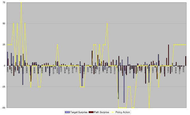
For details, refer to the text immediately following Figure 1.

Supporting Data for Figure 1

Date	Policy Action	Target Surprise	Path Surprise
2/4/1994	25	16.3	8.406135194
3/22/1994	25	0	-4.403796777
4/18/1994	25	15	2.059330804
5/17/1994	50	11.1	-11.98108237
7/6/1994	0	-5	4.108494029
8/16/1994	50	12.4	-5.634277977
9/27/1994	0	-9	5.118326674
11/15/1994	75	12	-2.433294712
12/20/1994	0	-22.6	13.95175767
2/1/1995	50	6.2	3.480962623
3/28/1995	0	-1	3.098661384
5/23/1995	0	0	0.596203223
7/6/1995	-25	-11.2	-18.77626537
8/22/1995	0	3.4	3.887845475
9/26/1995	0	3	4.088828739
11/15/1995	0	4	1.586370578
12/19/1995	-25	-9	1.118326674
1/31/1996	-25	-3	-1.896422293
3/26/1996	0	1	1.093745062
5/21/1996	0	0	2.596203223
7/3/1996	0	-7.2	3.213901984
8/20/1996	0	-2.8	3.003086074
9/24/1996	0	-12	-1.374298842
11/13/1996	0	-1.8	-1.499372087
12/17/1996	0	1.1	-0.956500755
2/5/1997	0	-3.7	5.45529842
3/25/1997	25	4	5.086370578
5/20/1997	0	-9.9	0.57053902
7/2/1997	0	-2.1	1.651365362
8/19/1997	0	0	2.096203223
9/30/1997	0	0	1.096203223
11/12/1997	0	-4.2	-0.7934725
12/16/1997	0	0	-0.403796777
2/4/1998	0	0	3.096203223
3/31/1998	0	-1	1.098661384
5/19/1998	0	-2.6	0.402594442
7/1/1998	0	-0.5	1.347432304
8/18/1998	0	1.2	-0.506746571
9/29/1998	-25	5	-0.416087584
10/15/1998	-25	-24.2	-14.74430927
11/17/1998	-25	-6.9	3.063164536
12/22/1998	0	0	0.596203223
2/3/1999	0	0.6	0.794728326
3/30/1999	0	-1	-2.401338616
5/18/1999	0	-1.2	17.69915302
6/30/1999	25	-3	-9.896422293
8/24/1999	25	3.5	-3.662400342
10/5/1999	0	-4.2	12.7065275
11/16/1999	25	7.5	2.827767013
12/21/1999	0	1.6	4.792270165
2/2/2000	25	-5.9	6.060706374
3/21/2000	25	-4.7	3.457756581
5/16/2000	50	4.1	3.036124762
6/28/2000	0	-2.5	-1.647651374
8/22/2000	0	-1.7	4.450382097
10/3/2000	0	0	7.096203223
11/15/2000	0	-1	1.098661384
12/19/2000	0	6.5	-2.669774825
1/3/2001	-50	-39.3	11.34280896
1/31/2001	-50	3.5	-5.662400342
3/20/2001	-50	7.1	-11.97124972
4/18/2001	-50	-43.8	-5.896129313
5/15/2001	-50	-9.7	-11.02995261
6/27/2001	-25	10.5	1.320392529
8/21/2001	-25	1.6	-4.707729835
10/2/2001	-50	-3.7	-3.54470158
11/6/2001	-50	-15	-8.866924358
12/11/2001	-25	-0.8	-9.501830248
1/30/2002	0	2.5	2.34005782
3/19/2002	0	-2.6	-6.097405558
5/7/2002	0	0.7	-5.75551749
6/26/2002	0	0	1.096203223
8/13/2002	0	4.3	-21.06436687
9/24/2002	0	2	-3.4087131
11/6/2002	-50	-20	1.645366448
12/10/2002	0	0	4.596203223
1/29/2003	0	1	5.593745062
3/18/2003	0	2.4	-2.109696364
5/6/2003	0	3.7	-15.76289197
6/25/2003	-25	13.5	5.813018046
8/12/2003	0	0	-7.403796777
9/16/2003	0	1.1	-0.956500755
10/28/2003	0	-0.5	-12.6525677
12/9/2003	0	0	9.096203223
1/28/2004	0	0.5	24.84497414
3/16/2004	0	0	-9.403796777
5/4/2004	0	-1.2	3.199153016
6/30/2004	25	-0.5	-0.652567696
8/10/2004	25	0.7	4.24448251
9/21/2004	25	0	-1.403796777
11/10/2004	25	-0.8	-4.001830248
12/14/2004	25	-0.9	-0.951584432
2/2/2005	25	0	-1.403796777
3/22/2005	25	0	11.09620322

Footnotes

1. Andersen, Bollerslev, Diebold, and Vega (2003) and Faust, Rogers, Wang, and Wright (2006) examine the effect of FOMC announcement surprises on exchange rates of major currencies against the dollar. Johnson and Jensen (1993), Ehrmann and Fratzcher (2002, 2006), Ehrmann, Fratzcher, and Rigobon (2005) and Wongswan (2005, 2006) examine the effect of FOMC announcements on foreign equity indexes. Robitaille and Roush (2006) examine the effect of FOMC announcements on Brazil's sovereign credit spreads and equity market index. Return to text

2. See details in Section 2. Return to text

3. Krueger and Kuttner (1996) show that fed funds futures contracts yield efficient forecasts of the future fed funds rate. Return to text

4. We use two measures of path surprise. The above defines Path Surprise II. See details in Section 2. Return to text

5. We also use other proxies for financial integration that have been used in the literature. See details in Section 2. Return to text

6. For FOMC meetings that occur in the last seven days of the month, the target surprise is computed as the unadjusted change in the next-month fed funds futures contract. This is to avoid using a very large adjustment factor in the computation of the target surprise which could magnify changes in bid-ask spreads or other factors. Results are qualitatively similar when we compute the target surprise using a one-hour window around the announcement (fifteen minutes before to forty-five minutes after). Return to text

7. For the 94 FOMC meetings in our sample, the estimated equation is $Path\;Surprise\;I_t =-0.64+0.49\ast TS_t$ , and the adjusted R-squared is 0.27. Return to text

8. Interest rate data for Finland and Spain are from Thompson Datastream. Return to text

9. We exclude eight observations from our sample. 1) Mexico, 20 December 1994: The Tequila crisis began; the Mexican peso depreciated 13.7 percent against the dollar. 2) Mexico, 1 February 1995: A U.S. loan package to Mexico was announced; the Mexican peso strengthened 6.7 percent against the dollar. 3) Brazil, 12 November 1997: Fall out from the Asian crisis lead the Brazilian stock market to fall 10.8 percent. 4) Thailand, 2 July 1997: The day after the Bank of Thailand abandoned the baht's peg. The Thai stock market rose 8.3 percent, and in a retracing of the previous days move, the baht appreciated 3.7 percent against the dollar. 5) Korea, 16 December 1997: The Korean government sold 2 banks and issued 10 billion dollars of sovereign bonds. The won depreciated 3.9 percent against the dollar. 6) Indonesia, 19 May 1998: President Suharto announced that he would step down; unrest continued. The Rupiah appreciated 8 percent against the dollar. 7) China, 30 June 1999: There were rumors that premier Zhu Ronji would resign; the stock market fell 7.9 percent. 8) Russia, 17 August 1998: Russia announced a de facto devaluation by widening the trading band of the ruble. Russia also declared its intention to restructure all official domestic currency debt obligations due at the end of 1999 and imposed a 90-day moratorium on the repayment of private external debt. Return to text

10. In our sample, a few FOMC announcements occur before 1 p.m. eastern time. In this case some European equity markets were open at the time of the announcement. Likewise, some late FOMC announcements occurred after the close of some equity markets in Latin America. To account for these special cases, we carefully construct data on the closing time of each equity market in our sample, adjusting for daylight savings time conventions as needed. Return to text

11. Using high-frequency data on 12 foreign ETFs, Bauer and Vega (2005) find significant evidence that private information about U.S. monetary policy plays a role in explaining the cross section of international equity returns at daily and weekly frequencies. Return to text

12. Trade and GDP data for Taiwan come from the CEIC Asia database. Return to text

13. We do not use official liberalization dates (e.g., regulation changes, the introduction of depositary receipts and country funds, or structural breaks in equity capital flows) to proxy for financial integration because most emerging markets liberalized their markets in the late 1980s or the early 1990s, before our sample begins (Bekaert and Harvey (2000) and Henry (2000a, b)). Return to text

14. We obtain Shambaugh's exchange rate classification through 2004 from his webpage. Return to text

15. Alternatively, standard errors can be computed using White's robust standard errors. The empirical results are qualitatively very similar to those obtained from bootstrap standard errors. Return to text

16. Hong Kong's base rate moves exactly one-to-one with the change in the fed funds rate. Return to text

17. The sign effect of target surprise on exchange rates is not robust since the direction of the asymmetry depends on the measure of path surprise. Return to text

18. We use averages over 2001 through 2004 for Foreign Equity Participation and Total Foreign Participation. Return to text

19. Results are qualitatively very similar when we use Path Surprise II. Return to text

20. We use the coarse classification version of Reinhart and Rogoff (2002). We define fixed exchange rate regime (D = 2) as exchange rate regime that was assigned a value of 1 in Reinhart and Rogoff (2002) (e.g., peg, de facto peg, and pre-announced horizontal band that is narrower than or equal to +/- 2 percent), moderately flexible exchange rate regime (D = 1) as an exchange rate regime that was assigned a value of 2 (e.g., pre-announced crawling peg, de facto crawling peg, and pre-announced crawling band that is narrower than or equal to +/- 2 percent), and fully floating (D = 0) as an exchange rate regime that was assigned values of 3 through 6 (e.g., pre-announced crawling band that is wider than or equal to +/- 2 percent, managed floating, freely floating, and falling floating). The data are available through 2001. Return to text

This version is optimized for use by screen readers. Descriptions for all mathematical expressions are provided in LaTex format. A printable pdf version is available. Return to text