
Board of Governors of the Federal Reserve System
International Finance Discussion Papers
Number 897r (June 2007), revised May 2010 --- Screen Reader
Version*
Oil Shocks and External Adjustment **
NOTE: International Finance Discussion Papers are preliminary materials circulated to stimulate discussion and critical comment. References in publications to International Finance Discussion Papers (other than an acknowledgment that the writer has had access to unpublished material) should be cleared with the author or authors. Recent IFDPs are available on the Web at http://www.federalreserve.gov/pubs/ifdp/. This paper can be downloaded without charge from the Social Science Research Network electronic library at http://www.ssrn.com/.
Abstract:
In a two country DSGE model, a shock that raises the price of oil persistently, e.g. an oil supply shock, leads to a deterioration in the oil balance of an oil importing country, such as the United States. With a low oil price elasticity and incomplete financial markets, the increased transfers to the oil exporter are substantial and generate a powerful drag on wealth for the oil importer. This wealth effect is principally responsible for compressing consumption and investment, an exchange rate depreciation, and a surplus in the nonoil balance.
Keywords: Oil-price shocks, trade, DSGE models
JEL classification: F32, F41
1 Introduction
In reaction to the oil crises of the 1970s and early 1980s, as well as the more recent runup in oil prices that started in 2003, the oil component of the U.S. trade balance consistently deteriorated, as can be seen in Figure 1. However, the link between oil prices and the overall goods trade balance appears more elusive. For example, although the overall trade deficit has expanded as oil prices have risen in recent years, it showed some improvement after both the first and second OPEC oil price shocks.
The lack of a close relationship between oil prices and the overall goods trade balance may reflect several factors: other shocks have occurred simultaneously with oil shocks, oil shocks markedly affect the nonoil balance through general equilibrium channels, and each shock may be associated with a different transmission channel. We explore these issues with a dynamic stochastic general equilibrium model.
Our model builds on the work of [Backus and Crucini 1998]. Each of the two countries in our model produces a distinct good that is used as an input into the production of consumption and investment both at home and abroad. Oil serves as an input into the production of the domestic good, and also enters directly into the household consumption bundle. One country is an oil importer, while the other is an oil exporter. However, the model differs importantly from that of [Backus and Crucini 1998] along two dimensions. To emphasize the role of both differential wealth effects across countries and substitution effects in the transmission of oil shocks, we depart from their complete markets framework by assuming that only one non state-contingent bond is traded across countries. In addition, while [Backus and Crucini 1998] focused on oil supply and technology shocks as drivers of oil price fluctuations, in line with recent empirical evidence by [Kilian 2009] and [Kilian et al. 2009], we include oil demand shocks. 1
We gauge the relative importance of the various shocks by matching key moments in the model to corresponding moments in U.S. data. At medium-run frequencies, oil demand and supply shocks account half of the variation in the nonoil balance.2 However, these shocks account for only one sixth of the variation in the overall goods trade balance, pointing towards sizable general equilibrium effects.
As documented in the next section, the literature that modeled the effect of oil shocks can be divided into two broad categories, depending on whether the focus was on a closed or an open economy setting. The closed economy treatment of the subject has abstracted from the fact that many economies import oil from abroad in order to emphasize either the allocative effects on different industries or the intertemporal production choices involved when the price of the oil input changes exogenously. By contrast, much of the open economy work has focused on differential cross-country wealth effects and has modeled oil price shocks as changes in transfer payments across countries.
The model in this paper bridges the gap between the open and closed economy strands of the literature. Following the closed economy approach, the model links the dynamic investment and saving decisions to the choice of factor inputs in production explicitly. Moreover, following the open economy literature, the model keeps track of relative wealth effects across countries.3
We illustrate the general equilibrium repercussions of a change in the price of oil by focusing first on a contraction in the foreign oil supply. For an oil importer, such as the United States, producers and households substitute away from oil. Nonetheless, the oil component of the trade balance deteriorates but the nonoil component of the trade balance improves. This improvement in the nonoil component is attributable to a negative wealth effect on the oil importer relative to the oil exporter, which induces the former's nonoil terms of trade to worsen, and its nonoil imports to contract. Accordingly, the response of the overall goods trade balance is dampened.
Key features that impact the relative wealth effects across countries are the degree of substitutability between oil and other production factors, the relative oil endowment, and the degree of international risk-sharing. A lower oil price elasticity of demand implies that an oil importer runs a larger deficit on the oil component of its trade balance. In turn, the larger oil deficit requires a larger nonoil trade surplus, and a further worsening of the nonoil terms of trade. Similarly, with a smaller oil endowment, the oil importer experiences a larger deterioration in the terms of trade. Finally, enhanced international risk-sharing reduces the need to counterbalance oil deficits with nonoil trade surpluses and dampens the associated fluctuations in the terms of trade, but enhances the fluctuation in the overall goods trade balance.
For oil shocks, the responses derived in our framework under complete financial markets, incomplete markets, and financial autarky are distinct from each other. This result stands in contrast with the typical finding for technology shocks when traded goods are sufficiently substitutable.4 In that case, as noted by [Cole and Obstfeld 1991], movements in the terms of trade are a powerful source of insurance against technology shocks independently of the available set of assets. Under a low elasticity of substitution between traded goods, as pointed out by [Corsetti et al. 2008], a positive technology shock abroad causes the home country's terms of trade to worsen. In our model, the home country's terms of trade also worsen (and the real exchange rate depreciates) after a contractionary shock to foreign oil supply. Hence, in both [Corsetti et al. 2008] and our contribution, the terms of trade fail to provide insurance and pronounced differences between the complete markets case and the incomplete markets setting can occur.
Our work also bridges the gap between the latest empirical evidence on the sources of oil price movements and DSGE models (which have typically taken oil prices as exogenous). With an endogenous oil price, we highlight commonalities and differences across several source of fluctuation: oil supply shocks, oil demand shocks, and technology shocks.
Foreign oil demand shocks, modeled as shocks that affect the efficiency of oil inputs in production and consumption, eventually induce similar effects to those of foreign supply disturbances. However, their initial dynamics differ substantially. The moment matching exercise calls for a strong growth component for the shocks (as well as a slow-reverting error-correction component for the level) that induces rising oil prices over an extended period when efficiency contracts and oil demand expands. Since the shock lowers foreign activity disproportionately, the improvement in the nonoil balance is delayed.
In the case of technology shocks, the increase in the oil bill is not the main force influencing external adjustment. The typical effects of a technology shock dominate oil market considerations. With a trade elasticity close to one, the increase in foreign production stimulates home export demand in spite of an appreciation of the home exchange rate. Both the nonoil and the overall goods trade balance improve drastically, notwithstanding the deterioration in the oil balance.
The rest of the paper proceeds as follows: Section 2 reviews the literature on oil shocks, Sections 3 describes the model, Section 4 outlines the calibration and moment matching exercise, Sections 5 and 6 illustrate the model through numerical simulations, and Section 7 concludes.
2 Literature Review
Since the large fluctuations in the relative price of oil in the 1970s, a large and growing literature has examined the macroeconomic effects of oil shocks and the channels through which oil shocks operate. A first set of papers tackled the question with empirically-justified models and the principal aim to size the oil-price/GDP elasticity. A second set of papers interpreted the empirical findings that pointed to large macroeconomic effects of oil shocks through the lens of structural models.5
Early empirical studies such as [Rasche and Tatom 1977] regressed GDP on oil prices and other control variables. Subsequent work, starting with [Hamilton 1983], addressed potential endogeneity issues, settling on a censored measure of oil price increases, and singling out episodes of rapidly rising prices.6
[Barsky and Kilian 2004] reviewed the arguments linking oil price increases to lower economic growth and provided arguments in favor of reverse causality from macroeconomic variables to oil prices. [Kilian 2009] pioneered a way to decompose oil price movements into three components driven by shocks to oil supply, global activity, and oil demand.7 [Cavallo and Wu 2009] propose a novel method of measuring oil price shocks that relies on narrative evidence from oil industry publications.
General equilibrium models are ideally suited to control for reverse causality. The literature that used structural models can be divided into two categories, depending on whether the focus was on a closed or open economy setting. The closed economy treatment has emphasized either the allocative effects on different industries or the intertemporal production choices when the price of an input suddenly changes at the cost of abstracting from the fact that many economies import oil from abroad. By contrast, much of the open economy work focused on wealth effects associated with the redistribution of income between oil importers and exporters after oil price changes.
Early contributions with a closed economy focus include [Pierce et al. 1974] who used the MPS (MIT-Penn-SSRC) econometric model to obtain quantitative estimates on individual sectors of the U.S. economy for the effects of a permanent rise in in the price of oil.8 While the early models were rich in sectoral detail, they did not link the optimal choice of factor inputs in production to intertemporal saving and consumption decisions. [Kim and Loungani 1992] solved this shortcoming by extending the real business cycle model of [Kydland and Prescott 1982] to include oil inputs in the production function.9 [Leduc and Sill 2004] augmented the model of [Kim and Loungani 1992] to tackle the question originally raised in the VAR study by [Bernanke et al. 1997] of how alternative monetary policy specifications influence the transmission of oil shocks.10
Early open economy contributions include [Schmid 1976], [Findlay and Rodriguez 1977], and [Buiter 1978]. None of these contributions tackled the intertemporal decision on savings and investment. [Svensson 1984] examined the welfare effects and the trade balance response to changes in the world oil prices for a small oil-importing economy in the context of a two-period model.
In the related literature on the wealth effects of a domestic resource discovery, or "Dutch Disease", [Bruno and Sachs 1982a] used a dynamic model with infinitely lived agents, while taking the world rate of interest, foreign prices, and foreign wealth as exogenous. The model extended the principally static analysis of earlier contributions by allowing for short-run capital specificity and long-run capital mobility, international capital flows, far-sighted intertemporal optimizing behavior of households and firms.11
Building on the Dutch disease literature, [Wijnbergen 1984] and [Krugman 1987] developed dynamic open economy models of endogenous growth. However, the production function only incorporated labor. Both [Wijnbergen 1984] and [Krugman 1987] modeled oil price shocks as transfer payments across countries, capturing country-specific wealth effects, but not the substitution effects for factor inputs, a key feature of the closed economy studies.
The model in this paper bridges the gap between the open and closed economy strands of the literature. Following the closed economy approach, the model links the dynamic investment and saving decisions to the choice of factor inputs in production explicitly. Moreover, following the open economy approach, the model keeps track of changes in wealth across countries.12
3 Model Description
There are two countries, a home country (calibrated based on U.S. data) and a foreign country (rest-of-the-world). Because the structure of the country blocs is symmetric, we focus on the home country, although our calibration allows for differences in population size and in the per capita oil endowment. Each country specializes in the production of a final good that is an imperfect substitute for the final good produced in the other country. Production requires capital, labor, and oil. The investment bundle is a composite of the domestically produced good and inputs of the foreign good. The consumption bundle is a composite of the domestically produced good, imports of the foreign good, and oil. For expositional purposes, the consumption bundle is assumed to be produced by a competitive distribution sector with a productive structure that mirrors household preferences over the three goods. While asset markets are complete at the country level, asset markets are incomplete internationally. Finally, both the home and foreign country are endowed with a non-storable supply of oil each period.
3.1 Households
The utility functional of a typical member of household
![]() is
is
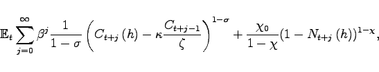 |
(1) |
where the discount factor ![]() satisfies
satisfies![]() The period utility function
depends on an individual's current and lagged consumption, where
The period utility function
depends on an individual's current and lagged consumption, where
![]() parameterizes the extent of external
habit persistence in consumption. The period utility function also
depends on leisure,
parameterizes the extent of external
habit persistence in consumption. The period utility function also
depends on leisure,
![]() . Population
differences across countries are captured by
. Population
differences across countries are captured by ![]() , the household size in the home country, while we
normalize household size in the foreign country to unity.
, the household size in the home country, while we
normalize household size in the foreign country to unity.
Each member of household ![]() faces a budget
constraint in period
faces a budget
constraint in period ![]() which states that the
combined expenditure on goods and the net accumulation of financial
assets must equal disposable income:
which states that the
combined expenditure on goods and the net accumulation of financial
assets must equal disposable income:
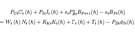 |
(2) |
Final consumption goods are purchased at the price ![]() and final investment goods at the price
and final investment goods at the price ![]() Investment in physical capital augments the per capita
capital stock
Investment in physical capital augments the per capita
capital stock ![]() according to a linear
transition law of the form:
according to a linear
transition law of the form:
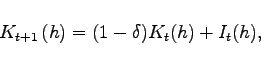 |
(3) |
Individuals accumulate financial assets by purchasing
state-contingent domestic bonds, and a non state-contingent foreign
bond. Given the representative agent structure at the country
level, we omit terms involving the former from the budget
constraint. The term ![]() in the budget
constraint represents the quantity of the non state-contingent bond
purchased by a typical member of household
in the budget
constraint represents the quantity of the non state-contingent bond
purchased by a typical member of household ![]() at time
at time
![]() that pays one unit of foreign currency in
the subsequent period,
that pays one unit of foreign currency in
the subsequent period,
![]() is the foreign currency price
of the bond, and
is the foreign currency price
of the bond, and ![]() is the exchange rate expressed in
units of home currency per unit of foreign currency. To ensure that
net foreign assets are stationary, we follow [Turnovsky 1985] and
assume there is an intermediation cost
is the exchange rate expressed in
units of home currency per unit of foreign currency. To ensure that
net foreign assets are stationary, we follow [Turnovsky 1985] and
assume there is an intermediation cost ![]() paid
by households in the home country for purchases of foreign bonds.
Specifically, the intermediation costs depend on the ratio of
economy-wide holdings of net foreign assets to nominal output
(
paid
by households in the home country for purchases of foreign bonds.
Specifically, the intermediation costs depend on the ratio of
economy-wide holdings of net foreign assets to nominal output
(![]() , defined below):
, defined below):
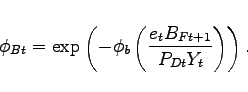 |
(4) |
If the home economy has an overall net lender position, a household will earn a lower return on any holdings of foreign bonds. By contrast, if the economy has a net debtor position, a household will pay a higher return on any foreign debt.
Each member of household ![]() earns labor income
earns labor income
![]() and
capital income
and
capital income
![]() . The member also receives an
aliquot share
. The member also receives an
aliquot share
![]() of the sum of firm
profits and the sale of oil services, and receives net transfers of
of the sum of firm
profits and the sale of oil services, and receives net transfers of
![]() . Finally, as in [Christiano
et al. 2005], it is costly to change the level of gross
investment from the previous period, so that the acceleration in
the capital stock is penalized:
. Finally, as in [Christiano
et al. 2005], it is costly to change the level of gross
investment from the previous period, so that the acceleration in
the capital stock is penalized:
 |
(5) |
In every period ![]() , a typical member of
household
, a typical member of
household ![]() maximizes the utility functional
(1) with respect to consumption,
labor supply, investment, end-of-period capital stock, and holdings
of foreign bonds, subject to its budget constraint (2), and the transition equation for capital
(3). In doing so, prices, wages, and net
transfers are taken as given.
maximizes the utility functional
(1) with respect to consumption,
labor supply, investment, end-of-period capital stock, and holdings
of foreign bonds, subject to its budget constraint (2), and the transition equation for capital
(3). In doing so, prices, wages, and net
transfers are taken as given.
Firms and Production
Each country produces a single distinct nonoil good. Focusing on the home country, this nonoil good is produced by perfectly competitive firms according to a constant-returns-to-scale technology. The representative firm's technology can be characterized as a nested constant-elasticity of substitution specification of the form:
 |
(6) |
 |
(7) |
Each producer utilizes capital and labor services, ![]() and
and ![]() , to make a " value-added"
input
, to make a " value-added"
input ![]() . This composite input is combined with
oil services
. This composite input is combined with
oil services ![]() to produce the domestic nonoil good
to produce the domestic nonoil good
![]() . The term
. The term ![]() represents
a stochastic process for the evolution of technology. The term
represents
a stochastic process for the evolution of technology. The term
![]() represents a stochastic process for
the oil intensity in production, which might capture a switch in
the composition of capital towards machines with different energy
intensities.
represents a stochastic process for
the oil intensity in production, which might capture a switch in
the composition of capital towards machines with different energy
intensities.
The representative producer chooses a contingency plan for
![]() ,
, ![]() , and
, and ![]() that minimizes the cost of producing the domestic
output good subject to equations (6) and
(7). In solving this problem, the producer
takes as given the rental price of capital
that minimizes the cost of producing the domestic
output good subject to equations (6) and
(7). In solving this problem, the producer
takes as given the rental price of capital ![]() , the
wage
, the
wage ![]() , and the price of oil
, and the price of oil ![]() . The representative firm sells its output to households
and firms at a price
. The representative firm sells its output to households
and firms at a price ![]() , which is the Lagrange
multiplier from the cost-minimization problem.
, which is the Lagrange
multiplier from the cost-minimization problem.
Production of Consumption and Investment Goods
The consumption basket ![]() that enters the
household's budget constraint can be regarded as produced by
perfectly competitive consumption distributors. The form of the
production function mirrors the preferences of households over
consumption of nonoil goods and oil. These distributors purchase a
nonoil consumption good
that enters the
household's budget constraint can be regarded as produced by
perfectly competitive consumption distributors. The form of the
production function mirrors the preferences of households over
consumption of nonoil goods and oil. These distributors purchase a
nonoil consumption good ![]() and oil services
and oil services
![]() as inputs in perfectly competitive
input markets, and produce a composite consumption good according
to a CES production function:
as inputs in perfectly competitive
input markets, and produce a composite consumption good according
to a CES production function:
 |
(8) |
where the quasi-share parameter ![]() determines the importance of oil purchases in the household's
composite consumption bundle, and the parameter
determines the importance of oil purchases in the household's
composite consumption bundle, and the parameter ![]() determines the long-run price elasticity of demand
for oil. The term
determines the long-run price elasticity of demand
for oil. The term ![]() represents a
stochastic process for the oil intensity in the production of the
consumption bundle. This shock could capture changes in oil demand
coming from external factors, such as unusually cold winters, or a
shift towards consuming goods that are more energy intensive.
represents a
stochastic process for the oil intensity in the production of the
consumption bundle. This shock could capture changes in oil demand
coming from external factors, such as unusually cold winters, or a
shift towards consuming goods that are more energy intensive.
Consumption distributors choose a contingency path for their
inputs ![]() and
and ![]() to minimize the
costs of producing the consumption bundle, taking as given input
prices
to minimize the
costs of producing the consumption bundle, taking as given input
prices ![]() and
and ![]() , respectively.
The Lagrangian multiplier from this cost-minimization problem
determines the price of the consumption bundle charged to
households, i.e.,
, respectively.
The Lagrangian multiplier from this cost-minimization problem
determines the price of the consumption bundle charged to
households, i.e., ![]() in the household's
budget constraint given in equation (2).
in the household's
budget constraint given in equation (2).
Similarly, the nonoil consumption good ![]() and
investment good
and
investment good ![]() are produced by perfectly
competitive distributors. Both the domestically produced nonoil
good and the foreign nonoil good are utilized as inputs, though we
allow for the proportion of each input to differ between nonoil
consumption and investment goods. The production function for the
nonoil consumption good
are produced by perfectly
competitive distributors. Both the domestically produced nonoil
good and the foreign nonoil good are utilized as inputs, though we
allow for the proportion of each input to differ between nonoil
consumption and investment goods. The production function for the
nonoil consumption good ![]() is given by:
is given by:
 |
(9) |
where ![]() denotes the quantity of the
domestically-produced nonoil good purchased at a price of
denotes the quantity of the
domestically-produced nonoil good purchased at a price of
![]() , and used as an input by the
representative nonoil consumption distributor. The term
, and used as an input by the
representative nonoil consumption distributor. The term ![]() denotes imports of the foreign nonoil good purchased at
a price of
denotes imports of the foreign nonoil good purchased at
a price of ![]() . The term
. The term ![]() captures an import preference shock. In the moment matching
exercise that follows, this shock soaks up the volatility of nonoil
goods trade not explained by the remaining shocks. The Lagrangian
multiplier from the cost minimization problem for the distributors
determines the price of the nonoil consumption good,
captures an import preference shock. In the moment matching
exercise that follows, this shock soaks up the volatility of nonoil
goods trade not explained by the remaining shocks. The Lagrangian
multiplier from the cost minimization problem for the distributors
determines the price of the nonoil consumption good, ![]() .
.
Finally, the production function for investment goods is
isomorphic to that given in equation (9),
though allowing for possible differences in the import intensity of
investment goods (determined by ![]() , akin to
, akin to
![]() in equation (9)), and the degree of substitutability between
nonoil imports and domestically-produced goods in producing
investment goods (determined by
in equation (9)), and the degree of substitutability between
nonoil imports and domestically-produced goods in producing
investment goods (determined by ![]() ). The import
preference shock
). The import
preference shock ![]() also affects investment
imports. The Lagrangian from the problem that investment
distributors face determines the price of new investment goods,
also affects investment
imports. The Lagrangian from the problem that investment
distributors face determines the price of new investment goods,
![]() , that appears in the household's budget
constraint.13
, that appears in the household's budget
constraint.13
3.3 The Oil Market
Each period the home and foreign countries are endowed with
exogenous supplies of oil ![]() and
and ![]() , respectively. The two endowments are governed by
distinct stochastic processes.
, respectively. The two endowments are governed by
distinct stochastic processes.
With both domestic and foreign oil supply determined
exogenously, the oil price ![]() adjusts
endogenously to clear the world oil market:
adjusts
endogenously to clear the world oil market:
 |
(10) |
To clear the oil market, the sum of home and foreign oil
production must equal the sum of home and foreign oil consumption
by firms and households. Because all variables are expressed in per
capita terms, foreign variables are scaled by the relative
population size of the home country
![]() , in equation 10.
, in equation 10.
3.4 Fiscal Policy
The government purchases a fixed share ![]() of the
domestic nonoil good
of the
domestic nonoil good ![]() but the import content
of government purchases is zero. Government purchases
but the import content
of government purchases is zero. Government purchases ![]() have no direct effect on household utility. Given
the Ricardian structure of our model, we assume that net lump-sum
transfers
have no direct effect on household utility. Given
the Ricardian structure of our model, we assume that net lump-sum
transfers ![]() are adjusted each period to balance
the government receipts and revenues, so that:
are adjusted each period to balance
the government receipts and revenues, so that:
| (11) |
3.5 Resource Constraints for Nonoil Goods, and Net Foreign Assets
The resource constraint for the nonoil goods sector of the home economy can be written as:
 |
(12) |
where ![]() denotes foreign imports - again
expressed in per capita terms, which accounts for the population
scaling factor
denotes foreign imports - again
expressed in per capita terms, which accounts for the population
scaling factor
![]() . The term
. The term ![]() denotes the resources that are lost due to costs of
adjusting investment.
denotes the resources that are lost due to costs of
adjusting investment.
The evolution of net foreign assets can be expressed as:
 |
(13) |
This expression can be derived by combining the budget constraint for households, the government budget constraint, and the definition of firm profits.
4 Solution Method and Calibration
The model is log-linearized around its steady state.14 To obtain the reduced-form solution of the model, we use the numerical algorithm of [Anderson and Moore 1985], which provides an efficient implementation of the method proposed by [Blanchard and Kahn 1980].15
The model is calibrated at a quarterly frequency. The parameter
values for the home economy under our benchmark calibration are
listed in Table 1. Parameters for
the foreign economy are identical except for the parameters
determining the intensity of oil use, the capital share of
production, and the trade shares. The latter are determined by the
assumption that trade is balanced in the steady state and that the
relative population size, ![]() , is scaled so
that the home economy accounts for one third of world GDP.
, is scaled so
that the home economy accounts for one third of world GDP.
The discount factor ![]() is 0.99. The parameter
is 0.99. The parameter
![]() in the subutility function over
consumption is set equal to 1.5. We set
in the subutility function over
consumption is set equal to 1.5. We set ![]() ,
implying a Frisch elasticity of labor supply of 0.2. The utility
parameter
,
implying a Frisch elasticity of labor supply of 0.2. The utility
parameter ![]() is set so that employment
comprises one-third of the household's time endowment. In line with
[Smets and Wouters 2007], the real rigidities affecting
consumption,
is set so that employment
comprises one-third of the household's time endowment. In line with
[Smets and Wouters 2007], the real rigidities affecting
consumption, ![]() , and investment,
, and investment, ![]() , are 0.8 and 3, respectively.
, are 0.8 and 3, respectively.
The production function parameter ![]() is set
to -2, implying an elasticity of substitution between capital and
labor of 0.5. The depreciation rate of capital
is set
to -2, implying an elasticity of substitution between capital and
labor of 0.5. The depreciation rate of capital ![]() is consistent with an annual depreciation rate
of 10 percent. We set the government share of output to 18 percent,
and adjust the quasi-capital share parameter
is consistent with an annual depreciation rate
of 10 percent. We set the government share of output to 18 percent,
and adjust the quasi-capital share parameter ![]() , so that the investment share of output equals an
empirically-realistic value of 20 percent.
, so that the investment share of output equals an
empirically-realistic value of 20 percent.
Our calibration of ![]() and
and ![]() is determined by the overall oil share of output,
and the end-use ratios of oil in consumption and production. Based
on data from the Energy Information Administration of the U.S.
Department of Energy for 2008, the overall oil share of the
domestic economy is set to 4.2 percent, with one-third of total oil
usage accounted for by households, and two-thirds by firms. The oil
imports of the home country are set to 70 percent of total demand
in the steady state, implying that one third of oil demand is
satisfied by domestic production. This estimate is based on 2008
data from the National Income and Product Accounts. In the foreign
block, the overall oil share is set to 8.2 percent. The oil
endowment abroad is 9.5 percent of foreign GDP, based on oil supply
data from the Energy Information Administration.
is determined by the overall oil share of output,
and the end-use ratios of oil in consumption and production. Based
on data from the Energy Information Administration of the U.S.
Department of Energy for 2008, the overall oil share of the
domestic economy is set to 4.2 percent, with one-third of total oil
usage accounted for by households, and two-thirds by firms. The oil
imports of the home country are set to 70 percent of total demand
in the steady state, implying that one third of oil demand is
satisfied by domestic production. This estimate is based on 2008
data from the National Income and Product Accounts. In the foreign
block, the overall oil share is set to 8.2 percent. The oil
endowment abroad is 9.5 percent of foreign GDP, based on oil supply
data from the Energy Information Administration.
Turning to the parameters determining trade flows, the parameter
![]() is chosen to match the estimated
average share of imports in total U.S. consumption of about 7
percent using NIPA data, while the parameter
is chosen to match the estimated
average share of imports in total U.S. consumption of about 7
percent using NIPA data, while the parameter ![]() is chosen to match the average share of imports in
total U.S. investment of about 40 percent. This calibration implies
a ratio of nonoil goods imports relative to GDP for the home
country of about 12 percent. Given that trade is balanced in steady
state, and that the oil import share for the home country is 3
percent of GDP, the goods export share is 15 percent of GDP.
is chosen to match the average share of imports in
total U.S. investment of about 40 percent. This calibration implies
a ratio of nonoil goods imports relative to GDP for the home
country of about 12 percent. Given that trade is balanced in steady
state, and that the oil import share for the home country is 3
percent of GDP, the goods export share is 15 percent of GDP.
4.1 Moment Matching
The parameters governing the elasticity of substitution for oil,
![]() , the elasticity of substitution
between domestic and foreign goods,
, the elasticity of substitution
between domestic and foreign goods, ![]() ,
and the autoregressive processes for the various shocks in the
model are calibrated using the simulated method of moments. The oil
demand shocks in consumption and production are constrained to be
identical in each country, i.e.,
,
and the autoregressive processes for the various shocks in the
model are calibrated using the simulated method of moments. The oil
demand shocks in consumption and production are constrained to be
identical in each country, i.e.,
![]() .16 Accordingly, the
model incorporates 4 shock processes in each of the 2 countries:
technology shocks, import preference shocks, oil supply shocks, and
oil demand shocks. The first three types of shocks are governed by
an AR(1) process. However, the oil demand shock is governed by an
AR(2) process that captures a growth rate component and imposes an
error correction term to ensure stationarity in levels.17 We
constrain the auto-regressive parameters to be identical in the
U.S. and the foreign bloc, but left the standard deviations of the
innovations unconstrained. We assume that the innovations to all
the other shock processes are independent of each other. The
calibration procedure involves minimizing the square of the
distance between key moments generated from the model and their
observed counterparts.
.16 Accordingly, the
model incorporates 4 shock processes in each of the 2 countries:
technology shocks, import preference shocks, oil supply shocks, and
oil demand shocks. The first three types of shocks are governed by
an AR(1) process. However, the oil demand shock is governed by an
AR(2) process that captures a growth rate component and imposes an
error correction term to ensure stationarity in levels.17 We
constrain the auto-regressive parameters to be identical in the
U.S. and the foreign bloc, but left the standard deviations of the
innovations unconstrained. We assume that the innovations to all
the other shock processes are independent of each other. The
calibration procedure involves minimizing the square of the
distance between key moments generated from the model and their
observed counterparts.
Following [Comin and Gertler 2006], we bandpass filtered the data used in estimation to retain only oscillations with amplitude between 6 and 200 quarters.18 Going beyond business cycle frequencies avoids the exclusion of nearly permanent movements or slow-moving adjustments that are important ingredients in understanding fluctuations in the trade balance. Oil shocks may cause slow interactions between the nonoil balance and oil imports that are of principal interest in this exercise. However, we also report the implications of our calibration for moments at business cycle frequencies.
The distance function for the moment matching exercise includes the standard deviation and the first-order autocorrelation of eight variables: U.S. and foreign GDP, U.S. and foreign oil supply, the relative price of oil, and oil imports, nonoil goods imports, and the overall goods trade balance expressed as a share of GDP.19 In an attempt to normalize the various moments included in the distance function, we scaled them by the size of the corresponding moment in the data. Table 2 reports the parameter values that minimized the distance function. The calibration of the elasticity of substitution for oil, at a value of 0.38, is in line with previous empirical estimates.20The value for the goods trade elasticity, at 1.1 is in line with typical estimates using aggregate data.21
The moments underlying the distance function are reported in Tables 3 and 4. The model matches the moments in the data closely. Table 3 shows that oil shocks play essentially no role in accounting for the volatility of U.S. output at medium-run frequencies (encompassing oscillations with amplitude from 6 to 200 quarters). By contrast, at these frequencies, the bulk of the volatility in the oil price and in the oil import share are explained by oil demand and supply shocks, with oil demand shocks playing a larger role. Moreover, about half of the variation in the nonoil balance is attributed to oil shocks. Because of offsetting effects between the nonoil balance and oil imports, oil shocks account for a more modest fraction of the volatility in the overall goods trade balance.
Finally, Table 5 reports the variance at business cycle frequencies (including oscillations with amplitude from 6 to 32 quarters) for the variables in the distance function, keeping the calibration unvaried. Remarkably, the model still comes close to replicating the observed variances; the only large miss is the variance for the oil price. At business cycle frequencies, productivity shocks explain again most of the variation in GDP and oil shocks explain most of the variation in oil prices. These findings are in line with those reported in [Backus and Crucini 1998], notwithstanding their omission of oil demand shocks.
5 Model Simulations
We start by reporting simulation results for oil supply shocks. This approach is in the spirit of much of the previous literature, which analyzed the effects of oil price fluctuations that were ascribed exclusively to supply shocks. In addition, a focus on supply shocks facilitates the exploration of wealth and substitution effects, as these shocks lead to nearly permanent increases in the price of oil in our calibrated model. In Section 6, we highlight commonalities and differences between oil supply shocks, oil demand shocks, and technology shocks.
Figure 2 shows responses of the home oil-importing country under our benchmark calibration. The shock reduces foreign oil supply and is scaled at standard deviations. The resulting 8 percent persistent rise in the price of oil induces a fall in home oil demand. Both households and firms substitute away from the more costly oil input. Given an elasticity of oil demand around 0.4, demand drops about 3 percent.
The decline in oil use has effects on gross nonoil output, the expenditure components, and the real interest rate that resemble those of a highly persistent decline in productivity. Lower oil use leads to a fall in the current and future marginal product of capital, causing investment and gross output to fall. In the long term the capital stock also falls. Consumption contracts due to a reduction in household income. The real interest rate falls, notwithstanding a transient initial increase due to habit formation in preferences.
Turning to the implications for the external sector, the drop in domestic oil demand translates into a 4.5 percent fall of real oil imports, as the home country imports about two thirds of its oil use in steady state. Given oil imports amount to about 3 percent of GDP in steady state, the oil balance deteriorates 0.1 percentage point (equal to the drop in imports times its share of GDP, net of the oil price increase).
While the responses of consumption output and investment to the oil supply shock resemble those of a persistent contraction in technology, the exchange rate response does not.22 Since the rational expectations solution requires that the net foreign asset position is bounded away from infinity (conditional on current information), the home country's nonoil balance must improve enough to offset the long-run deterioration in the oil balance, as well as to finance interest payments on the stock of debt accumulated along the transition path. Thus, the exchange rate (the terms of trade track the real exchange rate closely) depreciates, which stimulates home nonoil net exports. As the shock to oil supply leads to a very persistent rise in oil prices, consumption smoothing dictates a quick offset of the deficit from the oil side of the trade balance by a surplus in the nonoil balance. If the offset were delayed, a greater accumulation of debt and related interest rate payments would reduce future consumption inefficiently.
Figure 3 contrasts the responses of the persistent oil supply contraction under our baseline calibration with those of a shock with lower persistence (the AR(1) coefficient is 0.5). With the less persistent shock, the rise in oil prices would be more transient. Consumption smoothing in concert with a smaller depreciation of the exchange rate imply a smaller improvement in the nonoil balance; hence, the overall trade balance deteriorates almost twice as much on impact.
5.1 Key Parameters Influencing the Wealth Effect
If oil demand is sufficiently price-inelastic, a reduction in foreign oil supply raises the present value of oil imports. The resulting deterioration in the overall goods trade balance is offset by an improvement in the nonoil balance. This improvement is attributable to a negative wealth effect on the oil-importing country relative to the foreign oil exporter.
Several structural parameters play a key role in determining the relative wealth effects across countries. Figure 4 contrasts the responses to a foreign oil contraction sized at two standard deviations under our benchmark calibration and under two alternative calibrations of the price elasticity of oil demand. One alternative imposes an elasticity of unity, consistent with a Cobb-Douglas production function over the factor inputs. The other alternative imposes an elasticity of 0.10, close to a Leontief specification.23
With the size of the oil supply disruption kept constant across the cases shown in Figure 4, the oil price rises about four times as much under the near-Leontief specification as under our baseline calibration. As the oil price elasticity of demand under the alternative calibration is about one quarter of the one in the benchmark calibration, home oil demand falls again about 3 percent. However, under the alternative the resulting deterioration of the oil component of the trade balance is considerably larger; the associated transfer of relative purchasing power further depresses home relative to foreign wealth. To obtain a bigger improvement in the nonoil balance, the real exchange rate depreciates by more.
Under the alternative with a unitary price elasticity of demand, real oil demand falls by exactly the same magnitude as the increase in the oil price. Because the home country produces oil, real imports decline by more than the price rises, implying an improvement in the oil balance. With the oil balance improving, the nonoil balance deteriorates.
Figure 4 compares model responses under our benchmark calibration in which the home country has an oil endowment equal to one third of its steady state oil consumption with an alternative in which it has no oil endowment ("no domestic oil production").24 A shock to foreign oil supply sized at two standard deviations induces a larger rise in the price of oil if the home country has to import all of the oil used. Given the larger deficit in the oil component of the trade balance under the case of no domestic oil production, the improvement in the nonoil balance must be larger, which entails a larger depreciation of the real exchange rate.
5.2 Complete vs. Incomplete Markets
In our model, oil shocks affect the dynamics of nonoil variables through changes in wealth across countries. To elucidate the role of such changes, Figure 6 contrasts the responses under our benchmark case with incomplete financial markets to those with complete financial markets and financial autarchy. Under either financial market arrangement, the oil price rises about 8 percent in response to a two-standard-deviation shock that contracts foreign oil supply.
The deterioration in the oil balance is also comparable in magnitude across cases. By contrast, the results for the remaining variables in Figure 6 are strikingly different: in particular, under complete markets the nonoil balance is virtually unchanged from its steady state level and the depreciation of the real exchange rate is substantially reduced.25
Under complete markets, ownership of the profit flow associated with oil production is effectively shared across countries through insurance transfers. These insurance transfers enable the home country to satisfy the intertemporal budget constraint without having to accrue much of a surplus on the nonoil balance. Accordingly, the response of the exchange rate is muted relative to the incomplete market case.
Under financial autarchy, the effects of the shocks cannot be smoothed at all and the real exchange rate depreciates by more so that the deficit in the oil balance can be completely offset by a surplus in the nonoil balance in every period.
The responses under incomplete financial markets resemble those under financial autarchy much more than those under complete markets; this result contrasts sharply with the typical effects of technology shocks that would also obtain in our model. [Baxter and Crucini 1995] showed that for technology shocks the equilibrium allocations in models where agents trade only one non state-contingent international bond are very close to those derived in an economy with complete international financial markets, provided that the technology shock is not permanent. Furthermore, [Cole and Obstfeld 1991] pointed out that movements in the terms of trade provide a powerful source of insurance against technology shocks independently of the set of internationally available assets.26 Thus, in standard models of the international business cycle that focused on technology shocks, the movement in relative prices offsets the wealth effects. A notable exception is [Corsetti et al. 2008]. These authors showed that under a low elasticity of substitution between traded goods, the movement in relative prices operates to reinforce the wealth effects of the shock. Thus, their model implies pronounced differences between the three financial market arrangements (complete markets, one bond economy, and financial autarchy).
In our model, a contractionary shock to oil supply leads to a depreciation of the real exchange rate for the oil importing country. Hence, as in [Corsetti et al. 2008], the exchange rate does not provide insurance to the oil importer. The responses to oil supply shocks continue to differ across the three financial market arrangements even for less persistent shocks to oil supply, although it is not obvious how to aggregate implications across different variables. Similar results obtain for oil efficiency shocks.27
Although we do not model the gross holdings of international assets explicitly, our analysis sheds light on the importance of valuation effects. As discussed by [Kilian et al. 2009], changes in asset prices and the real exchange rate affect the international wealth distribution in response to oil shocks. Positing optimal portfolio allocations, such valuation effects can be thought as yielding additional insurance. The more diversified the countries are, the more effectively they can insure each other against movements in the price of oil, leading to smoother real exchange rates and larger movements of the overall goods trade balance.
5.3 Wealth and Substitution Effects
In the preceding discussion, we have argued heuristically that differences in wealth effects across countries shape the response of the nonoil balance and the real exchange rate. To quantify the wealth effect, and the extent to which it accounts for most of the disparity in the responses of consumption and labor supply across countries, we employ the "Hicksian" decomposition devised by [King 1990].
King's method decomposes the consumption and labor supply responses into (i) a wealth effect, (ii) a real wage effect, and (iii) a real interest rate effect. To compute the wealth effects, we first find the change in discounted lifetime utility due to the oil price shock. As preferences are time-separable, the wealth effects on consumption and labor supply are given by the constant consumption and labor profiles that match the computed change in utility while wages and interest rates are held constant at their steady state values. The real wage effect is the part of the overall response in consumption or labor that is due to changes in the real wage alone, keeping utility at its steady state level. The real interest rate effect is computed analogously.
In Figure 7 we plot the wealth and the two substitution effects for consumption in the home (left panel) and foreign country (right panel) under our benchmark calibration. To show how wealth effects vary with structural features, we consider an alternative calibration that imposes an elasticity of oil demand of 0.1 (under incomplete markets), as well as a second alternative with complete markets in which case all parameters assume the same values as under the benchmark. Figure 8 shows the corresponding decomposition for the labor supply response under the same three cases.
Under the benchmark calibration, the home country experiences a negative wealth effect relative to the foreign country. In the home country, the wealth effect reduces consumption, and increases labor supply, whereas the wealth effect on these variables in the foreign country is close to zero.28 If international financial markets are complete, the home country is insured against the oil price increase and receives transfer payments. Both countries experience a small negative wealth effect of similar impact on consumption and labor. With a low oil price elasticity, a given oil price hike has a more pronounced contractionary effect on the home country. This is reflected in the larger wealth effects on consumption and labor under an oil price elasticity of 0.1 relative to our benchmark calibration. In the foreign country, the oil price shock has a large positive wealth effect that pushes up consumption and leads to a substantial drop in the labor supply.
For completeness, we also report the substitution effects on consumption and labor due to changes in the real wage and the real interest rate. While these effects are important in explaining the response of consumption, they differ little across countries. In all three scenarios, real interest rates rise on impact and wages fall in both countries. The declines in the real wage lead households to substitute from consumption towards leisure and away from labor.29 Higher interest rates imply a higher price of current consumption and leisure relative to future consumption and leisure. Therefore, the interest rate substitution effect is negative on consumption and positive on labor.
Overall, the analysis confirms that it is differences in wealth effects between the two countries that explain most of the differences in the consumption and labor response between countries and across scenarios.
6 Oil Supply, Oil Demand, and Technology Shocks
The moment matching exercise reveals the importance of treating oil prices as endogenous. The calibrated processes for each shock is associated with different price paths for the price of oil. Thus, it is difficult to characterize a typical response for the price of oil.
Figure 9 shows the responses of two-standard-deviation shocks to foreign oil supply, foreign oil demand, and foreign technology, respectively. The direction of the shocks is chosen to induce a rise in the price of oil.30
The dashed lines in Figure 9 report the responses for the oil demand shock. As the moment matching exercise favored an AR(2) process with a persistent growth component (and a small error correction component in the level) for the shock, the price of oil rises over an extended period. Although the initial dynamics differ relative to those of an oil supply shock, some common features eventually show through. As in the case of oil supply shocks, the oil component of the trade balance deteriorates persistently, which triggers an improvement of the nonoil balance and a substantial depreciation of the real exchange rate. Indeed, in the long run, country-specific wealth effects are again the dominant force in the transmission of oil demand shocks across countries.
However, before the fundamental similarities with the oil shock manifest themselves, Figure 9 also makes some differences apparent. At first, the movements in the oil balance and nonoil balance reinforce each other, instead of offsetting each other. The shock reduces the efficiency of foreign oil input in production boosting oil demand. In turn, lower oil efficiency reduces the marginal product of capital, and pushes down investment demand abroad. Given the growth component of the shock, the prospect of further efficiency losses works to accelerate the cut in investment, as capital is predetermined. As foreign aggregate demand drops more than home demand, the real interest rate declines more abroad than at home and the home real exchange rate depreciates. However, the initial depreciation is not sufficient to cause a pronounced boost in exports. With the fall in home consumption and investment constrained by real rigidities, imports drop gradually. Taken together, these responses work to retard the expansion in the nonoil balance.
The dotted lines in Figure 9 show responses to a persistent technology shock abroad. The shock leads to a modest increase in the price of oil and worsening of the oil balance for the home country. The increase in the oil bill, in this case, is not the dominant force influencing external adjustment. The typical effects of a technology shock dominate oil market considerations. The increase in foreign production stimulates home export demand in spite of an appreciation of the home exchange rate. Both the nonoil and the overall goods trade balance improve drastically in spite of the deterioration in the oil balance.31
If oil price increases stem from foreign oil supply shocks, the home exchange rate depreciates and the nonoil balance improves immediately. However, if the increases stem from foreign demand shocks, or technology shocks, the nonoil balance deteriorates (at least initially) and the real exchange rate may appreciate.
6.1 Unconditional Simulations
Figure 9 highlights that the nonoil balance and the overall goods trade balance move differently when conditioning on each of the shocks in the model. Table 6 aggregates the responses to individual shocks to report unconditional correlations between the components of the trade balance and the price of oil. As these moments were excluded from the moment matching exercise used to calibrate the model, they are clean yardsticks of model performance.
At medium-run frequencies, the correlation between oil prices and the overall goods balance in the U.S. data is a modest -0.19, while the model implies essentially no correlation. The discrepancy between model and data reflects the nearly perfect correlation between oil prices and the oil balance in the model; in the data the latter is not as strong. However, in both the model and the data the movements in the nonoil balance counteract those in the oil balance.
The table also highlights the importance of multiple sources of shocks. Without oil shocks, as can be evinced from our prior discussion of technology shocks, the correlation between oil prices and the nonoil balance would have the wrong sign.
The bottom part of the table reports unconditional correlations for the model with complete financial markets. As discussed in Section 5.2, complete markets imply a strong deterioration of the trade balance after oil price increases which has a prominent influence on the unconditional moment - with oil shocks only the correlation would be -0.96 instead of -0.74 with all shocks.
The incomplete market case captures the offset between the oil and nonoil components in the correlation of the overall the trade balance. The complete market case does not. Taken together, we interpret these findings as favoring the incomplete market framework. However, the results also point to the starkness of our characterization of market incompleteness. We speculate that an intermediate case that expanded the menu of international assets could narrow the distance between model and data.
7 Conclusion
Using a DSGE model with an endogenously determined price of oil, we emphasize three reasons that can account for the lack of a close relationship between oil prices and the overall goods trade balance: multiple shocks occur simultaneously, oil shocks affect the nonoil balance in general equilibrium, and different sources of oil price movements are associated with different propagation channels.
To match the variance and autocorrelation of the oil price and global oil supply, our calibration strategy calls for an oil price elasticity well below one. The fact that oil shocks are relatively more important for the variation of the nonoil balance than the variation in the overall goods trade balance reflects a strong interaction between the oil imports and the nonoil balance. With incomplete financial markets, both oil demand and supply shocks that increase the price of oil lead to a deterioration in the oil balance for an oil-importing country such as the United States. With a low oil price elasticity, the increased transfers to the oil exporter are substantial and generate a powerful drag on wealth for the oil importer. This wealth effect is principally responsible for compressing consumption and investment, an exchange rate depreciation, and a surplus in the nonoil balance. A strong consumption-smoothing motive explains why the surplus in the nonoil balance tends to limit the deficit in the overall goods trade balance immediately after the oil price increase.
Although positing only one non state-contingent bond overstates the role of the nonoil balance in counteracting the movements in the oil balance, the assumption of complete markets leads to strongly counterfactual implications in our model. In future work, we plan to investigate whether a broader set of internationally traded assets can align the model more closely with the data.
Bibliography
Anderson, G. and G. Moore (1985). A Linear Algebraic Procedure for Solving Linear Perfect Foresight Models.Economic Letters 17, 247-52.
Atkeson, A. and P. J. Kehoe (1999). Models of Energy Use: Putty-Putty versus Putty-Clay. American Economic Review 89(4), 1028-1043.
Backus, D. and M. Crucini (1998). Oil Prices and the Terms of Trade. Journal of International Economics 50, 185-213.
Barsky, R. B. and L. Kilian (2004). Oil and the Macroeconomy Since the 1970s. Journal of Economic Perspectives 18(4), 115-34.
Baxter, M. and M. Crucini (1995). Business Cycles and the Asset Structure of Foreign Trade. International Economic Review 36(4), 821-854.
Bernanke, B., M. Gertler, and M. Watson (1997). Systematic Monetary Policy and the Effects of Oil Price Shocks. Brookings Papers on Economics Activity (1), 91-142.
Blanchard, O. J. and C. M. Kahn (1980). The Solution of Linear Difference Models under Rational Expectations. Econometrica 48(5), 1305-1312.
Bruno, M. (1982). Adjustment and Structural Change under Supply Shocks. Scandinavian Journal of Economics 84(2), 199-221.
Bruno, M. and J. Sachs (1982a). Energy and Resource Allocation: A Dynamic Model of the "Dutch Disease". The Review of Economic Studies 49(5), 845-859.
Bruno, M. and J. Sachs (1982b). Input Price Shocks and the Slowdown in Economic Growth: The Case of U.K.Manufacturing. Review of Economic Studies 49, 679-705.
Buiter, W. (1978). Short-Run and Long-Run Effects of External Disturbances under a Floating Exchange Rate. Economica 45, 251-72.
Cavallo, M. and T. Wu (2009). Measuring Oil-Price Shocks Using Market-Based Information. Federal Reserve Bank of Dallas Working Paper Series No. 2009-05.
Christiano, L. J., M. Eichenbaum, and C. L. Evans (2005). Nominal Rigidities and the Dynamic Effects of a Shock to Monetary Policy. Journal of Political Economy 113(1), 1-45.
Christiano, L. J. and T. J. Fitzgerald (2003). The Band Pass Filter. International Economic Review 44(2), 435-465.
Cole, H. L. and M. Obstfeld (1991). Commodity Trade and International Risk Sharing: How Much Do Financial Markets Matter. Journal of Monetary Economics 28, 3-24.
Comin, D. and M. Gertler (2006). Medium-Term Business Cycles. American Economic Review 96(3), 523-551.
Cooper, J. C. (2003). Price Elasticity of Demand for Crude Oil: Estimates for 23 Countries. Opec Review 27, 1-8.
Corden, W. M. (1984). Booming Sector and Dutch Disease Economics: Survey and Consolidation. Oxford Economic Papers 36(3), 359-380.
Corden, W. M. and J. P. Neary (1982). Booming Sector and De-Industrialisation in a Small Open Economy. The Economic Journal 92(368), 825-848.
Corsetti, G., L. Dedola, and S. Leduc (2008). International Risk Sharing and the Transmission of Productivity Shocks. Review of Economic Studies 75(2), 443-473.
Davis, S. J. and J. Haltiwanger (2001). Sectoral Job Creation and Destruction Responses to Oil Price Changes. Journal of Monetary Economics 48, 465-512.
Engel, C. and J. Wang (2008). International Trade in Durable Good: Understanding, Volatility, Cyclicality, and Elasticities. NBER Working Paper No. 13814.
Erceg, C., L. Guerrieri, and C. Gust (2006). Trade Adjustment and the Composition of Trade. FRB International Finance Discussion Papers No. 859.
Findlay, R. and C. A. Rodriguez (1977). Intermediate Imports and Macroeconomic Policy under Flexible Exchange Rates. The Canadian Journal of Economics / Revue canadienne d'Economique 10(2), 208-217.
Finn, M. (2000). Perfect Competition and the Effects of Energy Price Increases on Economic Activity. Journal of Money, Credit, and Banking 32(3), 400-416.
Forsyth, P. J. and J. A. Kay (1980). The economic implications of North Sea Oil Revenues. Fiscal Studies 1(3), 1-28.
Hamilton, J. (1983). Oil and the Macroeconomy since World War II. Journal of Political Economy 91(2), 228-48.
Hamilton, J. (2003). What Is an Oil Shock. Journal of Econometrics 113, 363-98.
Hooper, P., K. Johnson, and J. Marquez (2000). Trade Elasticities for the G-7 Countries. Princeton Studies in International Economics.
Jones, D. W., P. Leiby, and I. K. Paik (2004). Oil Price Shocks and the Macroeconomy: What Has Been Learned Since 1996. Energy Journal 25(2), page 1-32.
Kilian, L. (2009). Not All Price Shocks Are Alike: Disentangling Demand and Supply Shocks in the Crude Oil Market. American Economic Review 99(3), 1053-69.
Kilian, L., A. Rebucci, and N. Spatafora (2009). Oil Shocks and External Balances.
Kilian, L. and R. Vigfusson (2009). Pitfalls in Estimating Asymmetric Effects of Energy Price Shocks. Manuscript, University of Michigan.
Kim, I.-M. and P. Loungani (1992). The Role of Energy in Real Business Cycle Models. Journal of Monetary Economics 29(2), 173-189.
King, R. (1990). Value and Capital in the Equilibrium Business Cycle Program. In L. McKenzie and S. Zamagni (Eds.), Value and Capital: Fifty Years Later. London: MacMillan.
Krugman, P. (1987). The narrow moving band, the Dutch disease, and the competitive consequences of Mrs. Thatcher : Notes on trade in the presence of dynamic scale economies. Journal of Development Economics 27(1-2), 41-55.
Kydland, F. E. and E. C. Prescott (1982). Time to Build and Aggregate Fluctuations. Econometrica 50(6), 1345-1370.
Leduc, S. and K. Sill (2004). A Quantitative Analysis of Oil-Price Shocks, Systematic Monetary Policy, and Economic Downturns. Journal of Monetary Economics 51, 781-808.
Loretan, M. (2005). Indexes of the Foreign Echange Value of the Dollar. Federal Reserve Bulletin, 1-8.
Mork, K. A. (1989). Oil and the Macroeconomy when Prices Go Up and Down: an Extension of Hamilton's Results. Journal of Political Economy 97, 740-43.
Neary, J. P. and D. D. Purvis (1983). Real Adjustment and Exchange Rate Dynamics. In Exchange Rates and International Macroeconomics, NBER Chapters, pp. 285-316. National Bureau of Economic Research, Inc.
Pierce, J. L., J. J. Enzler, D. I. Fand, and R. J. Gordon (1974). The Effects of External Inflationary Shocks. Brookings Papers on Economic Activity 1974(1), 13-61.
Rasche, R. H. and J. Tatom (1977). The effects of the new energy regime on economic capacity, production, and prices. Federal Reserve Banck of St. Louis Review (May), 2-12.
Rotemberg, J. and M. Woodford (1996). Imperfect Competition and the Effects of Energy Price Increases on Economic Activity. Journal of Money, Credit, and Banking 28(4), 549-577.
Schmid, M. (1976). A Model of Trade in Money, Goods and Factors. Journal of International Economics 6, 347-361.
Smets, F. and R. Wouters (2007). Shocks and Frictions in US Business Cycles: A Bayesian DSGE Approach. American Economic Review 97(3), 586-606.
Svensson, L. E. O. (1984). Oil Prices, Welfare, and the Trade Balance. Quarterly Journal of Economics 99(4), 649-72.
Turnovsky, S. J. (1985). Domestic and Foreign Disturbances in an Optimizing Model of Exchange-Rate Determination. Journal of International Money and Finance 4(1), 151-71.
Wei, C. (2003). Energy, the Stock Market, and the Putty-Clay Investment Models. American Economic Review 93(1), 311-23.
Wijnbergen, S. V. (1984). Inflation, Employment, and the Dutch Disease in Oil-Exporting Countries: A Short-Run Disequilibrium Analysis. The Quarterly Journal of Economics 99(2), 233-250.
Table 1a: Benchmark Calibration - Parameters Common Across Countries
| Parameter | Used to Determine | Parameter | Used to Determine |
|---|---|---|---|
| discount factor | intertemporal consumption elasticity | ||
| labor supply elasticity (0.2) | steady state labor
share to fix |
||
| habit persistence | investment adj. cost | ||
|
|
depreciation rate of capital | K-L sub. elasticity (0.5) | |
| oil sub. elasticity
(0.38) |
|
cons./ inv. import
sub. elasticity (1.1) |
|
| steady state gov. cons. share of GDP |
*Values determined using simulated method of moments. See also Table 2.
Table 1b: Benchmark Calibration - Parameters Not Common Across Countries
| Parameter | Used to Determine | Parameter | Used to Determine |
|---|---|---|---|
|
|
parameter on K in value added (home) |
|
parameter on K in value added (foreign) |
|
|
weight on oil in production (home) |
|
weight on oil in production (foreign) |
|
|
weight on oil in consumption (home) |
|
weight on oil in consumption (foreign) |
|
|
weight on imports in consumption (home) |
|
weight on imports in consumption (foreign) |
|
|
weight on imports in investment (home) |
|
weight on imports in investment (foreign) |
*Values determined using simulated method of moments. See also Table 2.
Table 1c: Benchmark Calibration - Parameters Specific to Home Country
| Parameter | Used to Determine | Parameter | Used to Determine |
|---|---|---|---|
| relative size of home country |
 |
steady state ratio oil prod. to cons. (home) | |
|
|
curvature of bond intermed. cost |
*Values determined using simulated method of moments. See also Table 2.
Table 2a: Results of Moment Matching Exercise - Home and Foreign
| Shock Type | AR(1) Coefficients | AR(2) Coefficients |
|---|---|---|
| Technology | 0.89 | - |
| Import Preferences | 0.99 | - |
| Oil Supply | 0.99 | - |
| Oil Demand | 1.90 | 0.91 |
The distance
function for the moment matching exercise constrained the AR
coefficients for the shock processes to be identical in the Home
and Foreign country, but not the standard deviations. Similarly,
the substitutions elasticity were imposed to be identical across
countries. The oil demand shock has growth and error correction
components given by the process:
![]() , were
, were
![]() is white noise. That
process can be mapped into an AR(2) representation for
is white noise. That
process can be mapped into an AR(2) representation for ![]() with coefficients given by
with coefficients given by
![]() and
and ![]() .
.
Table 2b: Results of Moment Matching Exercise - Standard Deviations of Innovations
| Shock Type | AR(1) Coefficients | AR(2) Coefficients |
|---|---|---|
| Technology | 0.017 | 0.010 |
| Import Preferences | 0.0008 | 0.0055 |
| Oil Supply | 0.018 | 0.016 |
| Oil Demand | 0.00017 | 0.036 |
The distance
function for the moment matching exercise constrained the AR
coefficients for the shock processes to be identical in the Home
and Foreign country, but not the standard deviations. Similarly,
the substitutions elasticity were imposed to be identical across
countries. The oil demand shock has growth and error correction
components given by the process:
![]() , were
, were
![]() is white noise. That
process can be mapped into an AR(2) representation for
is white noise. That
process can be mapped into an AR(2) representation for ![]() with coefficients given by
with coefficients given by
![]() and
and ![]() .
.
Table 2c: Results of Moment Matching Exercise - Home and Foreign Substitution Elasticities
| Shock Type | AR Coefficients |
|---|---|
| Nonoil Goods Imports | 1.1 |
| Oil | 0.38 |
The distance
function for the moment matching exercise constrained the AR
coefficients for the shock processes to be identical in the Home
and Foreign country, but not the standard deviations. Similarly,
the substitutions elasticity were imposed to be identical across
countries. The oil demand shock has growth and error correction
components given by the process:
![]() , were
, were
![]() is white noise. That
process can be mapped into an AR(2) representation for
is white noise. That
process can be mapped into an AR(2) representation for ![]() with coefficients given by
with coefficients given by
![]() and
and ![]() .
.
Table 3: Variances of Key Variables at Medium-Run Frequencies
| Variable | Data | All shocks | Oil shocks only |
|---|---|---|---|
| 1. U.S. GDP | 5.1 | 5.1 | 0.2 |
| 2. Foreign GDP | 2.9 | 2.9 | 1.0 |
| 3. U.S Oil Supply | 26 | 26 | 26 |
| 4. Foreign Oil Supply | 20 | 20 | 20 |
| 5. Oil Price (in real terms) | 1622 | 1600 | 1579 |
| 6. Oil Balance (GDP share) | 0.25 | 0.25 | 0.25 |
| 7. Nonoil Balance (GDP share) | 0.83 | 0.86 | 0.38 |
| 8. Trade Balance (GDP Share) | 0.62 | 0.60 | 0.10 |
Both observed and model data were bandpass filtered choosing oscillations of amplitude ranging from 6 to 200 quarters. "All shocks" refers to model data generated by turning on shocks to technology, import preferences, oil demand, and oil supply both at home and abroad. "Oil shocks only" refers to model data generated by turning on domestic and foreign oil demand and supply shocks, and excluding all other shocks.
Table 4: Autocorrelations of Key Variables at Medium-Run Frequencies
| Variable | Data | All shocks | Oil shocks only |
|---|---|---|---|
| 1. U.S. GDP | 0.97 | 0.96 | 0.99 |
| 2. Foreign GDP | 0.97 | 0.97 | 0.99 |
| 3. U.S Oil Supply | 0.98 | 0.98 | 0.98 |
| 4. Foreign Oil Supply | 0.98 | 0.98 | 0.98 |
| 5. Oil Price (in real terms) | 0.98 | 0.99 | 0.99 |
| 6. Oil Balance (GDP share) | 0.98 | 0.99 | 0.99 |
| 7. Nonoil Balance (GDP share) | .98 | .98 | .99 |
| 8. Trade Balance (GDP Share) | 0.98 | 0.98 | 0.98 |
Both observed and model data were bandpass filtered choosing oscillations of amplitude ranging from 6 to 200 quarters. "All shocks" refers to model data generated by turning on shocks to technology, import preferences, oil demand, and oil supply both at home and abroad. "Oil shocks only" refers to model data generated by turning on domestic and foreign oil demand and supply shocks, and excluding all other shocks.
Table 5: Variances of Key Variables at Business Cycle Frequencies
| Variable | Data | All shocks | Oil shocks only |
|---|---|---|---|
| 1. U.S. GDP | 1.6 | 1.5 | 0.01 |
| 2. Foreign GDP | 0.49 | 0.49 | 0.05 |
| 3. U.S Oil Supply | 3.9 | 4.1 | 4.1 |
| 4. Foreign Oil Supply | 3.8 | 3.2 | 3.2 |
| 5. Oil Price (in real terms) | 246 | 64 | 59 |
| 6. Oil Balance (GDP share) | 0.03 | 0.01 | 0.01 |
| 7. Nonoil Balance (GDP share) | 0.14 | 0.12 | 0.01 |
| 8. Trade Balance (GDP Share) | 0.13 | 0.13 | 0.02 |
Both observed and model data were bandpass filtered choosing oscillations of amplitude ranging from 6 to 32 quarters. "All shocks" refers to model data generated by turning on shocks to technology, import preferences, oil demand, and oil supply both at home and abroad. "Oil shocks only" refers to model data generated by turning on domestic and foreign oil demand and supply shocks, and excluding all other shocks.
Table 6a: Correlations with the Price of Oil at Medium-Run Frequencies - Model with Incomplete Markets
| Variable | Data | All shocks | Oil shocks only | Without Oil Shocks |
|---|---|---|---|---|
| 1. Oil Balance (GDP share) | -0.83 | -0.99 | -0.99 | -0.98 |
| 2. Nonoil Balance (GDP share) | 0.29 | 0.52 | 0.83 | -0.18 |
| 3. Trade Balance (GDP Share) | -0.19 | 0.02 | 0.09 | -0.26 |
Both observed and model data were bandpass filtered choosing oscillations of amplitude ranging from 6 to 200 quarters. "All shocks" refers to model data generated by turning on shocks to technology, import preferences, oil demand, and oil supply both at home and abroad. "Oil shocks only" refers to model data generated by turning on domestic and foreign oil demand and supply shocks, and excluding all other shocks. "Without Oil shocks" refers to model data generated by turning off domestic and foreign oil demand and supply shocks.
Table 6b: Correlations with the Price of Oil at Medium-Run Frequencies - Model with Complete Markets
| Variable | Data | All shocks | Oil shocks only | Without Oil Shocks |
|---|---|---|---|---|
| 1. Oil Balance (GDP share) | -0.83 | -0.99 | -0.99 | -0.99 |
| 2. Nonoil Balance (GDP share) | 0.29 | -0.38 | -0.83 | -0.04 |
| 3. Trade Balance (GDP Share) | -0.19 | -0.74 | -0.97 | -0.15 |
Both observed and model data were bandpass filtered choosing oscillations of amplitude ranging from 6 to 200 quarters. "All shocks" refers to model data generated by turning on shocks to technology, import preferences, oil demand, and oil supply both at home and abroad. "Oil shocks only" refers to model data generated by turning on domestic and foreign oil demand and supply shocks, and excluding all other shocks. "Without Oil shocks" refers to model data generated by turning off domestic and foreign oil demand and supply shocks.
Figure 1: The U.S. Goods Trade Balance and Some Key Indicators for Oil Trade
Sources: Bureau of Economic Analysis (NIPA) and Bureau of Labor Statistics.
Figure 2: A Foreign Oil Supply Shock (Home Response)
Figure 3: A Foreign Oil Supply Shock (Home Response) Alternative Shock Persistence
Figure 4: A Foreign Oil Supply SHock (Home Resopnse) Alternative Price Elasticities of Oil Demand
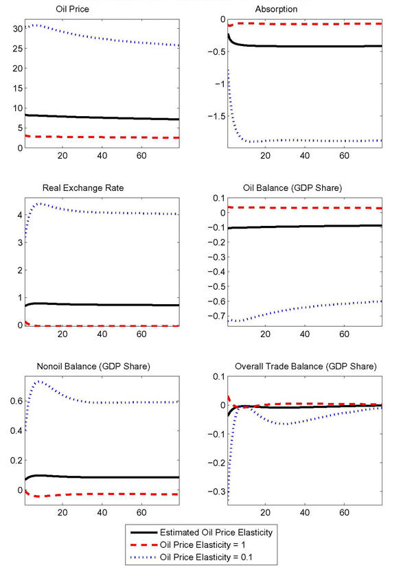
Figure 5: A Foreign Oil Supply Shock (Home Response) Alternative Oil Endowments
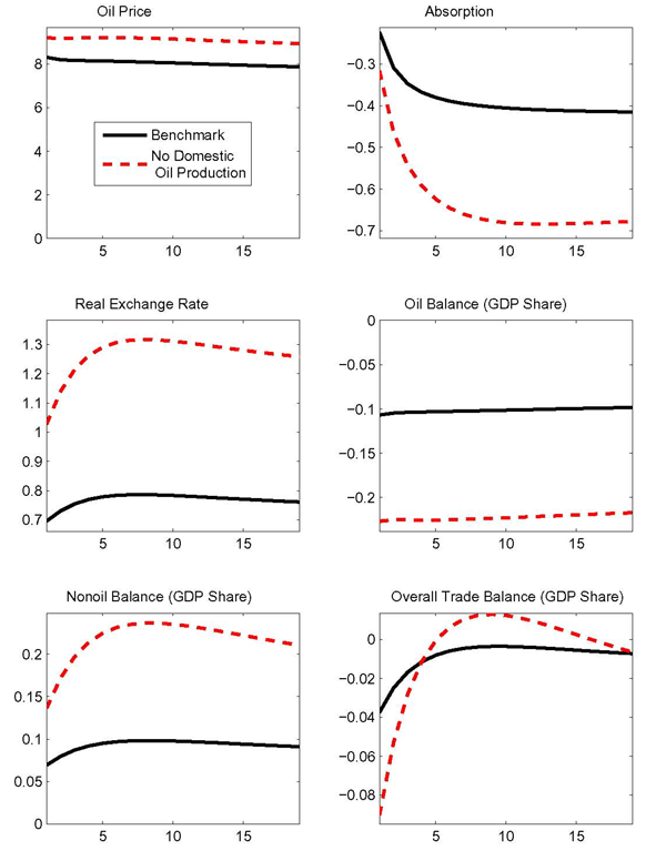
Figure 6: A Foreign Oil Supply Shock (Home Response) Alternative Financial Market Arrangements
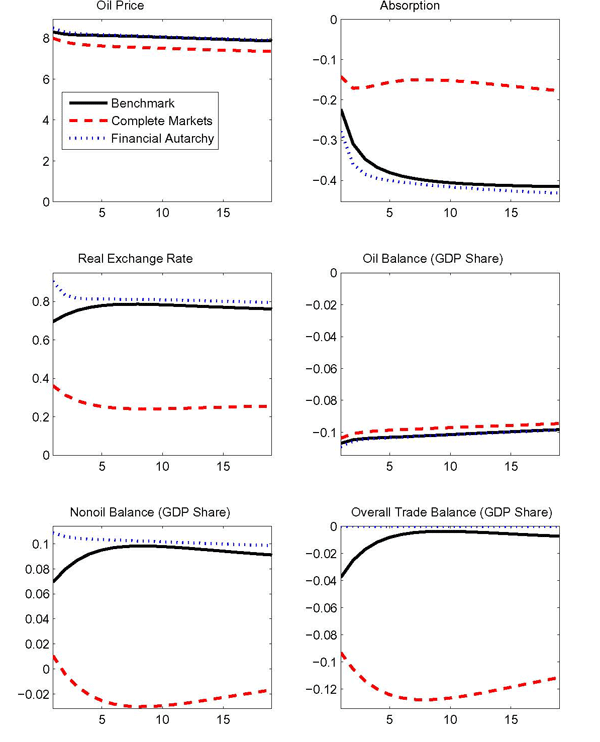
Figure 7: Hicks Decomposition of Home and Foreign Consumption Resopnse to a 20% Rise in the Oil Price
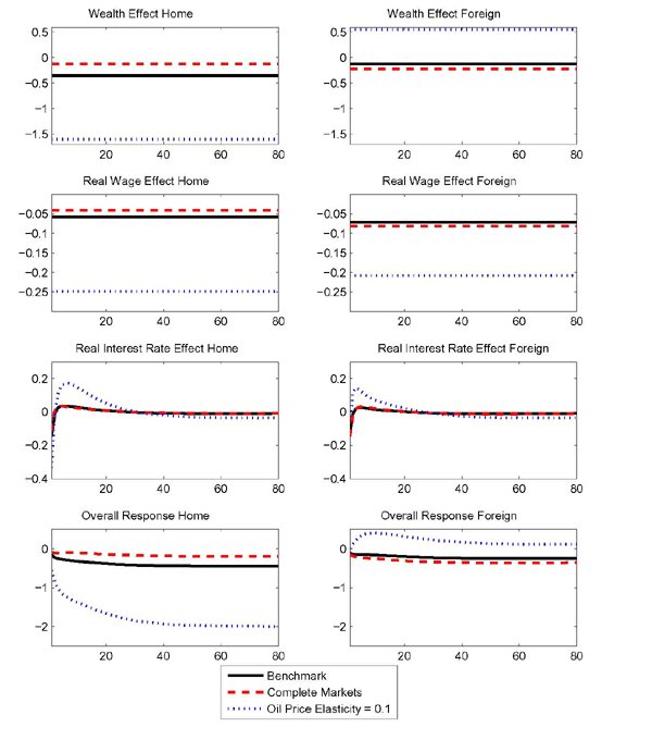
Figure 8: Hicks Decomposition of Home and Foreign Labor Resopnse to a 20% Rise in the Oil Price
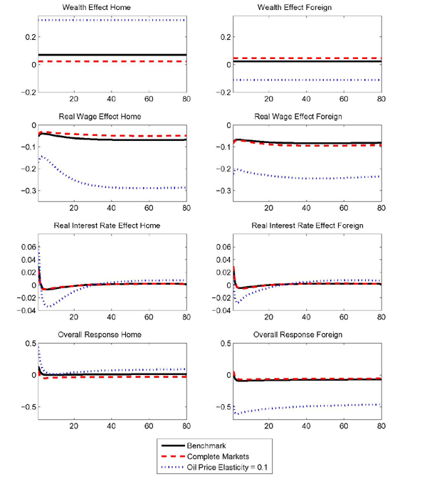
Figure 9: Technology and Oil Demand Shocks (Home Response) Technology and Oil Demand Shocks
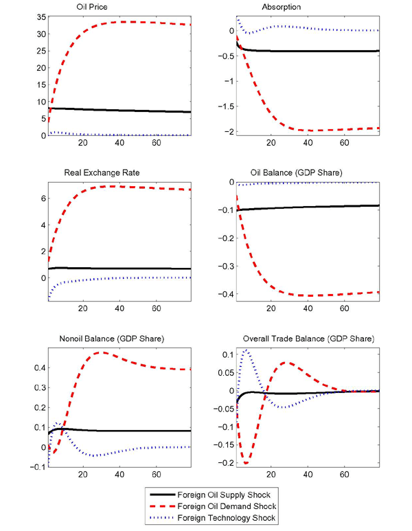
Footnotes
** The authors thank Christopher Gust, Lutz Kilian, Andrea Raffo, Luca Dedola and Eric Swanson for many insightful comments. We are particularly grateful to Giancarlo Corsetti (the editor) and two anonymous referees whose suggestions have greatly improved this paper. The views expressed in this paper are solely the responsibility of the authors and should not be interpreted as reflecting the views of the Board of Governors of the Federal Reserve System or of any other person associated with the Federal Reserve System. Return to text
*** Corresponding author. Telephone (202) 452 2550. E-mail [email protected]. Return to text
1. Kilian, Rebucci, and Spatafora (2009) used the identified VAR approach of [Kilian 2009] to estimate fundamental oil demand, supply, and activity shocks and uncover the response of several measures of the external balance for oil importers and exporters by regressing them on the identified shocks. Return to text
2. By "medium-run frequencies" we mean oscillations of amplitude between 6 and 200 quarters as suggested by Comin and Gertler (2006). Filtering the data at business cycle frequencies, typically 6 to 32 quarters, would exclude near permanent movements or slow-moving adjustments that are important ingredients in understanding fluctuations in the trade balance. Return to text
3. While Backus and Crucini (1998) had a similar focus on the consistent treatment of oil inputs in production in an international setting, the model dampened the importance of country specific wealth effects through the assumption of complete markets. Return to text
4. For instance, Baxter and Crucini (1995) showed that, for technology shocks, the equilibrium allocations in models where agents trade only one non state-contingent international bond are very close to those derived in an economy with complete international financial markets, provided that the technology shock is not permanent. Return to text
5. Jones, Leiby, and Paik ( 2004) offers a helpful overview of this literature. In our review we add more recent contributions and place greater emphasis on papers that model the international nature of the oil trade. Return to text
6. Hamilton (1983) used Granger causality tests and historical details of the oil industry to argue that exogenous price hikes preceded every U.S. postwar recession. [Mork 1989] found it important to distinguish between increases and decreases in oil prices. [Hamilton 2003] focused on the relative magnitude of increases. Return to text
7. Kilian, Rebucci, and Spatafora ( 2009) extended the analysis in [Kilian 2009] to encompass the reaction of open economy variables to oil shocks, also differentiating between oil importers and exporters. Return to text
8. A related study, Bruno and Sachs (1982b) also set up a macro econometric model in the style of the MPS but with a focus on the United Kingdom and found a long-run slowdown in productivity as a result of autonomous increases in commodity prices. Return to text
9. Rotemberg and Woodford (1996) extended the model of Kim and Loungani (1992) to allow for imperfect competition and found that departures from competitive behavior in the product market can amplify the effect of oil price fluctuations. Finn (2000) argued that such departures from perfect competition are not a necessary ingredient to generate substantial aggregate output effects from oil price increases. Instead, she introduced variable capacity utilization and assumed that capital utilization requires energy. Return to text
10. A separate strand of the closed economy literature has focused on putty-clay models in which the choice of capital is linked with a specific energy intensity at installation. See Atkeson and Kehoe (1999) and Wei (2003). Return to text
11. Earlier contributions on the Dutch disease that developed a static framework include: Bruno (1982), Corden and Neary (1982), Forsyth and Kay (1980), Neary and Purvis (1983). Further references can be obtained from the overview article by Corden (1984). Return to text
12. While Backus and Crucini (1998) had a similar focus on the consistent treatment of oil inputs in production in an international setting, their model dampened the importance of country specific wealth effects through the assumption of complete markets. We assume that financial markets are incomplete. Return to text
13. As discussed in Erceg, Guerrieri, and Gust ( 2006), our trade specification implies that the activity variable driving (nonoil) import and export demand can be regarded as a weighted average of consumption and investment, with the latter receiving a large weight consistent with the high weight of investment goods in U.S. trade. The paper also provides empirical support in favor of this specification over a specification in which the real activity variable driving trade is total absorption. See also Engel and Wang (2008). Return to text
14. A linear framework might appear at odds with the empirical work that has stressed asymmetries in the propagation of oil shocks to the macroeconomy. However, more recently, Kilian and Vigfusson (2009) found very little, if any, evidence of asymmetries in the response of U.S. GDP, unemployment, and gasoline consumption to energy price shocks. Return to text
15. The steady state around which we linearize depends on the relative level of technology in each country, which we initialize to unity. We evaluated the robustness of our solution procedure by using a nonlinear Newton-Raphson algorithm that does not rely on linearization around an initial steady state, and found that the results were nearly identical to those reported. Return to text
16. Absent this constraint, a shock to oil efficiency in production would be mostly offset by an adjustment of the oil use in consumption. Return to text
17. We fixed the error correction term at an arbitrary small value. When we allowed for AR(2) processes for technology, import preference shocks, and oil supply shock, the growth component was rejected by the data in each case. Return to text
18. We use the implementation of the bandpass filter derived by Christiano and Fitzgerald (2003). Return to text
19. We use quarterly data from 1974 through 2008. Series for U.S. GDP, oil imports, nonoil goods imports, and the overall goods trade balance are from the U.S. National Income and Products Accounts (NIPA). Series for U.S. and foreign oil production are from the Energy Information Administration of the U.S. Department of Energy. The relative price of oil is the ratio of the refiners' acquisition cost for imported crude obtained from the Energy Information Administration and the GDP deflator from NIPA. The series for foreign GDP is an export-weighted average of the GDP of the 26 most important trading partners of the United States. A description of the export weights can be found in Loretan (2005). The countries included account for well over 90% of U.S. exports as well as imports. Return to text
20. For instance Cooper (2003) estimated the long-run price elasticity of the demand for crude oil to be 0.45. Return to text
21. For instance, Hooper, Johnson, and Marquez ( 2000) estimated trade price elasticities using aggregate data for G-7 countries. They reported a long-run export price elasticity of 1.5 for the United States. Return to text
22. The benchmark calibration of the trade elasticity around unity implies an appreciation of the real exchange rate in reaction to a persistent contraction in technology. Return to text
23. These results on the importance of the energy intensity are in line with the empirical work of Davis and Haltiwanger (2001). Focusing on industry level data, instead of country differences, they emphasized that the magnitude of the employment response to oil shocks varies systematically with observable sectoral characteristics, rising with the oil intensity of the industry. Return to text
24. Local oil endowments differentiate our model further from that of Backus and Crucini (1998). In their framework such a distinction would play no role because of complete financial markets. Return to text
25. As described above, our benchmark calibration reflects cross-country differences in oil endowments and intensities. The nonoil balance and the real exchange rate would show no movement under complete markets, if oil endowments and intensities were chosen to be identical in the two countries (implying no oil trade in steady state). If the oil intensities in production and consumption were chosen to be identical across countries, but the endowments differed, the response of the real exchange rate would still be muted. Under incomplete markets, however, the nonoil balance would still have to improve even with no oil trade in steady state. Return to text
26. In our model, there is little distinction between the real exchange rate and the terms of trade. Return to text
27. However, for technology shocks the three financial market arrangements imply very similar allocations, as the trade elasticity is parameterized close to unity and the real exchange rate provides substantial insurance against technology shocks in our model. Return to text
28. The absence of a wealth effect in the foreign country does not imply, that consumption and labor are unaffected by the oil shock. However, these variables are impacted through the substitution effects caused by a lower real wage and a higher real interest rate. Return to text
29. The wage substitution effect on consumption is constant since our utility function is additive separable in consumption and leisure, and time separable. Return to text
30. The parametrization of the shock processes is determined by the moment matching exercise discussed in Section 4.1 and reported in Table 2. Return to text
31. Foreign consumption preference shocks, or foreign government spending shocks would also influence the price of oil in the model. However, as with technology shocks, the external adjustment mechanism would be dominated by the direct effects of those shocks, rather than oil market considerations. Return to text
This version is optimized for use by screen readers. Descriptions for all mathematical expressions are provided in LaTex format. A printable pdf version is available. Return to text