Skip to: [Printable Version (PDF)]

Board of Governors of the Federal Reserve System
International Finance Discussion Papers
Number 898, June 2007 --- Screen Reader Version*

Three Great American Disinflations

Michael Bordo, Christopher Erceg*, Andrew Levin, and Ryan Michaels

NOTE: International Finance Discussion Papers are preliminary materials circulated to stimulate discussion and critical comment. References in publications to International Finance Discussion Papers (other than an acknowledgment that the writer has had access to unpublished material) should be cleared with the author or authors. Recent IFDPs are available on the Web at http://www.federalreserve.gov/pubs/ifdp/. This paper can be downloaded without charge from the Social Science Research Network electronic library at http://www.ssrn.com/.

Abstract:

This paper analyzes the role of transparency and credibility in accounting for the widely divergent macroeconomic effects of three episodes of deliberate monetary contraction: the post-Civil War deflation, the post-WWI deflation, and the Volcker disinflation. Using a dynamic general equilibrium model in which private agents use optimal filtering to infer the central bank's nominal anchor, we demonstrate that the salient features of these three historical episodes can be explained by differences in the design and transparency of monetary policy, even without any time variation in economic structure or model parameters. For a policy regime with relatively high credibility, our analysis highlights the benefits of a gradualist approach (as in the 1870s) rather than a sudden change in policy (as in 1920-21). In contrast, for a policy institution with relatively low credibility (such as the Federal Reserve in late 1980), an aggressive policy stance can play an important signalling role by making the policy shift more evident to private agents.

Keywords: monetary policy regimes, transparency, credibility, sacrifice ratio.

JEL classification: E32, E42, E52, E58

Acknowledgements: We thank Gauti Eggertson, Benjamin Friedman, Dale Henderson, Jinill Kim, Lee Ohanian, Thomas Sargent, Anna Schwartz, Lars Svensson, John Taylor, Francois Velde, Marc Wiedenmeier, and Tack Yun for helpful comments and suggestions, as well as seminar participants at the annual American Economic Association Meeting in Chicago, Columbia University, the Federal Reserve Board, the Federal Reserve Bank of San Francisco, Harvard University, the fourth International Research Forum on Monetary Policy conference, and at an NBER workshop honoring Anna Schwartz. Bordo received financial support from the Federal Reserve Board on this project. The views expressed in this paper are solely the responsibility of the authors and should not be interpreted as reflecting the views of the Board of Governors of the Federal Reserve System or of any other person associated with the Federal Reserve System.

1  Introduction

Since at least the time of David Hume (1752) in the mid-18th century, it has been recognized that episodes of deflation or disinflation may have costly implications for the real economy, and much attention has been devoted to assessing how policy should be conducted to reduce such costs. The interest of prominent classical economists in these questions, including Hume, Thornton, and Ricardo, was spurred by practical policy debates about how to return to the gold standard following episodes of pronounced wartime inflation.¹Drawing on limited empirical evidence, these authors tried to identify factors that contributed to the real cost of deflation, including those factors controlled by policy. They advocated that a deflation should be implemented gradually, if at all; in a similar vein a century later, Keynes (1923) and Irving Fisher (1920) discussed the dangers of trying to quickly reverse the large runup in prices that occurred during World War I and its aftermath.

While the modern literature has provided substantial empirical evidence to support the case that deflations or disinflations are often quite costly , there is less agreement about the underlying factors that may have contributed to high real costs in some episodes, or that might explain pronounced differences in costs across episodes.² Indeed, disagreement about the factors principally responsible for influencing the costs of disinflation helped fuel contentious debates about the appropriate way to reduce inflation during the 1970s and early 1980s. Many policymakers and academics recommended a policy of gradualism-reflecting the view that the costs of disinflation were largely due to structural persistence in wage and price setting-while others recommended aggressive monetary tightening on the grounds that the credibility of monetary policy in the 1970s had sunk too low for gradualism to be a viable approach.

In this paper, we examine three notable episodes of deliberate monetary contraction: the post-Civil War deflation, the post-WWI deflation, and the Volcker disinflation. One goal of our paper is to use these episodes to illuminate the factors that influence the costs of monetary contractions. These episodes provide a fascinating laboratory for this analysis, insofar as they exhibit sharp differences in the policy actions undertaken, in the credibility and transparency of the policies, and in the ultimate effects on inflation and output. Our second objective is to evaluate the ability of a variant of the New Keynesian model that has performed well in fitting certain features of post-war U.S. data to account for these historical episodes.

Our paper begins by providing a historical overview of each of these episodes. In the decade following the Public Credit Act of 1869, which set a 10 year timetable for returning to the Gold standard, the price level declined gradually by 30 percent, while real output grew at a robust 4-5 percent per year. We argue that the highly transparent policy objective, the credible nature of the authorities' commitment, and gradual implementation of the policy helped minimize disruptive effects on the real economy. By contrast, while prices fell by a similar magnitude during the deflation that began in 1920, the price decline was very rapid, and accompanied by a sharp fall in real activity. We interpret the large output contraction as attributable to the Federal Reserve's abrupt departure from the expansionary policies that had prevailed until that time; fortunately, because the ultimate policy objective was clear (reducing prices enough to raise gold reserves), the downturn was fairly short-lived. Finally, the Volcker disinflation succeeded in reducing inflation from double digit rates in the late 1970s to a steady 4 percent by 1983, though at the cost of a severe and prolonged recession. We argue that the substantial costs of this episode on the real economy reflected the interplay both of nominal rigidities, and the lack of policy credibility following the unstable monetary environment of the previous 15 years.

We next attempt to measure policy predictability during each of the three episodes in order to quantify the extent to which each deflation was anticipated by economic agents. For the two earlier periods, we construct a proxy for price level forecast errors by using commodity futures data and realized spot prices. While these commodity price forecast errors provide very imperfect measures of errors in forecasting the general price level, we believe that they provide useful characterizations of the level of policy uncertainty during each period: in particular, the commodity price forecast errors in the early 1920s were much larger and more persistent than in the 1870s. This pattern confirms other evidence on policy predictability during each episode taken from bond yields, contemporary narrative accounts, and informal surveys. Finally, for the Volcker period, we utilize direct measures of survey expectations on inflation to construct inflation forecast errors, and show that forecast errors were large and extremely persistent, suggesting a high degree of uncertainty about the Federal Reserve's policy objectives.

We then examine whether a relatively standard DGSE model is capable of accounting for these different episodes. The model that we employ is a slightly simplified version of the models used by Christiano, Eichenbaum, and Evans (2005) and Smets and Wouters (2003). Thus, our model incorporates staggered nominal wage and price contracts with random duration, as in Calvo (1983) and Yun (1996), and incorporates various real rigidities including investment adjustment costs and habit persistence in consumption. The structure of the model is identical across periods, aside from the characterization of monetary policy. In particular, we assume that the monetary authority targets the price level in the two earlier episodes, consistent with the authorities desire to reinstate or support the Gold standard; by contrast, we assume that the Federal Reserve followed a Taylor-style interest rate reaction function in the Volcker period, responding to the difference between inflation and its target value. Moreover, we assume that agents had imperfect information about the Federal Reserve's inflation target during the Volcker episode, and had to infer the underlying target through solving a signal extraction problem.

We find that our simple model performs remarkably well in accounting for each of the three episodes. Notably, the model is able to track the sharp but transient decline in output during the 1920s, as well as generate a substantial recession in response to the monetary tightening under Volcker. More generally, we interpret the overall success of our model in fitting these disparate episodes as reflecting favorably on the ability of the New Keynesian model - augmented with some of the dynamic complications suggested in the recent literature - to fit important business cycle facts. However, one important twist is our emphasis on the role of incomplete information in accounting for the range of outcomes.

Finally, we use counterfactual simulations of our model to evaluate the consequences of alternative strategies for implementing a new nominal target (i.e., either a lower price level, or a lower inflation rate). We find that under a highly transparent policy regime, a new nominal target can be achieved with minimal fallout on the real economy, provided the implementation occurs over a period of at least 3-4 years. In this vein, we use model simulations to show that a more predictable policy of gradual deflation - as occurred in the 1870s - could have helped avoid the sharp post-WWI downturn. However, our analysis of the Volcker period emphasizes that the strong argument for gradualism under a transparent and credible monetary regime becomes less persuasive if the monetary regime lacks credibility. In this lower credibility case, an aggressive policy stance can play an important signalling role insofar as it makes a policy shift - such as a reduction in the inflation target - more apparent to private agents. Because inflation expectations adjust more rapidly than under a gradualist policy stance, output can rebound more quickly.

The rest of the paper proceeds as follows. Section 2 describes the three episodes, while Section 3 examines empirical evidence on the evolution of expectations during each episode. Section 4 outlines the model, and Section 5 describes the calibration. Section 6 matches the model to the salient features of the three episodes, and considers counterfactual policy experiments. Section 8 concludes.

2  Historical Background

2.1  The Post-Civil War Episode

Given the high cost of financing the Civil War, the U.S. government suspended gold convertibility in 1862 and issued fiat money ("greenbacks"). The monetary base expanded dramatically in the subsequent two years, precipitating a sharp decline in the value of greenbacks relative to gold. The dollar price of a standard ounce of gold rose from its official price of $20.67 that had prevailed since 1834 to over $40 by 1864 (the lower panel of Figure 1 shows an index of the greenback price of gold relative to its official price of $20.67). Despite some retracing in the late stages of the war, the dollar price of gold remained about 50 percent above its official price by the cessation of hostilities in mid-1865.

Following the war, there was widespread support for reverting to a specie standard at the pre-war parity. In the parlance of the period, this meant eliminating the "gold premium," the difference between the market price of gold and the official price. Using simple quantity theory reasoning, policymakers regarded monetary tightening as the appropriate instrument for achieving this objective: if the overall price level fell sufficiently, the dollar price of gold would drop, and the gold premium eventually disappear. Accordingly, Congress passed the Contraction Act in April 1866, with the backing of President Johnson. This act instructed the U.S. Treasury - the effective monetary authority during that period - to retire the supply of greenbacks. Given initial public support for a quick return to convertibility, the Treasury proceeded aggressively, reducing the monetary base about 20 percent between 1865 and 1867. However, the sharp price deflation that ensued had a contractionary impact on the economy, with certain sectors experiencing disproportionate effects (e.g., heavily leveraged farmers). Thus, Congress and President Johnson were forced to temporarily suspend monetary tightening in the face of strong public protest (Friedman and Schwartz, 1963).

President Grant promised to renew the march toward resumption when he delivered his first inaugural in March 1869, but with the important difference that the deflation would be gradual. The president received key legislative support with the passage of the Public Credit Act of 1869, which pledged that the Federal Government would repay its debt in specie within ten years. The long timeframe reflected the new political imperative of a gradualist approach. With further monetary contraction deemed infeasible, supporters of resumption planned to keep the money stock roughly constant, and allow prices to fall slowly as the economy expanded. This philosophy helped guide legislation, and in turn the U.S. Treasury's operational procedures for conducting monetary policy. Thus, Treasury policy kept the monetary base fairly constant through most of the 1870s, offsetting the issuance of National Bank notes with the retirement of Greenbacks. The Treasury's ability to adhere to this policy was facilitated by the passage of the Resumption Act in 1875, which sealed January 1, 1879 as the date of resumption of convertibility, and by the election of the hard-money Republican candidate Rutherford Hayes in the 1876 election.

As seen in the upper-left panel of Figure 1, these policies succeeded in producing a fairly smooth and continuous decline in the aggregate price level, and allowed the authorities to comfortably meet the January 1879 deadline for the resumption of specie payments. Furthermore, as shown in the upper-right panel, all three of the available measures of real output grew at a fairly rapid and steady pace over the period from 1869 to 1872. Of course, the worldwide financial panic of 1873 had marked consequences for U.S. markets and economic activity; nevertheless, real output growth over the decade of the 1870s was remarkably strong, averaging about 4 to 5 percent per year.³

This strong economic growth in the face of persistent deflation seems to have been made possible because of the slow and fairly predictable nature of the price decline between the passage of the Public Credit Act in 1869 and resumption a decade later. Two factors played an important role in making the price decline predictable. First, the ultimate objective of restoring the gold price to its official (pre-war) level was highly credible. This served to anchor expectations about the long-run expected price level within a fairly narrow range, so that uncertainty about the future price level mainly reflected uncertainty about the path of the real value of gold (in terms of goods). Second, it was clear after 1868 that the target of restoring convertibility would be achieved gradually. As discussed above, there was little support in Congress for returning to the rapid pace of monetary contraction that followed the Civil War.

Our contention that the policy of restoring gold convertibility at the official pre-war price was highly credible may seem difficult to reconcile with the political agitation in favor of Greenbacks that seemed a salient feature of the 1870s. But support for the Gold standard - both within the U.S. government, and the public at large - remained extremely strong in the post-Civil War period, so that the net effect of the political agitation was simply to graduate progress towards convertibility.⁴ This support for resumption stemmed in part from historical precedent: the United States had been on a specie standard for almost its entire history, dating to the passage of the Coinage Act of 1792. It also reflected deeply-seated views about how a specie standard protected private property rights against unjust seizure, which was regarded as a moral and political imperative.

Overall, this analysis suggests that it is appropriate to characterize the U.S. deflation experience over at least the 1869-79 period as one in which both the final objective of policy was transparent and credible, and which implied a fairly clear path for the overall price level. Moreover, the authorities appeared to place a large weight on minimizing the adverse consequences to the real economy, and hence were content to achieve convertibility gradually in an environment of predictable deflation.⁵

2.2  The Post-WWI Episode

The U.S. government suspended the gold standard de facto shortly after it entered World War I and began an enormous arms build-up that fueled inflation. President Wilson ordered the suspension and placed an embargo on the export of gold in order to protect the country's stock. In the absence of the embargo, high inflation likely would have triggered large outflows of gold: GNP prices rose almost 40 percent while the U.S. was at war, which was equal to the cumulative increase in prices over the previous 15-year period. Wartime inflation had its roots in a roughly twenty-fold increase in federal government expenditure from the time the U.S. entered the war in April 1917 to the armistice in November 1918 (see Firestone, 1960, Table A3).⁶

When the war ended, the embargo was lifted, and the Treasury and the Federal Reserve had to negotiate monetary policy in order to protect the Gold standard.⁷The Federal Reserve's Board of Governors included five appointees and two ex-officio members, the Secretary of Treasury and the Comptroller of the Currency. This governance structure gave the Secretary of the Treasury a disproportionate influence over monetary policy, since the five appointees to the Board were reluctant to cross the Treasury. Faced with a 25-fold increase in gross public debt after the War (Meltzer 2003), the Secretary refused to support an increase in discount rates despite an acceleration in inflation into double digits in 1919.⁸However, the Treasury's reputation was strongly linked to the success of the gold standard. In particular, U.S. law required the Federal Reserve to ensure a stock of monetary gold equal to at least 40 percent of the supply of base money. By November 1919, sizeable gold outflows put the legal minimum in sight, and the Treasury finally supported Board action to raise the discount rate.

Once freed to act, the Board raised the System-wide average discount rate over 2 percentage points between late 1919 and mid-1920 (see Figure 2). Although an eventual tightening of policy was anticipated insofar as private agents believed that the government was committed to defending the Gold standard, both the timing and severity of the contraction were a surprise. The highly persistent rise in nominal rates in the face of rapidly shifting expectations about inflation (i.e., towards deflation) represented a much tighter policy stance than agents had anticipated. As seen in Figure 2, the aggregate price level plunged 20 percent between mid-1920 and mid-1921, and commodity prices declined much more precipitously. Output also declined very abruptly, especially in manufacturing. As seen in Figure 2, the FRB's index of industrial production fell more than 30 percent between mid-1920 and early 1921, while manufacturing employment showed a commensurate decline. But the short-lived nature of the depression appears equally striking, as a robust expansion pushed output back to its pre-deflation level by early 1922.

The deflation of 1920 was recognized both by contemporary observers and by later historians as a dramatic event in U.S. monetary history. Irving Fisher (1934) was strongly critical of the Federal Reserve's role in engineering a "disastrous deflation" for which "millions of workers were thrown out of work." Friedman and Schwartz (1963) observed that the price decline was "perhaps the sharpest in the entire history of the United States" and characterized the output contraction as "one of the severest on record."

The industrial production and employment measures shown in Figure 2 indicate a much more severe recession than would be suggested from annual data for the aggregate economy.⁹ First, the magnitude of the downturn is obscured by its relatively transitory nature, particularly since the decline in output and employment began in mid-1920 and ended partway through the following year; indeed, Friedman and Schwartz argued that this recession was so abrupt that ``annual data provide a misleading indicator of its severity." Second, the fluctuations in real GNP were dampened by the stability of real agricultural output (which comprised a substantial fraction of aggregate output) and hence this measure is somewhat less relevant for gauging the effects of monetary policy during this period.¹⁰

As in the post-Civil War episode, the authorities' commitment to supporting the Gold Standard after WWI seems beyond doubt. By the 1920s, the Gold standard was entrenched as both a national and international norm, and even countries that had experienced much larger wartime inflations expected to return to gold. The high credibility of the monetary regime ultimately served an important role in allowing the economy to recover quickly once it was clear that prices had fallen enough. But clearly, the major difference between the episodes was in the Federal Reserve's decision to implement a very rapid deflation in the early 1920s, which contrasted starkly with the gradualist policy of 1869-1879. Influential Federal Reserve policymakers including Benjamin Strong believed that it was of foremost importance to reverse quickly most of the price level increase that had occurred since the U.S. entry into the war; while they acknowledged this might cause a substantial output contraction, they believed the recessionary effects would be transient and did not warrant dragging out the deflation (Meltzer 2003). Thus, policymakers kept nominal interest rates at elevated levels even as prices fell dramatically. This departure from traditional gold standard rules - which would have prescribed cutting interest rates in the face of a massive deflation and sizeable gold inflows - helped create a depression in activity through its effect on real interest rates.

2.3  The Volcker Disinflation

As of 1979, the Federal Reserve had been in operational control of U.S. monetary policy for about 25 years, even if it remained sensitive to the political climate. The Accord of 1951 between the central bank and the Treasury had ceded monetary policy to the Federal Reserve. For a dozen years after the Accord, the Federal Reserve generally maintained a low and steady inflation rate. But beginning in the mid-1960s, the Federal Reserve permitted inflation to rise to progressively higher levels. By the time President Carter appointed in 1979 a well-known inflation "hawk", Paul Volcker, to run the Federal Reserve, (GNP) price inflation had reached 9 percent.

Two months after taking office in August 1979, Volcker announced a major shift in policy aimed at rapidly lowering the inflation rate. Volcker desired the policy change to be interpreted as a decisive break from past policies that had allowed the inflation rate to rise to double digit levels (Figure 3). The announcement was followed by a series of sizeable hikes in the federal funds rate: the roughly 7 percentage point rise in the nominal federal funds rate between October 1979 and April 1980 represented the largest increase over a sixth month period in the history of the Federal Reserve System. However, this tight monetary stance was temporarily abandoned in mid-1980 as economic activity decelerated sharply. Reluctantly, the FOMC imposed credit controls and let the funds rate decline - moves that the Carter Administration had publically supported. The FOMC's policy reversal and acquiesence to political pressure was widely viewed as a signal that it was not committed to achieving a sustained fall in inflation (Blanchard, 1984). Having failed to convince price and wage setters that inflation was going to fall, GNP prices rose almost 10 percent in 1980.

The Federal Reserve embarked on a new round of monetary tightening in late 1980. The federal funds rate rose to 20 percent in late December, implying an ex post real interest rate of about 10 percent. Real ex post rates were allowed to fall only slightly from this extraordinarily high level over the following two years. Newly-elected President Reagan's support of Volcker's policy was significant in giving the Federal Reserve the political mandate it needed to keep interest rates elevated for a prolonged period, and provided some shield from growing opposition in Congress; cf. Feldstein (1993). This second and more durable round of tightening succeeded in reducing the inflation rate from about 10 percent in early 1981 to about 4 percent in 1983, but at the cost of a sharp and very prolonged recession. The OECD's measure of the output gap expanded by 6 percent between mid-1980 and mid-1982, and the unemployment rate (not shown) hovered at 10 percent until mid-1983.

While policymakers in the Gold standard environment examined in the earlier episodes had the advantage of a transparent and credible long-run nominal anchor, the Volcker disinflation was conducted in a setting in which there was a high degree of uncertainty about whether policymakers had the desire and ability to maintain low inflation rates. But notwithstanding that Federal Reserve policy during the 1970s and early 1980s merits some criticism for a lack of transparent objectives, it seems unlikely that simple announcements about long-run policy goals (e.g., an inflation target of three percent) would have carried much weight given the poor track record of the preceding two decades. Thus, it seems arguable that Volcker's FOMC had little hope of harnessing inflation expectations in a way that could facilitate lower inflation without sizeable output costs.

3  Policy Predictability: Empirical Evidence

Empirical evidence about the predictability of price decline that preceded Resumption in 1879 appears fairly limited. However, as argued by Friedman and Schwartz (1963) and later Calomiris (1985 and 1993), the behavior of longer term bond yields seems at least consistent with the view that private agents expected the dollar to appreciate (and prices to fall) by enough to support an eventual return to gold. As seen in Figure 4, the nominal yields on high quality greenback-denominated railroad bonds were actually somewhat lower than the yield on gold-denominated U.S. treasury bonds at the passage of the Public Credit Act in 1869. By that time, confidence was very high that the government would satisfy its obligation to repay its bonds in gold. Thus, drawing on uncovered interest parity, Friedman and Schwartz interpreted the lower interest rate on privately issued railroad bonds as suggesting that private agents on balance expected some appreciation of the greenback relative to gold. Of course, the simple difference between the interest rate series would understate expected appreciation of the Greenback to the extent that the interest rate on the railroad bonds included a premium for default risk.¹¹

Some evidence from commodity futures markets also appears consistent with our interpretation that the gradual price decline prior to Resumption was largely anticipated. Taking the futures price as a proxy for the expected price of a given commodity at a date K months ahead, we constructed a series of forecast errors as the difference between the realized commodity price and the (futures-based) forecast. The futures prices are on 4-5 month contracts (the longest maturities regularly available during that period) on pork, corn, wheat, and lard.¹² Given the paucity of observations on each individual commodity, Figure 1 pools forecast errors for all four of the commodities (yielding 30 observations over our 1871-78 sample period). The forecast errors seem relatively small, especially given the substantial volatility in spot prices of the underlying commodities: the average absolute error using these pooled observations is around 10 percent. Moreover, realized prices do not appear consistently lower than forecast (i.e., the forecast errors are not consistently negative). Despite obvious limitations of our data - including the short duration of futures contracts, and small number of observations - they are at least suggestive that agents were not surprised by declining prices.

There is considerably more evidence about the predictability of policy in the case of the deflationary episode following WWI. One very useful source is Harvard's Monthly Survey of General Business Conditions, which appeared as a monthly supplement to the Review of Economics and Statistics beginning in 1919. Harvard's Monthly Survey (HMS) interpreted recent financial and macroeconomic developments, and also made projections about the future evolution of output, prices, and short-term interest rates. While projections about individual macroeconomic series were primarily qualitative, the HMS did make some explicit forecasts about the likely duration of the business downturn during the course of 1920-21.

Drawing on the surveys from the first half of 1920, the HMS forecasters correctly predicted that the post-war inflation would be followed by a period of monetary retrenchment, and appeared to have a fairly clear understanding of the channels through which the monetary tightening would operate. In particular, they argued that the Federal Reserve's imposition of higher discount rates beginning in late 1919 would precipitate a fall in commodity prices, followed by a decline in consumer prices, wages, and business activity; but drawing on historical experience, they expected that lower prices would allow monetary easing, and promote a vigorous recovery within about a year.

The HMS forecasters turned out to be surprised by the severity of the monetary tightening, and by the associated magnitude of price and output decline. At the onset of the tightening, the HMS commented that "both the Treasury and the Federal Reserve Board have embarked on a policy of orderly deflation," and projected in April 1920 that "it does not seem probable ... that liquidation in the near future will cause prices to fall below the level of a year ago and perhaps not below the level of November 1918," suggesting an anticipated fall in commodity prices of only 15-20 percent.¹³ But in the wake of a 40 percent decline in commodity prices by early 1921 and depression in business activity, Bullock (1921) observed that he and the other HMS forecasters "had not expected a (monetary) reaction of such acute severity. We had looked for a return [of commodity prices] to some such level as had prevailed in the few months following the armistice, and as late as July expected nothing so drastic as the events of the last half of the year." Moreover, the HMS forecasters were forced to revise their optimistic initial predictions (made in the spring of 1920) that recovery would occur within a year as the sharp nature of the downturn became more apparent. The HMS attributed the severity of the downturn in part to persistently high interest rates, as interest rates remained elevated for a longer duration than in previous cyclical downturns dating back to the 1890s.¹⁴ Nevertheless, given the enormous price contraction by early 1921, the HMS forecasters were confident that prices would soon stabilize (as in fact occurred by late 1921), and that an eventual easing of monetary conditions would facilitate a rebound in real activity.

Commodity price forecast errors provide complementary evidence that prices fell more quickly and by a greater magnitude than expected by private agents. Figure 2 shows commodity price forecast errors for three individual commodities - corn, oats, and cotton - measured again as the realized price of each commodity minus the `` forecast" implied by the futures price.¹⁵In the post-World War I deflation, commodity price forecast errors turned consistently negative shortly after monetary policy was tightened in early 1920, and reached 50 percentage points or higher in absolute value terms. The average forecast errors over the 1920-21 tightening period are several times as large as the commodity price forecast errors derived from the post-Civil War data. But interestingly, forecast errors are generally much smaller after early 1921. This seems consistent with our intepretation that after a markedly lower price level was achieved, the policy environment became much more predictable, as agents expected the aggregate price level to remain roughly stable.

Lastly, we turn to the Volcker disinflation, for which there is considerable survey data available on inflation expectations at different horizons. Figure 3 plots the median projection of four quarter ahead GNP price inflation from the Survey of Professional Forecasters. The average inflation forecast error at a one year horizon (the gap between realized inflation over the subsequent year, the dash-dotted line, and the forecast, the dashed line) averaged about 2 percentage points over the 1981-84 period. Importantly, the inflation forecast errors show little tendency to die out, reflecting that inflation was consistently lower than what agents projected. The lower right panel of Figure 3 also contrasts the relatively quick decline in current inflation with the much more sluggish adjustment of long-run inflation expectations (as proxied by Barclay's projection of inflation 5-10 years ahead, and by the 10 year ahead inflation projection of the Philadephia Federal Reserve Bank). Taken together, the survey data suggests that inflation expectations were very slow to react to the decline in realized inflation, which we interpret as strong evidence that private agents doubted the ability or desire of policymakers to maintain low inflation rates. This interpretation is consistent with that of Goodfriend (1993) and Goodfriend and King (2005), who argued that the slow adjustment of inflation expectations was a primary factor accounting for the high nominal interest rates on long-term bonds that prevailed through most of the 1980s.

4  The Model

We utilize the same basic model to analyze each of the three historical episodes, aside from differences in the characterization of monetary policy. The model can be regarded as a slightly simplified version of the model utilized by Christiano, Eichenbaum and Evans (2005), and Smets and Wouters (2003). Thus, our model incorporates nominal rigidities by assuming that labor and product markets each exhibit monopolistic competition, and that wages and prices are determined by staggered nominal contracts of random duration (following Calvo (1983) and Yun (1996)). We also include various real rigidities emphasized in the recent literature, including habit persistence in consumption, and costs of changing the rate of investment. Given that our characterization of monetary policy differs across episodes, we defer this discussion to Section 6 (when we present simulation results for each episode).

4.1  Firms and Price Setting

Final Goods Production As in Chari, Kehoe, and McGratten (2000), we assume that there is a single final output good $Y_{t}$ that is produced using a continuum of differentiated intermediate goods $Y_{t}(f).$ The technology for transforming these intermediate goods into the final output good is constant returns to scale, and is of the Dixit-Stiglitz form:

$$Y_{t}=\left[ \int_{0}^{1}Y_{t}\left( f\right) ^{\frac{1}{1+\theta_{p}} }df\right] ^{1+\theta_{p}}$$ (1)

where $\theta_{p}>0$.

Firms that produce the final output good are perfectly competitive in both product and factor markets. Thus, final goods producers minimize the cost of producing a given quantity of the output index $Y_{t}$, taking as given the price $P_{t}\left( f\right)$ of each intermediate good $Y_{t}(f)$. Moreover, final goods producers sell units of the final output good at a price $P_{t}$ that is equal to the marginal cost of production:

$$P_{t}=\left[ \int_{0}^{1}P_{t}{}\left( f\right) ^{\frac{-1}{\theta_{p}} }df\right] ^{-\theta_{p}}$$ (2)

It is natural to interpret $P_{t}$ as the aggregate price index.

Intermediate Goods Production A continuum of intermediate goods $Y_{t}(f)$ for $f\in\lbrack0,1]$ is produced by monopolistically competitive firms, each of which produces a single differentiated good. Each intermediate goods producer faces a demand function for its output good that varies inversely with its output price $P_{t}\left( f\right) ,$ and directly with aggregate demand $Y_{t}:$

$$Y_{t}\left( f\right) =\left[ \frac{P_{t}\left( f\right) }{P_{t}}\right] ^{\frac{-\left( 1+\theta_{p}\right) }{\theta_{p}}}Y_{t}$$ (3)

Each intermediate goods producer utilizes capital services $K_{t}\left( f\right)$ and a labor index $L_{t}\left( f\right)$ (defined below) to produce its respective output good. The form of the production function is Cobb-Douglas:

$$Y_{t}\left( f\right) =K_{t}(f)^{\alpha}L_{t}(f)^{1-\alpha}$$ (4)

Firms face perfectly competitive factor markets for hiring capital and the labor index. Thus, each firm chooses $K_{t}\left( f\right)$ and $L_{t}\left( f\right)$, taking as given both the rental price of capital $R_{Kt}$ and the aggregate wage index $W_{t}$ (defined below). Firms can costlessly adjust either factor of production. Thus, the standard static first-order conditions for cost minimization imply that all firms have identical marginal cost per unit of output. By implication, aggregate marginal cost $MC_{t}$ can be expressed as a function of the wage index $W_{t}$, the aggregate labor index $L_{t}$, and the aggregate capital stock $K_{t}$, or equivalently, as the ratio of the wage index to the marginal product of labor $MPL_{t}$:

$$MC_{t}=\frac{W_{t}L_{t}^{\alpha}}{\left( 1-\alpha\right) K_{t}^{\alpha} }=\frac{W_{t}}{MPL_{t}}$$ (5)

We assume that the prices of the intermediate goods are determined by Calvo-Yun style staggered nominal contracts. In each period, each firm f faces a constant probability, $1-\xi_{p}$, of being able to reoptimize its price $P_{t}(f)$. The probability that any firm receives a signal to reset its price is assumed to be independent of the time that it last reset its price. If a firm is not allowed to optimize its price in a given period, we follow Yun (1996) by assuming that it simply adjusts its price by the steady state rate of inflation $\Pi$ (i.e., $P_{t}(f)=\pi P_{t-1}(f))$. Finally, the firm's output is subsidized at a fixed rate $\tau_{p}$ (this allows us to eliminate the monopolistic competition wedge in prices by setting $\tau_{p}=\theta_{p}$).

4.2  Households and Wage Setting

We assume a continuum of monopolistically competitive households (indexed on the unit interval), each of which supplies a differentiated labor service to the production sector; that is, goods-producing firms regard each household's labor services $N_{t}\left( h\right)$, $h\in\lbrack0,1]$, as an imperfect substitute for the labor services of other households. It is convenient to assume that a representative labor aggregator (or "employment agency") combines households' labor hours in the same proportions as firms would choose. Thus, the aggregator's demand for each household's labor is equal to the sum of firms' demands. The labor index $L_{t}$ has the Dixit-Stiglitz form:

$$L_{t}=\left[ \int_{0}^{1}N_{t}\left( h\right) ^{\frac{1}{1+\theta_{w}} }dh\right] ^{1+\theta_{w}}$$ (6)

where $\theta_{w}>0$. The aggregator minimizes the cost of producing a given amount of the aggregate labor index, taking each household's wage rate $W_{t}\left( h\right)$ as given, and then sells units of the labor index to the production sector at their unit cost $W_{t}$:

$$W_{t}=\left[ \int_{0}^{1}W_{t}{}\left( h\right) ^{\frac{-1}{\theta_{w}} }dh\right] ^{-\theta_{w}}$$ (7)

It is natural to interpret $W_{t}$ as the aggregate wage index. The aggregator's demand for the labor hours of household $h$ - or equivalently, the total demand for this household's labor by all goods-producing firms - is given by

$$N_{t}\left( h\right) =\left[ \frac{W_{t}\left( h\right) }{W_{t}}\right] ^{-\frac{1+\theta_{w}}{\theta_{w}}}L_{t}$$ (8)

The utility functional of a typical member of household $h$ is

$$\mathbb{E}_{t}\sum_{j=0}^{\infty}\beta^{j}\{\frac{1}{1-\sigma}\left( C_{t+j}\left( h\right) -\varkappa C_{t+j-1}(h)\right) ^{1-\sigma }+$$ (9)

$$\frac{\chi_{0}}{1-\chi}(1-N_{t+j}\left( h\right) )^{1-\chi}+\frac{\mu _{0}}{1-\mu}\left( \frac{M_{t+j}\left( h\right) }{P_{t+j}}\right) ^{1-\mu }\}$$ (10)

where the discount factor $\beta$ satisfies $0<\beta<1.$ The dependence of the period utility function on consumption in both the current and previous period allows for the possibility of external habit persistence in consumption spending (e.g., Smet and Wouters, 2003). In addition, the period utility function depends on current leisure $1-N_{t}\left( h\right)$, and current real money balances. $\frac{M_{t}\left( h\right) }{P_{t}}.$

Household $h$'s budget constraint in period $t$ states that its expenditure on goods and net purchases of financial assets must equal its disposable income:

$$\begin{array}[c]{c} P_{t}C_{t}\left( h\right) +P_{t}I_{t}\left( h\right) +\frac{1}{2}\psi _{I}P_{t}\frac{\left( I_{t}(h)-I_{t-1}(h)\right) ^{2}}{I_{t-1}(h)}\\ \\ M_{t+1}\left( h\right) -M_{t}\left( h\right) +\int_{s}\xi_{t,t+1} B_{D,t+1}(h)-B_{D,t}(h)\\ \\ =(1+\tau_{W})W_{t}\left( h\right) N_{t}\left( h\right) +R_{Kt} K_{t}(h)+\Gamma_{t}\left( h\right) -T_{t}(h)\\ \end{array}$$ (11)

Thus, the household purchases the final output good (at a price of $P_{t}),$ which it chooses either to consume $C_{t}\left( h\right)$ or invest $I_{t}\left( h\right)$ in physical capital. The total cost of investment to each household h is assumed to depend on how rapidly the household changes its rate of investment (as well as on the purchase price). Our specification of such investment adjustment costs as depending on the square of the change in the household's gross investment rate follows Christiano, Eichenbaum, and Evans (2005). Investment in physical capital augments the household's (end-of-period) capital stock $K_{t+1}(h)$ according to a linear transition law of the form:

$$K_{t+1}\left( h\right) =(1-\delta)K_{t}(h)+I_{t}(h)$$ (12)

In addition to accumulating physical capital, households may augment their financial assets through increasing their nominal money holdings ( $M_{t+1}\left( h\right) -M_{t}\left( h\right) ),$ and through the net acquisition of bonds. We assume that agents can engage in frictionless trading of a complete set of contingent claims. The term $\int_{s}\xi_{t,t+1} B_{D,t+1}(h)-B_{D,t}(h)$ represents net purchases of state-contingent domestic bonds, with $\xi_{t,t+1}$ denoting the state price, and $B_{D,t+1}\left( h\right)$ the quantity of such claims purchased at time $t$. Each member of household $h$ earns labor income $(1+\tau_{W})W_{t}\left( h\right) N_{t}\left( h\right)$ (where $\tau_{W}$ is a subsidy that allows us to offset monopolistic distortions in wage-setting) , and receives gross rental income of $R_{Kt}K_{t}(h)$ from renting its capital stock to firms. Each member also receives an aliquot share $\Gamma_{t}\left( h\right) \,$of the profits of all firms, and pays a lump-sum tax of $T_{t}\left( h\right)$ (this may be regarded as taxes net of any transfers).

In every period $t$, each member of household $h$ maximizes the utility functional (9) with respect to its consumption, investment, (end-of-period) capital stock, money balances, and holdings of contingent claims, subject to its labor demand function (8), budget constraint (11), and transition equation for capital (12). Households also set nominal wages in Calvo-style staggered contracts that are generally similar to the price contracts described above. Thus, the probability that a household receives a signal to reoptimize its wage contract in a given period is denoted by $1-\xi_{w}$, and as in the case of price contracts this probability is independent of the date at which the household last reset its wage. However, we specify a dynamic indexation scheme for the adjustment of the wages of those households that do not get a signal to reoptimize, i.e., $W_{t}(h)=\omega_{t}W_{t-1}(h),$in contrast to the static indexing assumed for prices. As discussed by Christiano, Eichenbaum, and Evans (2005), dynamic indexation of this form introduces some element of structural persistence into the wage-setting process. Our asymmetric treatment is motivated by the empirical analysis of Levin, Onatski, Williams, and Williams (2005). These authors estimated a similar model using U.S. data over the 1955:1-2001:4 period, and found evidence in favor of nearly full indexation of wages, but not of prices (hence our specification of prices as purely forward-looking).

4.3  Fiscal Policy and the Aggregate Resource Constraint

The government's budget is balanced every period, so that total lump-sum taxes plus seignorage revenue are equal to output and labor subsidies plus the cost of government purchases:

$$\begin{tabular}[c]{l} $M_{t}-M_{t-1}+\int_{0}^{1}T_{t}\left( h\right) dh=\int_{0}^{1}\tau_{p} P_{t}\left( f\right) Y_{t}\left( f\right) df+\int_{0}^{1}\tau_{w} W_{t}\left( h\right) N_{t}\left( h\right) dh+P_{t}G_{t}$ \end{tabular}$$ (13)

where $G_{t}$ indicates real government purchases. We assume that government spending is a fixed share of output in our analysis. Finally, the total output of the service sector is subject to the following resource constraint:

$$Y_{t}=C_{t}+I_{t}+G_{t}$$ (14)

5  Solution and Calibration

To analyze the behavior of the model, we log-linearize the model's equations around the non-stochastic steady state. Nominal variables, such as the contract price and wage, are rendered stationary by suitable transformations. We then compute the reduced-form solution of the model for a given set of parameters using the numerical algorithm of Anderson and Moore (1985), which provides an efficient implementation of the solution method proposed by Blanchard and Kahn (1980).

5.1  Parameters of Private Sector Behavioral Equations

The model is calibrated at a quarterly frequency. Thus, we assume that the discount factor $\beta=.9925,$ consistent with a steady-state annualized real interest rate $\overline{r}$ of about 3 percent. We assume that the subutility function over consumption is logarithmic, so that $\sigma=1,$ while we set the parameter determining the degree of habit persistence in consumption $\varkappa$ = 0.6 (similar to the empirical estimate of Smets and Wouters 2003). The parameter $\chi,$ which determines the curvature of the subutility function over leisure, is set equal to 10, implying a Frisch elasticity of labor supply of 1/5. This is considerably lower than if preferences were logarithmic in leisure, but within the range of most estimates from the empirical labor supply literature. The scaling parameter $\chi_{0}$ is set so that employment comprises one-third of the household's time endowment, while the parameter $\mu_{0}$ on the subutility function for real balances is set an arbitrarily low value (so that variation in real balances has a negligible impact on other variables). The share of government spending of total expenditure is set equal to 12 percent.

The capital share parameters $\alpha=1/3$. The quarterly depreciation rate of the capital stock $\delta=0.02$, implying an annual depreciation rate of 8 percent. The price and wage markup parameters $\theta_{P}=\theta_{W}=1/5$. We set the cost of adjusting investment parameter $\phi_{I}$ = 2, which is somewhat smaller than the value estimated by Christiano, Eichenbaum, and Evans (2001) using a limited information approach; however, the analysis of Erceg, Guerrieri, and Gust (2005) suggests that a lower value in the range of unity may be better able to capture the unconditional volatility of investment within a similar modeling framework. We assume that price contracts last three quarters, while nominal wage contracts last four quarters. The calibration of contract duration is in the range typically estimated in the literature.

6  Model Simulations

6.1  The Post Civil War Deflation

While we will attempt to use our model to account for the evolution of real activity during the latter two episodes - on the premise that monetary changes played a principal role in driving the output fluctuations that occurred - our objective in applying the model to the post Civil War deflation is narrower in scope. In particular, while a more complicated model with a richer set of shocks would be required to account for output behavior over the long period prior to Resumption, our focus here is simply to rationalize why the "secular" deflation of 2-3 percent per year appeared to exert little drag on output growth in the decade following the Public Credit Act of 1869.

In this vein, we characterize the monetary authorities in the 1869-1879 period as following a simple targeting rule derived from minimizing a loss function that depends on the gap between the price level $p_{t}$ and its target value $p_{t}^{\ast}$ (which we call the price level gap), and on the output gap $g_{t}$. Under a quadratic period loss function in each of these gaps, the targeting rule is derived by minimizing a discounted conditional loss function of the form:

$$\mathbb{E}_{t}\sum_{j=0}^{\infty}\beta^{j}\left\{ (p_{t+j}-p_{t+j}^{\ast })^{2}+\lambda_{G}g_{t+j}^{2}\right\}$$ (15)

subject to the behavioral constraints implied by household and firm optimization from the model of Section 4.¹⁶

The solid blue line in Figure 5 presents our benchmark characterization of the post Civil War deflation period in response to a permanent reduction in $p_{t}^{\ast}$ of 30 percent. The weight on the output gap in the loss function is chosen to stretch out the price decline over the course of a decade, so that the simulated price level decline appears quite similar to the historical experience (this is achieved by setting $\lambda_{G}=5000$ in (15)). It is evident from the figure that the large cumulative decline in prices has little impact on real activity: in fact, output never falls more than 0.1 percent below potential. The optimal policy achieves this sizeable price decline at minimal output cost by relying heavily on an "expectations channel": current price-setters are willing to lower prices today in the expectation that future prices will be lower (and hence deflation does not require a recession). A notable characteristic of the optimal policy is that it implies a persistent decline in short-term nominal interest rates, which is consistent with the policy shift exerting little effect on long-term real interest rates.

We believe that this simple characterization of policy captures many of the relevant features of the historical environment following the passage of the Public Credit Act in 1869 that were recounted in Section 2. These features included: first, the mandate to effect a substantial reduction in the general price level, subject to the proviso that the deflation would be gradual enough to avoid a reprise of the post war monetary recession; and second, the ability of the authorities to commit to such a policy. Admittedly, our characterization abstracts from some aspects of implementation that were discussed in Section 2, including the operational procedure of controlling the monetary base. However, taking account of such features would require significant complications to our model, and would seem highly unlikely to change our basic message that a very gradual and predictable deflation exerts small effects on real activity under a reasonable and well-understood rule (specified either in terms of the money stock or nominal interest rate).¹⁷

Given the negligible output losses under the ten year implementation window, it is also natural to inquire whether the 1869-1879 price level decline could have occurred more rapidly without significantly exacerbating the effects on the real economy: did the authorities perhaps become overly cautious in response to the public acrimony that followed their first attempts to deflate? This rather general question about how quickly a deflation can be implemented without causing substantial fallout on the real economy has close parallel in earlier work by Taylor (1983) and Ball (1994b, 1995), but with the important difference that the latter authors assessed how the real costs depended on the horizon over which the inflation rate was changed, rather than the price level. While these authors found that a disinflation could be implemented over a short horizon of roughly two years or less with minimal output costs, our results suggest that a considerably longer horizon is required to implement a change in the price level; the difference reflects that while the staggered contracts framework implies little endogenous persistence in the inflation rate - so that it is relatively easy for inflation to jump - it implies considerably more price level persistence. Under our baseline calibration, the implied tradeoff between a shorter horizon for implementing the disinflation and higher output losses can be derived by varying the relative weight on the output gap ( $\lambda_{G})$ in the targeting rule (15). Two alternative cases are shown in Figure 5. The dashed green line shows that a value of $\lambda_{G}$ which causes the 30 percent price decline to occur over only four years causes the output loss to rise to about 1 percent, which still seems quite modest. However, while our benchmark model allows an inflation target to be reduced over a narrow 2 year window with minimal output losses (as verified below, consistent with the earlier literature cited), implementing a new price level target over such an abbreviated time frame causes a pronounced recession (as depicted by the red dash-dotted line).

These results suggest that the ten-year window for phasing in the deflation might have been reduced considerably without much of an adverse effect on output. Moreover, to the extent that wages and prices may have been somewhat more flexible in this episode than implied by our benchmark calibration, the output losses associated with shortening the implementation horizon would be mitigated relative to those indicated in Figure 5. Nevertheless, provided there is some sluggishness in prices and wages - even if less than embedded in our benchmark - real interest rates must rise sharply to implement a discrete downward shift in the price level over a short horizon. Thus, it is arguable that a short implementation window in the neighborhood of a year or two might have risked a substantial recession.

6.2  The Post-WWI Deflation

We now turn to using our model to characterize the severe monetary recession that began in 1920. As discussed above, the salient feature was a precipitous and largely unexpected decline in the price level of about 20 percent over a period of less than two years, and a sharp but fairly short-lived contraction in activity. Our model simulations in Figure 5 suggest that attempting to achieve a new price level objective so quickly would precipitate a severe recession even under a well-designed policy derived in an optimization-based setting. But given that monetary policy seemed far from optimal during the 1920s, it remains of interest to assess the implications of a large shift in the price level target under an alternative monetary rule that may better account for the nature of policy.

Despite obvious difficulties in characterizing policy during this turbulent period, we believe that many of the prominent features of the policymaking framework can be summarized in a simple instrument rule of the form:

$$i_{t}=\gamma_{i}i_{t-1}+\gamma_{P}(p_{t}-p_{t}^{\ast})$$ (16)

This rule posits the nominal interest rate $i_{t}$ as responding to the price level gap $(p_{t}-p_{t}^{\ast})$, as well as to its own lag (a constant term is suppressed for simplicity). This specification has two salient features. First, policy rates are driven exclusively by the difference between the current price level and its target $p_{t}^{\ast}.$ This specification is intended to capture the belief of key Federal Reserve policymakers that continued adherence to the Gold standard hinged on rolling back the rise in the U.S. price level that had occurred following the U.S. entry into the war. While it was recognized that real activity might suffer in the short-run, it was regarded of paramount importance to reduce prices enough to faciliate an adequate buildup of gold reserves. The second key feature of (16) is that nominal rates do not respond to inflation (either ex post or ex ante). As shown below, this helps account for the empirical observation that nominal rates remained high despite an enormous decline in the price level in 1920-21. This feature of the instrument rule evidently contrasts with the behavior of nominal rates under the optimal rule shown in Figure 5, in which declining inflation exerts sizeable downward pressure on nominal rates.

The price level target is assumed to follow an exogenous random walk, so that any shift in the target is perceived as permanent. The shock we consider involves a 20 percent cumulative reduction in $p_{t}^{\ast}$ that begins in 1920q1. While private agents are assumed to observe the underlying price level target, we assume that the shock is phased-in over three quarters, in part to match the modest persistence suggested by the commodity price forecast errors discussed in Section 3. Finally, we set $\gamma_{i}=.5$ to allow for a bit of interest rate smoothing, and $\gamma_{P}=.12$ in order to allow our model to do reasonably well in matching the rise in nominal interest rates that occurred in the historical episode.

Simulation results for our benchmark case are shown by the solid blue lines in Figure 6. The model simulation generates a large decline in the price level beginning in 1920 that is similar in magnitude to that observed. The sharpness of this price decline is well-captured by our modelling framework, in which prices are determined by Calvo-style contracts with no dynamic indexation. The speed of the price decline would be much more difficult to rationalize in a model that incorporated dynamic indexation or other forms of intrinsic inflation persistence.

The model implies a pronounced output decline that is followed by a rapid recovery, which is similar to the pattern observed historically. The output decline in our model simulation is attributable to a sizeable and fairly persistent rise in the real interest rate. The substantial rise in real long-term interest rates despite little movement in the nominal interest rate reflects both that agents came to expect large price declines, and that policy would maintain high nominal rates even in a deflationary environment.¹⁸

Thus, our simulation results suggest that the high costs of the 1920-21 deflation reflect that the Federal Reserve attempted to engineer an extremely rapid deflation, and that it was perceived as following a monetary policy stance in which future nominal rates were expected to remain high (at least for a few quarters) in the face of deflation: in effect, consistent with our historical analysis, the Federal Reserve used the blunt instrument of a severe recession to push down prices, rather than operating through an expectations channel. Accordingly, it is of interest to consider the counterfactual simulation depicted by the dotted green lines, which shows a case in which the central bank is assumed to change its target path level incrementally, and to follow a rule in which the nominal interest rate also responds to ex post inflation (but is otherwise identical to equation (16)). Clearly, while allowing for nominal rates to decline with inflation would have induced a more gradual convergence in prices to target, it would have greatly ameliorated the output costs. Obviously, even more favorable outcomes could be derived to the extent that policy could better approximate the optimal targeting rules discussed in the previous section rather than a simple ad hoc instrument rule.

6.3  The Volcker Disinflation

A striking feature of the Volcker disinflation period was the fact that inflation forecast errors were extremely persistent. Erceg and Levin (2003) argued that the persistence in the forecast errors - and associated high persistence in realized inflation - may have reflected a high level of uncertainty about the central bank's inflation target.¹⁹In this paper, we take a similar stylized approach to characterizing uncertainty about the inflation target of the central bank by assuming that agents cannot differentiate permanent shocks to the inflation target from transient shocks to the monetary policy reaction function.

We specify the central bank's reaction function over the Volcker period as a slightly modified version of the Taylor rule:

$$i_{t} = \gamma_{i} i_{t-1} + (1-\gamma_{i})(\bar{r} + \pi_{t}) + \gamma_{\pi} (\pi_{t} - \pi^{\ast}_{t}) + \gamma_{y} (\Delta y_{t} - \bar{g}) + e_{t}$$ (17)

where $i_{t}$ is the short-term nominal interest rate, $\pi_{t}$ is the four-quarter change in the GDP price deflator, $\pi_{t}^{\ast}$ is the central bank's inflation target, $\Delta y_{t}$ is the four-quarter change in real GDP, and $e_{t}$ denotes the shock to the policy reaction function, where all variables are expressed at annual rates in percentage points.²⁰

In estimating this policy reaction function, we utilize the sample period 1980:4 through 1986:4, thereby excluding the policy reversals that occurred during the first year of Volcker's tenure (as discussed in section 2.3).²¹ Least squares estimation over this sample period yields $\gamma_{i}=0.65,$ $\gamma_{\pi}=0.59,$ and $\gamma_{y}=0.30.$ As seen in Figure 7, this simple form of the reaction function accounts reasonably well for the evolution of the funds rate over the sample period.

Agents cannot directly observe the long-run inflation target $\pi_{t}^{\ast},$ or the monetary shock $e_{qt};$ but given that agents observe interest rates, inflation, and output growth (as well as all of the structural parameters of the model), they can infer a composite shock $\phi_{t}$ which is a hybrid of the inflation target shock and the monetary policy shock:

$$\phi_{t}=-\gamma_{G}\pi_{t}^{\ast}+e_{t}$$ (18)

The unobserved components in turn are perceived to follow a first-order vector autoregression:

$$\begin{array}[c]{c} \left[ \begin{array}[c]{c} \pi_{t}^{\ast}\\ e_{t} \end{array} \right] =\left[ \begin{array}[c]{cc} \rho_{p} & 0\\ 0 & \rho_{q} \end{array} \right] \left[ \begin{array}[c]{c} \pi_{t-1}^{\ast}\\ e_{t-1} \end{array} \right] +\left[ \begin{array}[c]{cc} \upsilon_{1} & 0\\ 0 & \upsilon_{2} \end{array} \right] \left[ \begin{array}[c]{c} \varepsilon_{pt}\\ \varepsilon_{qt} \end{array} \right] \\ \end{array}$$ (19)

The inflation target $\pi_{t}^{\ast}$ is highly persistent, and has an autoregressive root $\rho_{p}$ arbitrarily close to unity. For simplicity, we assume that the random policy shock $e_{t}$ is white noise (so $\rho_{q}=0)$. The innovations associated with each shock, $\varepsilon_{pt}$ and $\varepsilon_{qt}$, are mutually uncorrelated with unit variance.

Given this linear structure, we assume that agents use the Kalman filter to make optimal projections about the unobserved inflation target $\pi_{t}^{\ast}.$ The inflation target perceived by agents evolves according to a first order autoregression. Agents update their assessment of the inflation target by the product of the forecast error innovation and a constant coefficient. This coefficient, which is proportional to the Kalman gain, can be expressed as a function of the signal-to-noise ratio $(\gamma_{\pi}\frac{v_{1}}{v_{2}}).$ Clearly, the signal-to-noise ratio depends on the relative magnitude of innovations to each of the components of the observed shock $\phi_{t};$ but importantly, it also depends directly on the weight $\gamma_{\pi}$ on the inflation target in the central bank's reaction function. Intuitively, if policy is aggressive in reacting to the inflation gap, agents will attribute more of any unexplained rise in interest rates to a reduction in the central bank's long-run inflation target, rather than to random policy shocks.

As argued by Erceg and Levin (2003) in the context of a somewhat simpler dynamic model, the signal-to-noise ratio plays a crucial role in affecting model responses to a shock to the inflation target. Following their approach, we estimate this composite parameter (i.e., $\frac{v_{1}}{v_{2}},$ using the estimated value of $\gamma_{\pi})$ by choosing the value that minimizes the difference between historical four-quarter-ahead expected inflation (taken from survey data) and the corresponding expected inflation path implied by our model.²²) In particular, we minimize the loss function:

$$Loss \sum_{j=0}^{20}\left[ \mathbb{E}_{t+j}(\pi_{t+3+j} ^{4}(survey\text{ }data\text{)-}\mathbb{E}_{t+j}(\pi_{t+3+j}^{4} (\operatorname{mod}el\text{)}\right] ^{2}$$ (20)

The estimation period is 1980:4 through 1985:4. The model expectation in (20) is the expected rate of four-quarter ahead inflation that agents project at each date, given an assumed one-time shift in the inflation target of six percentage points that occurs in 1980:4. Our estimation routine yields a point estimate of $(\frac{v_{2}}{v_{1}})$ that implies a Kalman gain coefficient on the forecast error innovation of about 0.10.

Figure 8 shows the effects of a six percentage point immediate reduction in the Federal Reserve's inflation target in our benchmark model. The learning problem about the inflation target plays a critical role in allowing our model to account for the main features of the Volker disinflation episode discussed above, including sluggish inflation adjustment, a persistently negative output gap, and an initial rise in the nominal interest rate. The inflation rate declines in roughly exponential fashion in our model simulation, with about half of the eventual 6 percentage point fall occurring after four quarters, and most of it after ten quarters. Our model's predicted path for inflation is very similar to that observed during the actual episode. Moreover, long-run expected inflation in our model (see the lower right panel) declines much more slowly than current inflation, which is also consistent with the historical experience. This pattern in our simulation reflects that long-run inflation is largely determined by expectations about the future course of the inflation target, which evolve very slowly, while short-run inflation can drop more quickly in response to the depressed state of real activity.

Our model does quite well in accounting for both the magnitude of the output decline and its timing. As shown in the upper-left panel, real GDP exhibits a substantial and persistent decline, with a cumulative loss (relative to trend) of about 10 percentage points over the period 1981 through 1984. This loss is consistent with a sacrifice ratio of about 1.7, remarkably close to the sacrifice ratio implied by the OECD output gap data shown in Figure 3 and to Ball's (1994a) estimate of 1.8 for this episode.

Interestingly, the model does well in accounting for the timing of the output trough: as in the OECD data, the trough occurs about 6 quarters after the initial shock. Our model's ability to capture the timing of the Volcker recession provides support for specifying adjustment costs as dependent on the change in investment, rather than following a traditional Q-theory approach in which adjustment costs depend on the change in capital stock.²³ By contrast, Erceg and Levin (2003) utilized a Q-theory specification, and found that investment dropped precipitously following the initial rise in interest rates, so that the peak decline in both output and the expenditure components occurred roughly one quarter after the shock.

The ability of our model to account for the Volcker period is enhanced by allowing for the dynamic indexation of nominal wage contracts. In the absence of dynamic wage indexation, real interest rates exhibit a smaller and less persistent increase, and output contracts much less than under our benchmark specification. It might be supposed that the additional inclusion of dynamic price indexation would produce an even larger output decline, and hence improve on our benchmark model's ability to account for the output contraction under Volcker. We found, however, that incorporating this form of structural persistence in the inflation rate produced only a marginally larger output decline in our model simulation, while implying a much slower drop in inflation than occurred in the historical episode.

While we think that the ability of a relatively simple model to account for the broad features of the Volcker recession is impressive, we suspect that the inclusion of credit market imperfections and sectoral differentiation in production could enhance the model's ability to account for the depth of the Volcker recession. In particular, a model that could account for the massive increase in default spreads that occurred in the early 1980s, such as the financial accelerator framework of Bernanke, Gertler, and Gilchrist (1999), might well provide an even closer quantitative match to the actual experience.

We next turn to applying our model to evaluate some of the criticism levelled at the rapid pace of the Volcker disinflation and the highly aggressive policy stance required to support it. Our analysis indicates that this critique would have been justified if the Federal Reserve's policies were regarded as highly credible. In particular, Figure 9 reconsiders our benchmark scenario under the assumption that agents have complete information about the shift in the inflation target $\pi_{t}^{\ast}$. We interpret this setting as approximating the case of a highly credible and transparent policy environment. As might be expected, inflation converges to the new target in a little more than a year while the output decline is correspondingly much shorter-lived. Nevertheless, a policymaker placing a sufficiently high weight on the output gap relative to inflation might view this output decline as unnecessarily costly. Accordingly, the figure also depicts a rule that responds much less aggressively to the inflation gap; that is, $\gamma_{\pi}$ = 0.25 rather than 0.58 as in our benchmark rule. In this case, the output decline is a bit smaller while inflation declines almost as rapidly. Conversely, a more aggressive rule with a coefficient of $\gamma _{\pi}$ = 2 would only succeed in bringing inflation down a bit more quickly than under the benchmark rule but at the cost of a significantly larger output decline.

Thus, in an environment with complete information about the central bank's underlying inflation target, the level of inflation comes down rapidly even if the monetary reaction function is fairly nonaggressive in responding to inflation. This is because the expectation of slower growth in future prices and wages immediately exerts a strong restraining effect on current inflation. Nevertheless, because there is some structural persistence in inflation due to dynamic wage indexation, attempting to disinflate too quickly - meaning faster than in roughly 5 or 6 quarters - can still produce a sizeable contraction in activity. Given these tradeoffs, a more gradualist course would seem preferable unless the policymaker placed virtually no weight on output gap stabilization.

However, this argument in favor of a gradualist policy is predicated on high credibility and transparency of the underlying inflation target, assumptions which seem implausible in the environment faced by Volcker. Our benchmark model with imperfect information appears well suited to examining some of the benefits that might be derived from an aggressive policy stance that accrue through a signalling channel. A given-sized change in the inflation target induces a sharper rise in interest rates if $\gamma_{\pi}$ is large: thus, in an environment where agents must infer policy actions rather than observe them directly, an aggressive policy stance can help them disentangle policy shifts from "discretionary" departures from the perceived policy rule.

In this vein, Figure 10 compares the implications of our benchmark policy rule under incomplete information (repeating the analysis of Figure 8) to two alternative rules that vary the weight on the inflation gap in the same way as just considered above: thus, we consider a less aggressive response with $\gamma_{\pi}=0.25$, and a more aggressive response with $\gamma_{\pi}=2$. We model the signalling value associated with an aggressive policy response by assuming that the innovations $\nu_{1}$ and $\nu_{2}$ of the observable $\phi_{t}$ are constant in our experiments, which has the effect of reducing the Kalman gain coefficient as $\gamma_{\pi}$ falls. Thus, the Kalman gain coefficient falls from 0.10 in our benchmark to 0.04 in the alternative with a coefficient of $\gamma_{\pi}=0.25$; conversely, the Kalman gain rises to 0.3 with the aggressive coefficient of $\gamma_{\pi}=2$.

Considering the same six percentage point shock to the inflation target, it is evident in the lower right panel that long-term expected inflation declines much more gradually for the lower value of $\gamma_{\pi}$. In particular, long-run expected inflation is still close to 5 percent even at the end of the decade; in contrast, under the benchmark rule, these expectations approach very close to the 4 percent target within about five years. Unsurprisingly, output exhibits a smaller short-run contraction under the alternative policy rules compared with the benchmark rule, reflecting less pronounced increases in both short-term and long-term real interest rates. But importantly, because private agents learn more slowly about the new inflation target under this alternative, output shows a less rapid recovery in these cases than under the benchmark rule, and real interest rates remain persistently above baseline. Conversely, while a policy that responded even more aggressively to inflation than under the benchmark would produce a larger initial downturn, it causes inflation to fall even more quickly, and hence generates a faster recovery.

Overall, while the less aggressive rules succeed in reducing the severity of the initial output downturn relative to our benchmark scenario, these rules also lead to a somewhat more protracted recession, and markedly prolong the period over which inflation remains above target. Thus, even if gradualism might seem highly attractive under policy credibility for a wide range of policymaker preferences (provided preferences aren't tilted toward reducing inflation at all cost), a much more aggressive response might be warranted in cases of low policy credibility.

7  Conclusions

In this paper, we have examined three famous episodes of deflation (or disinflation) in U.S. history, including episodes following the Civil War, World War I, and the Volcker disinflation of the early 1980s. Our model simulations suggest that the relatively robust output growth that occurred during the post-Civil war deflation of the 1870s was facilitated by the highly predictable nature of the price decline. By analogy, a more predictable policy of gradual deflation could have helped avoid the sharp post-WWI downturn. However, our analysis of the Volcker period emphasizes that the strong argument for gradualism that is apparent under a transparent and credible monetary regime becomes less persuasive if the monetary regime lacks credibility: in the latter case, gradualism may simply serve to prolong the suffering associated with a disinflationary episode.

8  References

Anderson, G.S., Moore, G., 1985, A linear algebraic procedure for solving linear perfect foresight models, Economic Letters 17, 247-252.

Balke, Nathan S. and Robert J. Gordon, 1986, Data Appendix B in Robert J. Gordon (ed.) The American Business Cycle: Continuity and Change, Chicago: University of Chicago Press.

Balke, Nathan S. and Robert J. Gordon, 1989, The Estimation of Prewar Gross National Product: Methodology and New Evidence, Journal of Political Economy, vol. 97, no. 1, 38-92.

Ball, Lawrence, 1994a, What determines the sacrifice ratio? in N.G. Mankiw (ed.), Monetary Policy, Chicago: University of Chicago Press.

Ball, Lawrence, 1994b, Credible disinflation with staggered price-setting, American Economic Review, 84, 282-289.

Ball, Lawrence, 1995, Disinflation and Imperfect Credibility, Journal of Monetary Economics, 35, 5-24.

Beney, Ada, 1936, Wages, Hours, and Employment in the United States, 1914-1936, New York: National Industrial Conference Board, Inc.

Bernanke, Ben and Mark Gertler and Simon Gilchrist, 1999, The Financial Accelerator in a Quantitative Business Cycle Framework, in J. Taylor and M. Woodford (eds.), Handbook of Macroeconomics, Amsterdam: Elsevier.

Blanchard, Olivier, 1984, The Lucas Critique and the Volcker Disinflation, NBER Working paper 1326.

Blanchard, Olivier and Charles Kahn, 1980, The Solution of Linear Difference Models under Rational Expectations, Econometrica 48, 1305-1311.

Bullock, Charles J., 1921, Review of the Year 1920, Review of Economics and Statistics, vol. 3 issue 1, 7-10.

Calomiris, Charles, 1985, `` Understanding Greenback Inflation and Deflation: An Asset-Pricing Approach," Ph.D. dissertation.

Calomiris, Charles, 1993, `` Greenback Resumption and Silver Risk: The Economics and Politics of Monetary Regime Change in the United States, 1862-1900," in Michael D. Bordo and Forrest Capie (eds.), Monetary Regimes in Transition, Cambridge: Cambridge University Press.

Calvo, Guillermo, 1983, Staggered Prices in a Utility Maximizing Framework, Journal of Monetary Economics, 12, 383-98.

Christiano, Lawrence, Eichenbaum, Martin, and Charles Evans, 1999, Monetary Policy Shocks: What Have We Learned, and to What End? In: Taylor, John and Michael Woodford (Eds.), Handbook of Macroeconomics Vol 1A, 65-148.

Christiano, Lawrence, Eichenbaum, Martin, and Charles Evans, 2001, Nominal Rigidities and the Dynamic Effects of Shocks to Monetary Policy, National Bureau of Economic Research Working Paper no. 8403.

Cogley, Timothy and Thomas Sargent, 2001, `` Evolving Post WWII Inflation Dynamics," In Bernanke, Benjamin and Kenneth Rogoff (Eds), Macroeconomics Annual.

Commercial and Financial Chronicle, 1919-1922, various issues.

Davis, Joseph, 2004, An Annual Index of U.S. Industrial Production, 1790-1915, The Quarterly Journal of Economics, vol. 99, issue 4, 1177-1215.

Erceg, Christopher, Dale Henderson, and Andrew Levin, 2000, Optimal Monetary Policy with Staggered Wage and Price Contracts, Journal of Monetary Economics, 46, 281-313.

Erceg, Christopher, Luca Guerrieri, and Christopher Gust, 2005, Can Long Run Restrictions Identify Technology Shocks? Journal of the European Economic Association, forthcoming.

Erceg, Christopher, and Andrew Levin, 2003, Imperfect Credibility and Inflation Persistence, Journal of Monetary Economics 50, 915-944.

Feldstein, Martin, 1993, American Economic Policy in the 1980s: A Personal View,: in M. Feldstein (Ed.), American Economic Policy in the 1980s, University of Chicago Press. 1993

Fisher, Irving, 1920, Stabilizing the Dollar, New York: The MacMillan Company.

Fisher, Irving, 1934, Stable Money, New York: Adelphi Company Publishers.

Firestone, John, 1960, Federal Receipts and Expenditures during Business Cycles, 1879-1958, Princeton: Princeton University Press.

Friedman, Milton, and Anna Schwartz, 1963, A Monetary History of the United States, 1867-1960, Princeton: Princeton University Press.

Fuhrer, Jeffrey, 2000, Habit Formation in Consumption and Its Implications for Monetary-Policy Models, American Economic Review, 90, 367-90.

Giannoni, Mark and Michael Woodford, 2005, Optimal Inflation Targeting Rules, in: Bernanke, Ben. and Woodford, Michael (eds)., Inflation Targeting, Chicago: University of Chicago Press.

Goodfriend, Marvin, 1997, Monetary Policy Comes of Age: A 20th Century Odyssey, Federal Reserve Bank of Richmond Economic Quarterly 83, 1-24.

Goodfriend, Marvin, 1993, Interest Rate Policy and the Inflation Scare Problem: 1979-1992, Federal Reserve Bank of Richmond Economic Quarterly 79 vol 1, 2-23.

Goodfriend, Marvin and Robert King, 1997, The New Neoclassical Synthesis and the Role of Monetary Policy, in: Bernanke, B.S., Rotemberg, J.J. (eds.), NBER Macroeconomics Annual 1997 (MIT Press: Cambridge), 231-283.

Goodfriend, Marvin and Robert King, 2005, The Incredible Volcker Disinflation, Journal of Monetary Economics vol. 52 issue 5, 981-1015.

Gordon, Robert, 1982, Why Stopping Inflation May Be Costly: Evidence from Fourteen Historical Episodes, in: Hall, Robert E. (ed.), Inflation: Causes and Effects, Chicago: University of Chicago Press,11-40.

Homer, Sidney, and Richard Sylla, 1996, A History of Interest Rates, 3rd edition, New Brunswick, NJ.: Rutgers University Press.

Humphrey, Thomas, 2004, "Classical Deflation Theory," Federal Bank of Richmond Economic Quarterly, 90, 11-32.

Meltzer, Allan, 2003, A History of the Federal Reserve, Volume 1, 1913-1951, Chicago: University of Chicago Press.

Macaulay, Frederick R., 1938, The Movements of Interest Rates, Stock Prices, and Bond Yields in the United States since 1856, New York: National Bureau of Economic Research, Inc.

Miller, Adolph, 1921, Federal Reserve Policy, American Economic Review, 11, no. 2, 177-206.

Mitchell, Wesley, 1903, A History of the Greenbacks, with Special Reference to the Economic Consequences of their Issue: 1862-1865, Chicago: University of Chicago Press.

Mitchell, Wesley, 1908, Gold, Prices, and Wages under the Greenback Standard, Berkeley: The University Press.

Miron, Jeffrey and Christina Romer, 1990, A New Monthly Index of Industrial Production, 1884-1940, The Journal of Economic History, vol. 50, issue 2, 321-337.

Review of Economics and Statistics, 1919-1921, Monthly Survey of General Business Conditions, vol. 1-3, various issues.

Rockoff, Hugh, 2005, Monetary Statistics before the National Banking Era, in Historical Statistics of the United States, Millenial Editional, Colonial Times to the Present, Cambridge,: Cambridge University Press.

Roll, Richard, 1972, Interest Rates and Price Expectations during the Civil War, The Journal of Economic History, vol 32, issue 2, 476-498

Romer, Christina, 1988, World War I and the Postwar Depression: A Reinterpretation Based on Alternative Estimates of GNP, Journal of Monetary Economics vol. 22, 91-115.

Romer, Christina, 1989, The Prewar Business Cycle Reconsidered: New Estimates of Gross National Product, 1869-1908, Journal of Political Economy, vol. 97, no. 1, 1-37.

Rotemberg, Julio and Michael Woodford, An Optimization-Based Econometric Framework for the Evaluation of Monetary Policy. in: Bernanke, Ben and Julio Rotemberg (eds.), NBER Macroeconomics Annual 1997, . Cambridge: MIT Press, 297-346.

Sargent, Thomas, 1982, The Ends of Four Big Inflations, in: Hall, Robert (ed.), Inflation: Causes and Effects (University of Chicago Press: Chicago), 41-97.

Sargent, Thomas, 1999,. The Conquest of American Inflation, Princeton: Princeton University Press.

Svensson, Lars, 2003. " What is Wrong with Taylor Rules: Using Judgement in Monetary Policy through Targeting Rules" Journal of Economic Literature, vol. 41, 426-477.

Smets, F. and R. Wouters, 2003. An Estimated Dynamic Stochastic General Equilibrium Model of the Euro Area,Journal of the European Economic Association, vol. 1, 1124-1175.

Taylor, John, 1980, Aggregate Dynamics and Staggered Contracts, Journal of Political Economy, 88, 1-24.

Taylor, John, 1983, Union Wage Settlements during a Disinflation," The American Economic Review, 73, no. 5, 981-994.

Timberlake, Richard H, 1975, The Resumption Act and the Money Supply, Journal of Economic History, 43, no. 3, 729-739.

Woodford, Michael, 2003, Interest and Prices, Princeton: Princeton University Press.

Yun, Tack. 1996, Nominal Price Rigidity, Money Supply Endogeneity, and Business Cycles. Journal of Monetary Economics 37, 345-370.

Figure 1.  The Post-Civil War Deflation

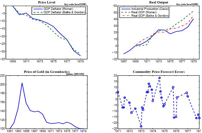
Figure 2.  The Deflation of 1920-21

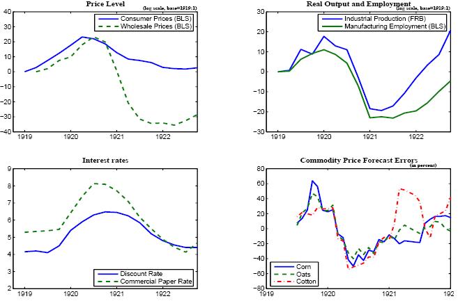
Figure 3.  The Volcker Disinflation

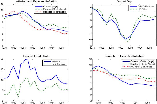
Figure 4.  The Evolution of Long-Term Bond Yields, 1867-1870

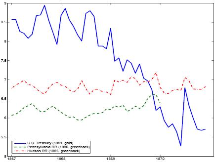
Figure 5.  Simulations of the Post-Civil War Episode

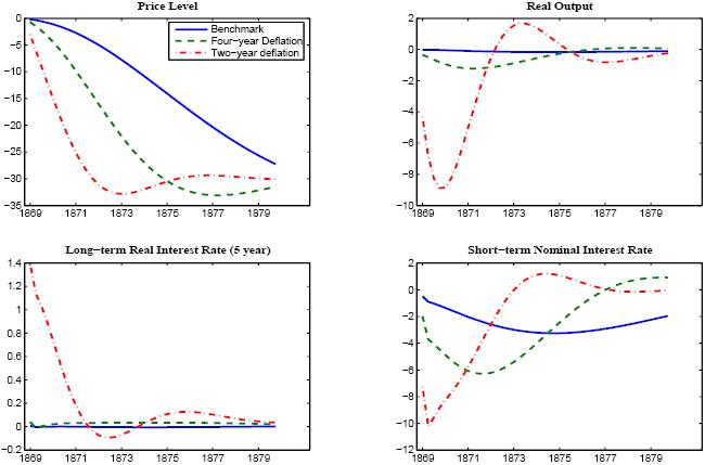
Figure 6.  Simulations of the Post-WWI Episode

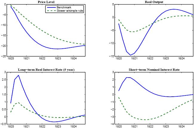
Figure 7.  The Estimated Policy Reaction Function during the Volcker Disinflation

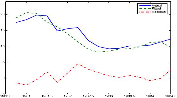
Figure 8.  Benchmark Simulation of the Volcker Disinflation

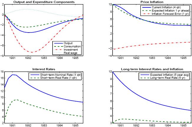
Figure 9.  Counterfactual Simulation of Volcker Disinflation under Complete Information

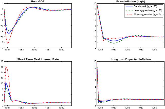
Figure 10.  Counterfactual Simulation of Volcker Disinflation under IncompleteInformation

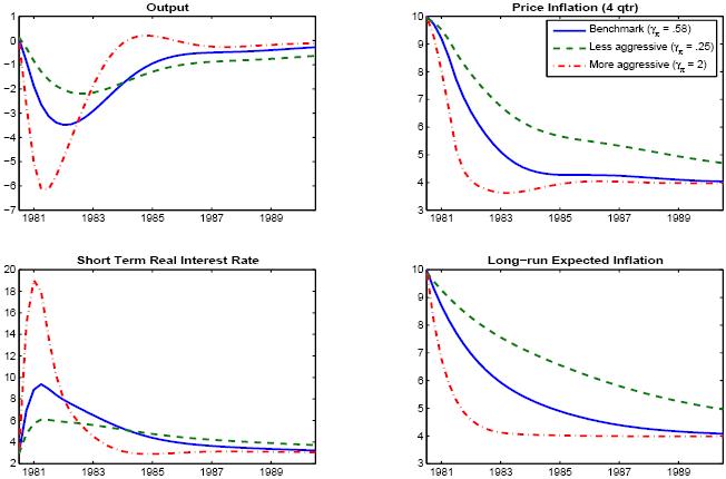
Footnotes

* Corresponding author: 20th and C Streets NW, Washington, DC 20051 USA; phone 202-452-2575; fax 202-872-4926; email [email protected]. Return to text

1.   Humphrey (2004) provides an excellent survey of the views of leading classical economists regarding the macroeconomic effects of deflation and the associated challenges for policymakers. Return to text

2.   For example, see Gordon (1982), Taylor (1983), and Ball (1994a). Return to text

3.   As seen in Figure 1, available output measures suggest that growth was relatively strong throughout the period surrounding the passage of the Public Credit Act in 1869. In particular, Davis' (2004) industrial production series (which is available prior to 1869, the year the GDP series begin) grows at about 6 percent per year between 1867 and 1873, notwithstanding about a 25 percent appreciation of the dollar relative to gold and major foreign currencies. Return to text

4.   The restoration of specie convertibility was supported by all three branches of government. It had the enthusiastic backing of the three successive Republican presidents who held office during the period (Johnson, Grant, and Hayes), and, through its decisions, the indirect support of the Supreme Court. While there was less unanimity in Congress, especially after the 1873 Panic, the debate hinged more on the appropriate speed of restoring convertibility at the official price, rather than on the ultimate goal.  Return to text

5.   There was admittedly some uncertainty about what the target for the dollar price of gold implied for the long-run price level, i.e., for how much price deflation would ultimately have to take place. However, while the real price of gold rose through the 1870s, it seems unlikely that this slow and steady rise significantly exacerbated the problem faced by private agents of making price-level forecasts to set the terms of multiperiod contracts.  Return to text

6.   While the war was primarily financed through higher taxes and the issuance of government bonds, money creation by the Federal Reserve System also played a significant role (Rockoff, 2005). Return to text

7.   Unlike the Civil war period, in which the dollar was allowed to float, the official price of gold remained fixed during WWI. Thus, the task facing policymakers was to ensure that gold reserves were sufficient to support free convertibility after the lifting of the embargo. Return to text

8.   The System's most potent policy instrument was the discount rate charged by the System's Reserve Banks to its member commercial banks on short-term loans. The Reserve Banks could request an adjustment in its discount rate, but the Board had to approve. Return to text

9.   While government statistics indicate a very sharp recession-with real GNP in 1921 nearly 15 percent lower than in the previous year-the analysis of Romer (1988) and Balke and Gordon (1989) indicates that real output declined by roughly 3 to 6 percent over the period from 1919 through 1921. Return to text

10.   For example, the National Industrial Conference Board estimated that nonagricultural employment contracted nearly 10 percent from 1919 through 1921. Return to text

11.   It is difficult to assess the magnitude of this premium, which presumably fluctuated considerably with the business cycle. However, for some quantitative guidance, it is useful to consider the period after Resumption in 1879, when both railroad bond interest rates and U.S. treasury bond rates were denominated in gold. In 1880, the risk spread on high quality railroad bonds appeared to be in the range of 100-150 basis points. For example, the average yield on the Chicago and Alton Railroad 7's maturing in 1893 was about 5.3 percent in 1880 (Macaulay Table A51), compared with a yield on U.S. treasury bonds (4-1/2s of 1891) of 4.1 percent (Homer and Sylla, 1996).  Return to text

12.   Futures prices were obtained from various issues of the Chicago Tribune. Realized prices were taken from the NBER's macro history database, and from annual reports of the Chicago Board of Trade. Return to text

13.   The HMS drew on two different measures of commodity prices: a Bureau of Labor Statistics index of wholesale commodity prices, and an alternative index produced by the trade publication Bradstreet's. Using the BLS measure apparently favored by HMS researchers, commodity prices were about 19 percent higher in March 1920 than in March 1919, and about 15 percent higher than in November 1918 (using Bradstreet's, commodity prices were 15 percent higher than in March 1919, and 9 percent higher than in November 1918).  Return to text

14.   Given that the HMS forecasters saw the adjustment of retail prices to lag that of commodity prices, retail prices were expected to fall through much of 1921 (e.g., Bullock, 1921), suggesting that ex ante real interest rates were expected to remain at very elevated levels.  Return to text

15.   The futures data on corn and oats are from the Annual Reports of the Chicago Board of Trade, as in Hamilton (1992). Cotton futures traded on the New York commodity futures exchange, with the data recorded in the Commercial and Financial Chronicle. Return to text

16.   See Svensson (2003) and Woodford (2003) for extensive discussions of the use of targeting rules to characterize monetary policy. Return to text

17.   It is worth noting that the optimal targeting rule implies a complicated underlying interest rate reaction function (see Woodford and Gianonni 2005). But at least for our baseline case of a very slow deflation, the targeting rule can be approximated fairly well by a simple instrument rule in which the ex post real interest rate responds to the price level gap and output gap.  Return to text

18.   In an earlier version of this paper, we attempted to account for the effects of the massive decline in government spending following the November 1918 armistice by including a sequence of contractionary government spending shocks. We found that the inclusion of these shocks markedly dampened the effects of the post-war monetary expansion on output. However, given that the government spending declines were concentrated in 1919, they had a small effect on the behavior of output and prices thereafter. Hence, given our focus on the period following the monetary contraction of early 1920, we have confined our attention to monetary shocks. Return to text

19.   These authors argued that inflation persistence was not structural, but due to uncertainty about the conduct of monetary policy. Cogley and Sargent (2001) present econometric evidence that inflation persistence is regime-dependent using a time-varying coefficients model.  Return to text

20.   For simplicity, the constant terms have been suppressed in equation 17. Return to text

21.   In this regression, the short-term nominal interest rate is measured by the federal funds rate, the steady-state real interest rate $\bar{r}$ is set to 3 percent (consistent with our specification of the discount factor $\beta$), steady-state output growth $\bar{g}$ is set to 2.5 percent, and the inflation target $\pi^{\ast}$ is specified as 4 percent over this sample period. Return to text

22.   We use the median of four-quarter ahead inflation forecasts taken from the Survey of Professional Forecasters; this series is plotted in Figure 4).  Return to text

23.   Christiano, Eichenbaum, and Evans (2005) argued that such a specification provides a much better account of investment dynamics in response to a monetary policy shock. Return to text

This version is optimized for use by screen readers. Descriptions for all mathematical expressions are provided in LaTex format. A printable pdf version is available. Return to text

Home | Economic research and data | Publications and education resources
Accessibility | Contact us
Last update: August 8, 2007