
Board of Governors of the Federal Reserve System
International Finance Discussion Papers
Number 924, March 2008--- Screen Reader
Version*
A Solution to the Default Risk-Business Cycle Disconnect*
NOTE: International Finance Discussion Papers are preliminary materials circulated to stimulate discussion and critical comment. References in publications to International Finance Discussion Papers (other than an acknowledgment that the writer has had access to unpublished material) should be cleared with the author or authors. Recent IFDPs are available on the Web at http://www.federalreserve.gov/pubs/ifdp/. This paper can be downloaded without charge from the Social Science Research Network electronic library at http://www.ssrn.com/.
Abstract:
Models of business cycles in emerging economies explain the negative correlation between country spreads and output by modeling default risk as an exogenous interest rate on working capital. Models of strategic default explain the cyclical properties of sovereign spreads by assuming an exogenous output cost of default with special features, and they underestimate debt-output ratios by a wide margin. This paper proposes a solution to this default risk-business cycle disconnect based on a model of sovereign default with endogenous output dynamics. The model replicates observed V-shaped output dynamics around default episodes, countercyclical sovereign spreads, and high debt ratios, and it also matches the variability of consumption and the countercyclical fluctuations of net exports. Three features of the model are key for these results: (1) working capital loans pay for imported inputs; (2) imported inputs support more efficient factor allocations than when these inputs are produced internally; and (3) default on the foreign obligations of firms and the government occurs simultaneously.
Keywords: Business cycles, sovereign default, emerging economies
JEL classification: E32, E44, F32, F34
1 Introduction
Three key empirical regularities characterize the relationship between sovereign debt and economic activity in emerging economies:
(1) Output displays V-shaped dynamics around default episodes. Recent default episodes have been associated with deep recessions. Arellano (2007) shows that GDP deviations from trend in the quarter in which default occurred were -14 percent in Argentina, -13 percent in Russia and -7 percent in Ecuador. Using quarterly data for 39 developing countries over the 1970-2005 period, Levy-Yeyati and Panizza (2006) show that the recessions associated with defaults tend to begin prior to the defaults and generally hit bottom when the defaults take place. Tomz and Wright's (2007) study of the history of defaults for industrial and developing countries during the period 1820-2004 reports that the frequency of defaults is at its maximum when output is at least 7 percent below trend. They also found, however, that some defaults occurred with less severe recessions, or when output is not below trend in annual data.
(2) Interest rates on sovereign debt and domestic output are negatively correlated. Neumeyer and Perri (2005) report that the cyclical correlations between these interest rates and GDP range from -0.38 to -0.7 in five emerging economies, with an average correlation of -0.55. Uribe and Yue (2006) report correlations for seven emerging economies ranging from zero to -0.8, with an average of -0.42.1
(3) External debt as a share of GDP is high on average, and high when countries default. Foreign debt was about a third of GDP on average over the 1998-2005 period for the entire group of emerging and developing countries as defined in IMF (2006). Within this group, the highly indebted poor countries had the highest average debt ratio at about 100 percent of GDP, followed by the Eastern European and Western Hemisphere countries, with averages of about 50 and 40 percent of GDP respectively. Reinhart et al. (2003) report that the external debt ratio during default episodes averaged 71 percent of GDP for all developing countries that defaulted at least once in the 1824-1999 period. The default episodes of recent years are in line with this estimate: Argentina defaulted in 2001 with a 64 percent debt ratio, and Ecuador and Russia defaulted in 1998 with debt ratios of 85 and 66 percent of GDP respectively.
These empirical regularities have proven difficult to explain. On one hand, quantitative business cycle models can account for the negative correlation between country interest rates and output if the interest rate on sovereign debt is introduced as the exogenous interest rate faced by a small open economy in which firms require working capital to pay the wages bill.2 On the other hand, quantitative models of sovereign default based on the classic setup of Eaton and Gersovitz (1981) can generate countercyclical sovereign spreads if the sovereign country faces stochastic shocks to an exogenous output endowment.3 These models require exogenous output costs of default with special features in order to support non-trivial levels of debt together with observed default frequencies, but even with these costs they either produce mean debt ratios under 10 percent of GDP or underestimate default probabilities by a wide margin.4 Thus, there is a crucial disconnect between business cycle models and sovereign default models: the former lack an explanation of the default risk premia that drive their findings, while the latter lack an explanation of the business cycle dynamics that are critical for their results.
The country risk-business cycle disconnect raises three important questions: Would a business cycle model with endogenous default risk still be able to explain the stylized facts that models with exogenous country risk have explained? Can a model of sovereign default with endogenous output dynamics produce the large output declines needed to support high ratios of defaultable debt as an equilibrium outcome? Would a model that endogenizes both country risk and output dynamics be able to mimic the V-shaped dynamics of output associated with defaults, and the countercyclical behavior of default risk?
This paper aims to answer these questions by studying the quantitative implications of a model of sovereign default with endogenous output fluctuations. The model borrows from the sovereign default literature the workhorse Eaton-Gersovitz recursive formulation of strategic default in which a sovereign borrower makes optimal default choices by comparing the payoffs of repayment and default. In addition, the model borrows from the business cycle literature a transmission mechanism that links default risk with economic activity via the financing cost of working capital. We extend the two classes of models (sovereign debt and business cycle models) by developing a framework in which the equilibrium dynamics of output and default risk are determined jointly, and influence each other via the interaction between foreign lenders, the domestic sovereign borrower, and domestic firms. In particular, a fall in productivity in our setup increases the likelihood of default and hence sovereign spreads, and this in turn increases the firms' financing costs leading to a further fall in output, which in turn feeds back into default incentives and sovereign spreads.
We demonstrate via numerical analysis that the model can explain the three key empirical regularities of sovereign debt mentioned earlier: The model mimics the V-shaped pattern of output dynamics around defaults with large recessions that hit bottom during defaults, yields countercyclical interest rates on sovereign debt, and supports high debt-GDP ratios on average and in default episodes. These results are obtained requiring only a small fraction of firms' factor costs to be paid with working capital (only 10 percent of the cost of imported inputs). Moreover, the model matches key business cycle features like the variability of consumption and the countercyclical behavior of net exports.
These results hinge on three key assumptions of the model: First, producers of final goods obtain working capital loans from abroad to finance purchases of imported intermediate goods. Second, these producers can choose optimally to employ domestic intermediate goods instead of imported inputs, but this shift entails an efficiency loss. Third, the government can divert the firms' repayment of working capital loans when it defaults on its own debt, so that both agents default on their foreign obligations at the same time, and the interest rates they face are equal at equilibrium.
The transmission mechanism that connects country risk and business cycles in our model operates as follows: Final goods producers maximize profits and choose optimally whether to use imported inputs or inputs produced in the domestic economy. These two inputs are perfect substitutes in the production technology, but imported inputs have a higher financing cost because they need to be paid in advance using working capital, while domestic inputs require costly reallocation of labor away from final goods production into intermediate goods production. Thus, a shift from imported to domestic inputs causes an efficiency loss in production of final goods due to the reallocation of labor.5
The choice of imported v. domestic inputs by final goods producers depends on the country interest rate (inclusive of default risk), which drives the financing cost of working capital, and on the state of total factor productivity (TFP). When the country has access to world financial markets, they choose imported intermediate goods if the country interest rate is low enough and/or TFP is high enough for the efficiency loss from using domestic inputs to exceed the higher financial cost of imported inputs. That is, final goods producers trade off the higher financing cost of imported inputs for the enhanced efficiency in the use of labor services (which are fully allocated to final goods production). In this situation, fluctuations in default risk affect the cost of working capital and thus induce fluctuations in factor demands and output. Conversely, above (below) a threshold value of the interest rate (TFP) firms choose to use domestic inputs because the financing cost of imported inputs exceeds the efficiency loss due to domestic labor reallocation, with labor services now being allocated to both final and intermediate goods production.
When the economy defaults, both the government and firms are excluded from world credit markets for some time, with an exogenous probability of re-entry as is common in the recent quantitative studies of sovereign default. Since the probability of default depends on whether the country's value of default is higher than that of repayment, there is feedback between the economic fluctuations induced by changes in interest rate premia, default probabilities, and country risk. In particular, rising country risk in the periods leading to a default causes a decline in economic activity as the firms' financing cost increases. In turn, the expectation of lower output at higher levels of country risk alters repayment incentives for the sovereign, affecting the equilibrium determination of default risk premia.
The transmission mechanism linking country risk and business cycles generates an endogenous output cost of default that is larger in " better" states of nature (i.e., increasing in the state of TFP). This result follows from the efficiency loss caused by the optimal shift from imported to domestic inputs when default takes place. Since default yields an effective financing cost of working capital loans that is too high for firms to employ foreign inputs, firms always use domestic inputs when the country is in financial autarky. Before default, however, if the interest rate is low enough and/or TFP is high enough, firms operate with imported inputs, and therefore final goods production is higher than in the default scenario, in which final goods producers shift to domestic inputs. Hence, the decline in GDP at the moment of default is higher the higher TFP was just before default, and the fraction of output loss caused by a default increases with TFP. This increasing output cost of default is a key feature of the model because it implies that the option to default brings more " state contingency" into the asset market, allowing the model to produce equilibria that support significantly higher mean debt ratios than those obtained in existing models of sovereign default.
The increasing output cost of default also implies that output can fall sharply when the economy defaults, and that, because this output drop is driven by an efficiency loss due to sectoral labor reallocation, part of the output collapse will appear as a drop in the Solow residual (i.e. the fraction of aggregate GDP not accounted for by capital and labor). This is consistent with the data of emerging economies in crisis showing that a large fraction of the output collapse is attributed to the Solow residual (see Meza and Quintin (2006) and Mendoza (2007)). Moreover, Benjamin and Meza (2007) show that in Korea's 1997 crisis, the productivity drop did follow from a sectoral reallocation of labor from more to less productive sectors.
Our treatment of the financing cost of working capital differs from the treatment in Neumeyer and Perri (2005) and Uribe and Yue (2006), both of which treat the interest rate on working capital as an exogenous variable set to match the interest rate on sovereign debt. In contrast, in our setup both interest rates are driven by endogenous sovereign risk. In addition, in the Neumeyer-Perri and Uribe-Yue models, working capital loans pay the wages bill in full, while in our model firms use working capital to pay only for a fraction of imported intermediate goods. This lower working capital requirement is desirable because, at standard labor income shares, working capital loans would need to be about 2/3rds of GDP to cover the wages bill, and this is difficult to reconcile with observed ratios of bank credit to the private sector as a share of output in emerging economies, which hover around 50 percent (including all credit to households and firms at all maturities, not just short-term revolving loans to firms).
The rest of the paper proceeds as follows: Section 2 presents the model. Section 3 explores the model's quantitative implications for a benchmark calibration. Section 4 conducts sensitivity analysis. Section 4 concludes.
2 A Model of Sovereign Default and Business Cycles
We study a dynamic stochastic general equilibrium model of sovereign default and business cycles. There are four groups of agents in the model, three in the "domestic" small open economy (households, firms, and the sovereign government) and one abroad (foreign lenders).
2.1 Households
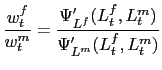
Households derive utility from consumption and disutility from
labor. Their preferences are given by a standard time-separable
utility function
![]() where
where ![]() is the discount factor, and
is the discount factor, and
![]() and
and ![]() denote
consumption and " composite" labor effort supplied in period
denote
consumption and " composite" labor effort supplied in period
![]() respectively.
respectively. ![]() is the
period utility function, which is continuous, strictly increasing,
strictly concave, and satisfies the Inada conditions. Following
Greenwood, Hercowitz and Huffman (1988), we remove the wealth
effect on labor supply by specifying period utility as a function
of consumption net of the disutility of labor
is the
period utility function, which is continuous, strictly increasing,
strictly concave, and satisfies the Inada conditions. Following
Greenwood, Hercowitz and Huffman (1988), we remove the wealth
effect on labor supply by specifying period utility as a function
of consumption net of the disutility of labor ![]() , where
, where ![]() is increasing,
continuously differentiable and convex. This formulation of
preferences has been shown to play an important role in allowing
international real business cycle models to explain observed
business cycle facts, and it also simplifies the supply-side of the
model by removing intertemporal considerations from the labor
supply choice.
is increasing,
continuously differentiable and convex. This formulation of
preferences has been shown to play an important role in allowing
international real business cycle models to explain observed
business cycle facts, and it also simplifies the supply-side of the
model by removing intertemporal considerations from the labor
supply choice.
Households choose consumption and sectoral allocations of labor
offered to producers of final goods and intermediate goods (
![]() and
and ![]() respectively). These sectoral labor supply allocations aggregate
into a composite amount of labor effort represented by a labor
transformation curve
respectively). These sectoral labor supply allocations aggregate
into a composite amount of labor effort represented by a labor
transformation curve
![]() , where
, where
![]() is a CES aggregator.
is a CES aggregator. ![]() and
and ![]() can thus be viewed as
efficiency units of labor that households allocate across the two
sectors out of a given amount of labor effort
can thus be viewed as
efficiency units of labor that households allocate across the two
sectors out of a given amount of labor effort ![]()
Households take as given the sectoral wage rates
![]() , the
profits paid by firms
, the
profits paid by firms
![]() and
government transfers
and
government transfers
![]() . Households do not
borrow directly from abroad, but they are still able to smooth
consumption because the government borrows, pays transfers, and
makes default decisions internalizing their utility function. This
assumption implies that the households' optimization problem
reduces to the following static problem:
. Households do not
borrow directly from abroad, but they are still able to smooth
consumption because the government borrows, pays transfers, and
makes default decisions internalizing their utility function. This
assumption implies that the households' optimization problem
reduces to the following static problem:
![$\displaystyle \max_{c_{t},L_{t}^{m},L_{t}^{f},L_{t}}E\left[ \sum\beta^{t}u\left( c_{t}-h\left( L_{t}\right) \right) \right]$](img19.gif)
|
(1) | ||
|
|
(2) | ||
| (3) |
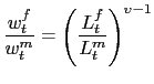
The optimality conditions for labor supply are:
| (4) | ||
| (5) |
Hence, optimal sectoral allocations of labor are obtained when the relative wage rates equal the sectoral marginal rate of transformation:
|
(6) |
The labor disutility function is defined in isoelastic form
![]() with
with
![]() The period utility function
takes the standard constant-relative-risk-aversion form
The period utility function
takes the standard constant-relative-risk-aversion form
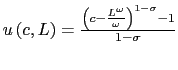 with
with ![]() . The labor transformation curve
is given by
. The labor transformation curve
is given by
![]() with
with
![]() .
.
![]() implies costless reallocation of
homogenous labor,
implies costless reallocation of
homogenous labor,
![]() and
and
![]() implies that the cost of
reallocating labor across sectors is infinite. With these
functional forms, the optimality condition for sectoral labor
supply allocations reduces to:
implies that the cost of
reallocating labor across sectors is infinite. With these
functional forms, the optimality condition for sectoral labor
supply allocations reduces to:
|
(7) |
Hence, the elasticity of substitution between ![]() and
and ![]() is equal to
is equal to
![]() .
.
2.2 Final Goods Producers
Firms are divided into a sector ![]() of final
goods producers and a sector
of final
goods producers and a sector ![]() of producers of
intermediate goods, both of which maximize profits. Firms in the
of producers of
intermediate goods, both of which maximize profits. Firms in the
![]() sector use labor and intermediate goods,
and face Markov TFP shocks
sector use labor and intermediate goods,
and face Markov TFP shocks
![]() with transition probability
distribution function
with transition probability
distribution function
![]() . The
production function of the
. The
production function of the ![]() sector is
Cobb-Douglas:
sector is
Cobb-Douglas:
| (8) |
with
![]() and
and
![]() .
.
The ![]() sector chooses optimally whether to import
intermediate goods from abroad or buy them from the
sector chooses optimally whether to import
intermediate goods from abroad or buy them from the ![]() sector at home. Imported inputs are sold in a competitive world
market at the exogenous relative price
sector at home. Imported inputs are sold in a competitive world
market at the exogenous relative price
![]() .6 A fraction
.6 A fraction ![]() of the cost of these imported inputs needs to be paid
in advance using working capital loans
of the cost of these imported inputs needs to be paid
in advance using working capital loans
![]() , which are intraperiod loans
repaid at the end of the period that are offered by foreign
creditors at the interest rate
, which are intraperiod loans
repaid at the end of the period that are offered by foreign
creditors at the interest rate ![]() . This interest
rate is linked to the sovereign interest rate at equilibrium, as
shown in the next section. Working capital loans satisfy the
standard payment-in-advance condition:
. This interest
rate is linked to the sovereign interest rate at equilibrium, as
shown in the next section. Working capital loans satisfy the
standard payment-in-advance condition:
| (9) |
Profit-maximizing firms choose
![]() so that this condition holds with
equality.
so that this condition holds with
equality.
The profits of final goods producers when they use imported inputs are:
| (10) |
Alternatively, when they use domestic intermediate goods, their profits are given by:
| (11) |
where ![]() is the endogenous price of intermediate
goods produced at home. As noted earlier, domestic inputs do not
require working capital financing. This assumption is just for
simplicity, the key element for the analysis is that at high levels
of country risk (including periods without access to foreign credit
markets) the financing cost of foreign inputs is higher than that
of domestic inputs.
is the endogenous price of intermediate
goods produced at home. As noted earlier, domestic inputs do not
require working capital financing. This assumption is just for
simplicity, the key element for the analysis is that at high levels
of country risk (including periods without access to foreign credit
markets) the financing cost of foreign inputs is higher than that
of domestic inputs.
Final goods producers maximize profits taking the sectoral wage rate, the interest rate, and intermediate goods prices as given, and choosing whether to use domestic or imported intermediate goods and the optimal amount of intermediate goods and labor to buy in each case. This is equivalent to first evaluating the profit-maximizing plans under each alternative (domestic v. imported inputs) and then choosing the one that yields higher profits:
![$\displaystyle \pi_{t}^{f}=\max\left[ \max_{m_{t},L_{t}^{f}}(\pi_{t}^{\ast}),\max _{m_{t},L_{t}^{f}}(\pi_{t}^{d})\right]$](img63.gif)
|
(12) |
When imported intermediate goods are used, the optimality conditions are
| (13) | ||
| (14) |
Alternatively, when domestic inputs are used, the optimality conditions are:
| (15) | ||
| (16) |
These two sets of optimality conditions are standard: Marginal products of factors of production equal the corresponding marginal costs.
2.3 Intermediate Goods Producers
Domestic inputs do not require advance payment, but in order to
produce them labor has to be reallocated from the ![]() sector to the
sector to the ![]() sector. At equilibrium, the
sector. At equilibrium, the ![]() sector operates only if the market price of its output is
positive, which occurs only if the
sector operates only if the market price of its output is
positive, which occurs only if the ![]() sector
chooses to use domestic inputs.
sector
chooses to use domestic inputs.
Producers in the ![]() sector operate with a
production function given by
sector operate with a
production function given by
![]() , with
, with ![]() and
and
![]() Given the domestic price of
intermediate goods and the sectoral wage rate, they choose labor
demand so as to solve the following profit maximization
problem:
Given the domestic price of
intermediate goods and the sectoral wage rate, they choose labor
demand so as to solve the following profit maximization
problem:
| (17) |
If sector ![]() producers find it optimal to use
imported inputs, the demand for domestic intermediate goods is
zero, and hence
producers find it optimal to use
imported inputs, the demand for domestic intermediate goods is
zero, and hence
![]() and
and ![]() are
zero and the
are
zero and the ![]() sector is idle. If final goods
producers demand domestic intermediate goods, optimal labor demand
by producers of intermediate goods satisfies
sector is idle. If final goods
producers demand domestic intermediate goods, optimal labor demand
by producers of intermediate goods satisfies
| (18) |
2.4 Competitive Equilibrium of the Private Sector
![$ \left[ c_{t},L_{t},L_{t}^{f},L_{t}^{m},m_{t} ,\kappa_{t}\right] _{t=0}^{\infty}$](img86.gif) and prices
and prices
![$ \left[ w_{t}^{f},w_{t} ^{m},p_{t}^{m},\pi_{t}^{f},\pi_{t}^{m}\right] _{t=0}^{\infty}$](img87.gif) such that:
such that:
1. The allocations
![$ \left[ c_{t},L_{t},L_{t}^{f},L_{t}^{m}\right] _{t=0}^{\infty}$](img88.gif) solve the households' utility maximization problem
solve the households' utility maximization problem![]()
2. The allocations
![$ \left[ L_{t}^{f},m_{t},\kappa_{t}\right] _{t=0}^{\infty }$](img90.gif) solve the profit maximization problem of sector
solve the profit maximization problem of sector ![]() producers.
producers.
3. The allocations
![]() solve
the profit maximization problem of sector
solve
the profit maximization problem of sector ![]() producers.
producers.
4. The labor market-clearing conditions hold.
Standard national income accounting implies that the economy's
GDP is equal to either: (a) the gross output of the ![]() sector net of the cost of imported inputs if final goods producers
use imported inputs, or (b) the gross output of the
sector net of the cost of imported inputs if final goods producers
use imported inputs, or (b) the gross output of the ![]() sector if final goods producers use domestic inputs. In the first
case, the
sector if final goods producers use domestic inputs. In the first
case, the ![]() sector is not operating and GDP at
factor costs follows from the definition of profits of the
sector is not operating and GDP at
factor costs follows from the definition of profits of the
![]() sector:
sector:
![]() . This excludes
. This excludes
![]() of gross output of final goods
because imports of intermediate goods are factor payments to
foreigners. In the second case, the definitions of profits of the
of gross output of final goods
because imports of intermediate goods are factor payments to
foreigners. In the second case, the definitions of profits of the
![]() and
and ![]() sectors yield:
sectors yield:
![]()
A key constraint on the problem of the sovereign borrower making
the default decision will be that the private-sector allocations
must be a competitive equilibrium. Since the sovereign government's
problem and the equilibrium of the credit market will be
characterized in recursive form, it is useful to also characterize
the allocations of the above competitive equilibrium in recursive
form (i.e. as functions defined in the state space domain). This is
done by first expressing the optimal allocations of labor and
intermediate goods when sector ![]() uses imported
inputs as the following functions of
uses imported
inputs as the following functions of ![]() and
and
![]() :
:
![$\displaystyle =\left[ \alpha_{L}^{\alpha_{L}}\left( \varepsilon k^{\alpha_{k}}\right) ^{\omega}\left( \frac{\alpha_{m}}{p_{m}^{\ast }(1+\theta r)}\right) ^{\omega-\alpha_{L}}\right] ^{\frac{1}{\omega\left( 1-\alpha_{m}\right) -\alpha_{L}}}$](img107.gif)
|
(19) | |
![$\displaystyle =\left[ \alpha_{L}\left( \varepsilon k^{\alpha_{k}}\right) ^{\frac{1}{1-\alpha_{m}}}\left( \frac{\alpha_{m} }{p_{m}^{\ast}(1+\theta r)}\right) ^{\frac{\alpha_{m}}{1-\alpha_{m}}}\right] ^{\frac{1-\alpha_{m}}{\omega\left( 1-\alpha_{m}\right) -\alpha_{L}} }$](img109.gif)
|
(20) |
If sector ![]() uses domestic inputs instead, the
optimal allocations of factors of production in the
uses domestic inputs instead, the
optimal allocations of factors of production in the ![]() and
and ![]() sectors are:
sectors are:
| (21) | ||
| (22) | ||
| (23) | ||
|
(24) |
where
 and
and
![]()
 . Note also that the equilibrium price of the domestic intermediate
goods is
. Note also that the equilibrium price of the domestic intermediate
goods is
![]()
![]()
It follows from the above solutions that final goods production
is not affected by foreign interest rates when firms use domestic
intermediate goods, because sector ![]() is not
borrowing from abroad in this case. In contrast, when producers of
final goods use imported inputs, their demand for these inputs and
labor decreases with
is not
borrowing from abroad in this case. In contrast, when producers of
final goods use imported inputs, their demand for these inputs and
labor decreases with ![]() . Thus, in this
situation, sovereign risk affects the actions of sector
. Thus, in this
situation, sovereign risk affects the actions of sector ![]() firms. Because, as we show later, the interest rate on
foreign working capital loans is driven by the sovereign interest
rate, these firms face higher financing costs when default risk
rises, and so their factor demands and output fall. One special
case of this situation is the state when default occurs, in which
the country has no access to working capital because effectively
firms. Because, as we show later, the interest rate on
foreign working capital loans is driven by the sovereign interest
rate, these firms face higher financing costs when default risk
rises, and so their factor demands and output fall. One special
case of this situation is the state when default occurs, in which
the country has no access to working capital because effectively
![]() has gone to infinity. In this case, firms
cannot import inputs from abroad and switch to use domestic
substitutes. Note, however, that the interest rate does not need to
rise to infinity for the switch to occur. Firms switch to domestic
inputs at a finite interest rate that is high enough for
has gone to infinity. In this case, firms
cannot import inputs from abroad and switch to use domestic
substitutes. Note, however, that the interest rate does not need to
rise to infinity for the switch to occur. Firms switch to domestic
inputs at a finite interest rate that is high enough for
![]() .
.
Next we define the indicator function
![]() to identify whether the
to identify whether the
![]() sector is using domestic or imported
inputs at the current state of interest rates and TFP. In
particular,
sector is using domestic or imported
inputs at the current state of interest rates and TFP. In
particular,
![]() if
if
![]() and
and
![]() if
if
![]() for a given
for a given
![]() pair. Hence, firms use
imported (domestic) inputs when
pair. Hence, firms use
imported (domestic) inputs when
![]() (
(
![]() ). The competitive
equilibrium allocations of factor demands and working capital can
now be expressed as functions of
). The competitive
equilibrium allocations of factor demands and working capital can
now be expressed as functions of ![]() and
and
![]() as follows:
as follows:
| (25) | ||
| (26) | ||
| (27) | ||
| (28) | ||
| (29) |
2.5 Endogenous Output Cost of Default
The decision by firms in the ![]() sector to shift
between foreign and domestic inputs depends on the states of the
interest rate and TFP. The mechanism that drives this shift can be
illustrated by examining the
sector to shift
between foreign and domestic inputs depends on the states of the
interest rate and TFP. The mechanism that drives this shift can be
illustrated by examining the ![]() sector firms'
optimal choice of intermediate goods using Figure 1. For
simplicity, we draw this figure assuming that total labor effort
sector firms'
optimal choice of intermediate goods using Figure 1. For
simplicity, we draw this figure assuming that total labor effort
![]() is inelastic. The demand for intermediate
goods is determined by the marginal product of
is inelastic. The demand for intermediate
goods is determined by the marginal product of ![]() .
The corresponding marginal productivity curve when foreign
(domestic) inputs are used is labeled
.
The corresponding marginal productivity curve when foreign
(domestic) inputs are used is labeled
![]() (
(
![]() ). The marginal
productivity of intermediate goods employed in final goods
production is always lower when domestic inputs are used, because
of the reallocation of labor from final goods production to
production of intermediate goods. Given the Cobb-Douglas production
function for
). The marginal
productivity of intermediate goods employed in final goods
production is always lower when domestic inputs are used, because
of the reallocation of labor from final goods production to
production of intermediate goods. Given the Cobb-Douglas production
function for ![]() , the lower labor input available to
the
, the lower labor input available to
the ![]() sector when it uses domestic inputs
reduces the marginal product of intermediate goods in production of
final goods.7 Moreover, because the reallocation of
labor is costly, one unit of labor taken away from the
sector when it uses domestic inputs
reduces the marginal product of intermediate goods in production of
final goods.7 Moreover, because the reallocation of
labor is costly, one unit of labor taken away from the ![]() sector yields less than one unit of labor in the
sector yields less than one unit of labor in the
![]() sector, and the higher this reallocation
cost the lower the marginal product of domestic intermediate goods
relative to that of imported intermediate goods (i.e. the larger
the gap between
sector, and the higher this reallocation
cost the lower the marginal product of domestic intermediate goods
relative to that of imported intermediate goods (i.e. the larger
the gap between
![]() and
and
![]() ).
).
Figure 1: The Intermediate Goods Market
The supply of imported inputs is infinitely elastic at an
exogenous price
![]() . In contrast, the
supply of domestic inputs (
. In contrast, the
supply of domestic inputs ( ![]() in Figure 1)
is determined by the production plans of the
in Figure 1)
is determined by the production plans of the ![]() sector. This supply function is given by
sector. This supply function is given by
 .
.
If the interest rate is sufficiently low, the firms' optimal
plans call for using imported inputs up to the amount at which the
marginal product of ![]() equals the marginal cost
equals the marginal cost
![]() . This is point A in
Figure 1. Around point A, output fluctuates as a result of changes
in
. This is point A in
Figure 1. Around point A, output fluctuates as a result of changes
in ![]() and
and
![]() . Consider first the interest
rate. Given that marginal products are decreasing and continuously
differentiable, it follows that as
. Consider first the interest
rate. Given that marginal products are decreasing and continuously
differentiable, it follows that as ![]() rises the
demand for imported inputs and the profits of final goods producers
decline, until we reach a threshold value
rises the
demand for imported inputs and the profits of final goods producers
decline, until we reach a threshold value
![]() at which
at which
![]()
![]() is an interest rate high enough
for these producers to find it optimal to switch to the domestic
inputs, because
is an interest rate high enough
for these producers to find it optimal to switch to the domestic
inputs, because
![]() yields
yields
![]() . This threshold point
is shown as point C in Figure 1.
. This threshold point
is shown as point C in Figure 1.
When the interest rate reaches
![]() , final goods producers switch to
domestic inputs and the equilibrium price and quantity of
intermediate goods are determined at point B. Notice that, because
imported inputs have higher marginal product, when interest rates
are high (but not yet at
, final goods producers switch to
domestic inputs and the equilibrium price and quantity of
intermediate goods are determined at point B. Notice that, because
imported inputs have higher marginal product, when interest rates
are high (but not yet at
![]() ) it can be optimal for firms to
use quantities of imported inputs that are lower than what they use
if they operate with domestic inputs (
) it can be optimal for firms to
use quantities of imported inputs that are lower than what they use
if they operate with domestic inputs (![]() ). This
is because in this situation firms still make more profits with the
foreign inputs than by switching to domestic inputs.
). This
is because in this situation firms still make more profits with the
foreign inputs than by switching to domestic inputs.
Around point B, fluctuations in output are driven by changes in
![]() but output is no longer
affected by the interest rate. This has two important implications.
First, since in principle
but output is no longer
affected by the interest rate. This has two important implications.
First, since in principle
![]() can be reached before the country
defaults, high interest rates can trigger a switch to domestic
inputs even before default occurs. Second, since
can be reached before the country
defaults, high interest rates can trigger a switch to domestic
inputs even before default occurs. Second, since
![]() is well defined and at default
is well defined and at default
![]() , firms always use
domestic inputs when the economy defaults.
, firms always use
domestic inputs when the economy defaults.
Productivity shocks can also cause the switch from imported to
domestic inputs, even if ![]() remains constant. As with
the interest rate, there is a threshold TFP level at which final
goods producers are indifferent between using imported or domestic
inputs because
remains constant. As with
the interest rate, there is a threshold TFP level at which final
goods producers are indifferent between using imported or domestic
inputs because
![]()
![]() . For
TFP shocks below this threshold, these producers opt for domestic
inputs. The reason is that a low
. For
TFP shocks below this threshold, these producers opt for domestic
inputs. The reason is that a low
![]() lowers the marginal product of
imported inputs but firms still pay the extra marginal cost due to
the cost of working capital. Hence, firms choose to use domestic
inputs (and bear the efficiency loss) rather than paying this
financing cost.
lowers the marginal product of
imported inputs but firms still pay the extra marginal cost due to
the cost of working capital. Hence, firms choose to use domestic
inputs (and bear the efficiency loss) rather than paying this
financing cost.
The switch from imported to domestic inputs that occurs at high
interest rates has important implications for the output cost of
default. In particular, it makes the cost of default an increasing
function of the state of TFP. This property of the default cost can
be illustrated by studying how productivity shocks affect the
fraction of GDP lost in a default
![]() where
where ![]() and
and ![]() represent GDP when the
economy has access to credit markets and when the economy defaults
respectively (both given by the fraction
represent GDP when the
economy has access to credit markets and when the economy defaults
respectively (both given by the fraction
![]() of
final goods production.
of
final goods production.
Figure 2 shows how ![]()
![]() and the output loss at default change with TFP shocks
for a given
and the output loss at default change with TFP shocks
for a given ![]() . If the country defaults, exclusion
from world credit markets prevents final goods producers from
accessing working capital loans and forces them to switch to
domestic inputs, so along the
. If the country defaults, exclusion
from world credit markets prevents final goods producers from
accessing working capital loans and forces them to switch to
domestic inputs, so along the ![]() line firms
always operate with domestic inputs. If the country has access to
world credit markets, final goods producers choose optimally
whether to use imported or domestic inputs. Hence,
line firms
always operate with domestic inputs. If the country has access to
world credit markets, final goods producers choose optimally
whether to use imported or domestic inputs. Hence, ![]() is produced with imported inputs as long as
is produced with imported inputs as long as
![]() is above the threshold at which
final goods producers switch to domestic inputs, and
is above the threshold at which
final goods producers switch to domestic inputs, and
![]() otherwise.
otherwise.
Figure 2: Output and the Output Cost of Default as Functions of TFP
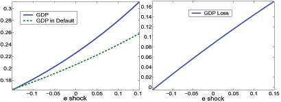
Data for Figure 2
e shock | GDP | GDP in default | GDP_loss |
|---|---|---|---|
-0.1500 | 0.1638 | 0.1647 | 0.2960 |
-0.1342 | 0.1694 | 0.1686 | 0.3031 |
-0.1184 | 0.1752 | 0.1727 | 0.3102 |
-0.1026 | 0.1812 | 0.1768 | 0.3171 |
-0.0868 | 0.1875 | 0.1810 | 0.3240 |
-0.0711 | 0.1939 | 0.1854 | 0.3309 |
-0.0553 | 0.2006 | 0.1898 | 0.3376 |
-0.0395 | 0.2075 | 0.1944 | 0.3443 |
-0.0237 | 0.2147 | 0.1990 | 0.3509 |
-0.0079 | 0.2220 | 0.2038 | 0.3575 |
0.0079 | 0.2297 | 0.2087 | 0.3640 |
0.0237 | 0.2376 | 0.2137 | 0.3704 |
0.0395 | 0.2458 | 0.2188 | 0.3768 |
0.0553 | 0.2542 | 0.2241 | 0.3831 |
0.0711 | 0.2630 | 0.2294 | 0.3893 |
0.0868 | 0.2720 | 0.2349 | 0.3955 |
0.1026 | 0.2814 | 0.2406 | 0.4016 |
0.1184 | 0.2911 | 0.2463 | 0.4076 |
0.1342 | 0.3011 | 0.2522 | 0.4136 |
0.1500 | 0.3114 | 0.2583 | 0.4195 |
As Figure 2 shows, the output cost of default increases with the
size of the TFP shock, because default is accompanied by a switch
from ![]() to
to ![]() so
default is more painful at higher levels of TFP. This property of
the output cost of default is key for the model's ability to
support high debt levels together with observed default
frequencies, because it makes the default option more attractive to
the country at lower states of productivity, and works as a
desirable implicit hedging mechanism given the incompleteness of
asset markets.
so
default is more painful at higher levels of TFP. This property of
the output cost of default is key for the model's ability to
support high debt levels together with observed default
frequencies, because it makes the default option more attractive to
the country at lower states of productivity, and works as a
desirable implicit hedging mechanism given the incompleteness of
asset markets.
This finding is in line with Arellano's (2007) result showing that an exogenous default cost with similar features can allow the Eaton-Gersovitz model to support non-trivial levels of debt together with observed default frequencies. In particular, she proposed an exogenous default cost function such that below a threshold level of an output endowment default does not entail an output cost, but above that threshold default reduces the endowment to a state-invariant fraction of the long-run average of GDP. In this second range, the size of the output loss is increasing in the output realization at the time of default. Still, the mean debt ratio in her baseline calibration was only about 6 percent of GDP (assuming output at default is 3 percent below mean output), while we show later that our model with an endogenous output cost of default yields a mean debt ratio about four times larger.
2.6 The Sovereign Government
The sovereign government trades with foreign lenders one-period,
zero-coupon discount bonds, so markets of contingent claims are
incomplete. The face value of these bonds specifies the amount to
be repaid next period and is denoted as ![]() . When
the country purchases bonds
. When
the country purchases bonds ![]() , and
when it borrows
, and
when it borrows ![]() . The set of bond face
values is
. The set of bond face
values is
![]() , where
, where
![]() . We set the lower
bound
. We set the lower
bound
![]() , which
is the largest debt that the country could repay with full
commitment. The upper bound
, which
is the largest debt that the country could repay with full
commitment. The upper bound ![]() is the
highest level of assets that the country may accumulate.8
is the
highest level of assets that the country may accumulate.8
The sovereign cannot commit to repay its debt. As in the
Eaton-Gersovitz model, we assume that when the country defaults it
does not repay at date ![]() and the punishment is
exclusion from the world credit market in the same period. The
country re-enters the credit market with an exogenous probability
and the punishment is
exclusion from the world credit market in the same period. The
country re-enters the credit market with an exogenous probability
![]() , and when it does it starts with a
fresh record and zero debt.9 Also as in the Eaton-Gersovitz
setup, the country cannot hold positive international assets during
the exclusion period, otherwise the model cannot support equilibria
with debt.
, and when it does it starts with a
fresh record and zero debt.9 Also as in the Eaton-Gersovitz
setup, the country cannot hold positive international assets during
the exclusion period, otherwise the model cannot support equilibria
with debt.
We add to the Eaton-Gersovitz setup an explicit link between default risk and private financing costs. This is done by assuming that a defaulting sovereign can divert the repayment of the firms' working capital loans to foreign lenders. Hence, both firms and government default together. This is perhaps an extreme formulation of the link between private and public borrowing costs, but we provide later some evidence in favor of this view.
The sovereign government solves a problem akin to a Ramsey
problem.10 It chooses a debt policy (amounts
and default) that maximizes the households' welfare subject to the
constraints that: (a) the private sector allocations must be a
competitive equilibrium; and (b) the government budget constraint
must hold. The state variables are the initial foreign asset
position, working capital loans as of the end of last period, and
the state of TFP, denoted by the triplet
![]() . The price
of sovereign bonds is given by the bond pricing function
. The price
of sovereign bonds is given by the bond pricing function
![]() .
Since at equilibrium the default risk premium on sovereign debt
will be the same as on working capital loans, it follows that the
interest rate on working capital is a function of
.
Since at equilibrium the default risk premium on sovereign debt
will be the same as on working capital loans, it follows that the
interest rate on working capital is a function of
![]() .
Hence, the recursive expressions that represent the competitive
equilibrium of the private sector derived earlier can be expressed
as as
.
Hence, the recursive expressions that represent the competitive
equilibrium of the private sector derived earlier can be expressed
as as
![]() ,
,
![]()
![]()
![]() ,
,
![]() , and
, and
![]() .
.
The recursive optimization problem of the government is summarized by the following value function:
![$\displaystyle V\left( b_{t},\kappa_{t-1},\varepsilon_{t}\right) =\left\{ \begin{array}[c]{ll} \max\left\{ v^{nd}\left( b_{t},\varepsilon_{t}\right) ,v^{d}\left( \kappa_{t-1,}\varepsilon_{t}\right) \right\} & \text{for }b_{t}<0\\ v^{nd}\left( b_{t},\varepsilon_{t}\right) & \text{for }b_{t}\geq0 \end{array} \right.$](img227.gif)
|
(30) |
If the country has access to the world credit market at date
![]() , the value function is the maximum of the
value of continuing in the credit relationship with foreign lenders
(i.e., repayment or "no default"),
, the value function is the maximum of the
value of continuing in the credit relationship with foreign lenders
(i.e., repayment or "no default"),
![]() ,
and the value of default,
,
and the value of default,
![]() . If the
economy holds a non-negative net foreign asset position, the value
function is simply the continuation value because in this case the
economy is using the credit market to save, receiving a return
equal to the world's risk free rate
. If the
economy holds a non-negative net foreign asset position, the value
function is simply the continuation value because in this case the
economy is using the credit market to save, receiving a return
equal to the world's risk free rate ![]() .
.
The continuation value
![]() is defined as follows:
is defined as follows:
![$\displaystyle v^{nd}\left( b_{t},\varepsilon_{t}\right) =\underset{c_{t},b_{t+1}}{\max }\left\{ \begin{array}[c]{c} u\left( c_{t}-h(L\left( q_{t}\left( b_{t+1},\varepsilon_{t}\right) ,\varepsilon_{t}\right) )\right) \;\;\;\;\;\;\;\;\;\;\;\;\;\;\;\;\;\;\;\;\;\;\;\\ \;\;\;\;\;\;\;+\beta E\left[ V\left( b_{t+1},\kappa\left( q_{t}\left( b_{t+1},\varepsilon_{t}\right) ,\varepsilon_{t}\right) ,\varepsilon _{t+1}\right) \right] \end{array} \right\}$](img233.gif)
|
(31) |
subject to
| (32) |
The constraint of this problem is the resource constraint of the
economy at a competitive equilibrium. The left-hand-side is the sum
of consumption and net exports, and the right-hand-side is GDP.
This constraint is obtained by combining the households' budget
constraint (2) with the government budget constraint,
![]() , and noting that the firms' optimality conditions imply that total
domestic factor payments,
, and noting that the firms' optimality conditions imply that total
domestic factor payments,
![]() , equal the fraction
, equal the fraction
![]() of gross
output of final goods
of gross
output of final goods
![]()
The resource constraint captures three important features of the
model: First, the government internalizes how interest rates affect
the competitive equilibrium allocations of output and factor
demands. Second, the households cannot borrow from abroad, but the
government internalizes their desire to smooth consumption and
transfers to them an amount equal to the negative of the balance of
trade (i.e. it gives the private sector the flow of resources it
needs to finance the gap between GDP and consumption). Third, the
working capital loans
![]() and
and
![]() do not enter explicitly in the
continuation value or in the resource constraint, because working
capital payments are included in the fraction of gross output
allocated to payments of intermediate goods,
do not enter explicitly in the
continuation value or in the resource constraint, because working
capital payments are included in the fraction of gross output
allocated to payments of intermediate goods,
![]() . Still, we need to
keep track of the state variable
. Still, we need to
keep track of the state variable
![]() because the amount of working
capital loans taken by final goods producers at date
because the amount of working
capital loans taken by final goods producers at date ![]() affects the sovereign's incentive to default at
affects the sovereign's incentive to default at ![]() as explained below.
as explained below.
The value of
default
![]() is:
is:
![$\displaystyle v^{d}\left( \kappa_{t-1},\varepsilon_{t}\right) =\max_{c_{t}}\left\{ \begin{array}[c]{c} u\left( c_{t}-h(L(\varepsilon_{t}))\right) \;\ \ \ \ \ \ \ \ \ \ \ \ \ \ \ \;\;\;\;\;\;\;\;\;\;\;\;\;\;\;\;\;\;\;\;\;\;\;\;\;\;\;\;\;\;\;\;\;\;\\ \;\ \;\;\;\;\;\;\;\;\ \ \ \ \ \ \ \ +\beta\left( 1-\eta\right) Ev^{d}\left( 0,\varepsilon_{t+1}\right) +\beta\eta EV\left( 0,0,\varepsilon_{t+1}\right) \end{array} \right\}$](img247.gif)
|
(33) |
subject to:
| (34) |
Note that
![]() takes into
account the fact that in case of default at date
takes into
account the fact that in case of default at date ![]() the country has no access to financial markets this
period, and hence the country consumes the total income given by
the resource constraint in the default scenario. In this case,
since firms cannot borrow to finance purchases of imported inputs,
the country has no access to financial markets this
period, and hence the country consumes the total income given by
the resource constraint in the default scenario. In this case,
since firms cannot borrow to finance purchases of imported inputs,
![]() ,
, ![]() and
and
![]() are the
competitive equilibrium allocations that correspond to the case
when the
are the
competitive equilibrium allocations that correspond to the case
when the ![]() sector operates with domestic inputs.
Moreover, because the defaulting government diverts the repayment
of last period's working capital loans, total household income
includes government transfers equal to the appropriated repayment
for the amount
sector operates with domestic inputs.
Moreover, because the defaulting government diverts the repayment
of last period's working capital loans, total household income
includes government transfers equal to the appropriated repayment
for the amount
![]() (i.e., on the date of default,
the government budget constraint is
(i.e., on the date of default,
the government budget constraint is
![]() ). The value of default at
). The value of default at
![]() also takes into account that at
also takes into account that at
![]() the economy may re-enter world capital
markets with probability
the economy may re-enter world capital
markets with probability ![]() and associated value
and associated value
![]() , or
remain in financial autarky with probability
, or
remain in financial autarky with probability ![]() and associated value
and associated value
![]() .
.
For a debt position ![]() and given a level
of working capital
and given a level
of working capital
![]() , default is optimal for the set
of realizations of the TFP shock for which
, default is optimal for the set
of realizations of the TFP shock for which
![]() is at least
as high as
is at least
as high as
![]() :
:
| (35) |
It is critical to note that this default set has a different
specification than in the typical Eaton-Gersovitz model of
sovereign default (see Arellano (2007)), because the state of
working capital affects the gap between the values of default and
repayment. This results in a two-dimensional default set that
depends on ![]() and
and
![]() , instead of just
, instead of just ![]()
Despite the fact that the default set depends on
![]() , the probability of default
remains a function of
, the probability of default
remains a function of ![]() and
and
![]() only. This is because the
only. This is because the
![]() sector's optimality conditions imply that
the next period's working capital loan
sector's optimality conditions imply that
the next period's working capital loan
![]() depends on
depends on
![]() and the interest rate,
which is a function of
and the interest rate,
which is a function of ![]() and
and
![]() . Thus the probability of
default at
. Thus the probability of
default at ![]() perceived as of date
perceived as of date ![]() for a country with a productivity
for a country with a productivity
![]() and debt
and debt ![]() ,
,
![]() ,
can be induced from the default set, the decision rule for working
capital, and the transition probability function of productivity
shocks
,
can be induced from the default set, the decision rule for working
capital, and the transition probability function of productivity
shocks
![]() as
follows:
as
follows:
|
(36) | |
| where |
(37) |
The economy is considered to be in financial autarky when it has
been in default for at least one period and remains without access
to world credit markets as of date ![]() As noted
above, the economy can exit this exclusion stage at date
As noted
above, the economy can exit this exclusion stage at date
![]() with probability
with probability ![]() . We
assume that during the exclusion stage the economy cannot build up
its own stock of savings to supply working capital loans to firms,
which could be used to purchase imported inputs.11 This
assumption ensures that, as long as the economy remains in
financial autarky, the optimization problem of the sovereign is the
same as the problem in the default period but evaluated at
. We
assume that during the exclusion stage the economy cannot build up
its own stock of savings to supply working capital loans to firms,
which could be used to purchase imported inputs.11 This
assumption ensures that, as long as the economy remains in
financial autarky, the optimization problem of the sovereign is the
same as the problem in the default period but evaluated at
![]() (i.e.
(i.e.
![]() ).
).
We also studied an alternative setup in which we allowed for a domestic financial market to operate during the exclusion stage. In this case, households make saving plans to offer working capital loans to firms at a market-determined interest rate, and firms demand these loans if the endogenous domestic interest rate is low enough to make productions plans using foreign inputs more profitable than with domestic inputs, despite the higher financing cost of the former. In this case, domestic loans are included as an additional state variable and their interest rate is determined as an equilibrium outcome. We found, however, that for parameter values around our baseline calibration this domestic financial market is not viable: The interest rate at which households would find it optimal to accumulate savings is too high for firms to optimally choose to obtain domestic working capital loans to purchase imported inputs, instead of just using domestic inputs. Hence, the equilibrium for the model with the domestic financial market operating during the exclusion stage is the same as that for the model that simply assumes that firms operate with domestic inputs whenever they cannot access world credit markets.
The model preserves a standard feature of the Eaton-Gersovitz
model: Given
![]() , the value of defaulting is
independent of the level of debt, while the value of not defaulting
increases with
, the value of defaulting is
independent of the level of debt, while the value of not defaulting
increases with ![]() , and consequently the
default set and the equilibrium default probability grow with the
country's debt. The following theorem formalizes this result:
, and consequently the
default set and the equilibrium default probability grow with the
country's debt. The following theorem formalizes this result:
Proof. See Appendix.
2.7 Foreign Lenders
International creditors are risk-neutral and have complete information. They invest in sovereign bonds and in private working capital loans. Foreign lenders behave competitively and face an opportunity cost of funds equal to the world risk-free interest rate. Competition implies that they expect zero profits at equilibrium, and that the returns on sovereign debt and the world's risk-free asset are fully arbitraged:
![$\displaystyle q_{t}\left( b_{t+1},\varepsilon_{t}\right) =\left\{ \begin{array}[c]{cc} \frac{1}{1+r^{\ast}} & \text{if }b_{t+1}\geq0\\ \frac{\left[ 1-p_{t}\left( b_{t+1},\varepsilon_{t}\right) \right] }{1+r^{\ast}} & \text{if }b_{t+1}<0 \end{array} \right.$](img304.gif)
|
(38) |
This condition implies that at equilibrium bond prices depend on the risk of default. For a high level of debt, the default probability is higher. Therefore, equilibrium bond prices decrease with indebtedness. This result, formalized in Theorem 2 below, is consistent with the empirical evidence documented by Edwards (1984).
Proof. See Appendix.
The returns on sovereign bonds and working capital loans are also fully arbitraged. Because the sovereign government diverts the repayment of working capital loans when it defaults, foreign lenders assign the same risk of default to private working capital loans as to sovereign debt, and hence the no- arbitrage condition between sovereign lending and working capital loans implies:
 , if
, if |
(39) |
2.8 Country Risk & Private Interest Rates: Some Empirical Evidence
The result that the interest rates on sovereign debt and private working capital loans are the same raises a key empirical question: Are sovereign interest rates and the rates of interest faced by private firms closely related in emerging economies?
Providing a complete answer to this question is beyond the scope of this paper, but we do provide empirical evidence suggesting that indeed interest rates on loans to private firms and on sovereign bonds move together. To study this issue, we constructed country estimates of firms' financing costs that aggregate measures derived from firm-level data. We constructed a measure of firm-level effective interest rates as the ratio of a firm's total debt service divided by its total debt obligations using the Worldscope database, which provides the main lines of balance-sheet and cash-flow statements of publicly listed corporations. We then constructed the corresponding aggregate country measure as the median across firms.
Table 1: Sovereign Interest Rates and Firm Financing Cost
| Country | Sovereign Interest Rates | Median Firm Interest Rates | Correlation |
|---|---|---|---|
| Argentina | 13.32 | 10.66 | 0.87 |
| Brazil | 12.67 | 24.60 | 0.14 |
| Chile | 5.81 | 7.95 | 0.72 |
| China | 6.11 | 5.89 | 0.52 |
| Colombia | 9.48 | 19.27 | 0.86 |
| Egypt | 5.94 | 8.62 | 0.58 |
| Malaysia | 5.16 | 6.56 | 0.96 |
| Mexico | 9.40 | 11.84 | 0.74 |
| Morocco | 9.78 | 13.66 | 0.32 |
| Pakistan | 9.71 | 12.13 | 0.84 |
| Peru | 9.23 | 11.42 | 0.72 |
| Philippines | 8.78 | 9.27 | 0.34 |
| Poland | 7.10 | 24.27 | 0.62 |
| Russia | 15.69 | 11.86 | -0.21 |
| South Africa | 5.34 | 15.19 | 0.68 |
| Thailand | 6.15 | 7.30 | 0.94 |
| Turkey | 9.80 | 29.26 | 0.88 |
| Venezuela | 14.05 | 19.64 | 0.16 |
The comparison of this measure of interest rates faced by private firms with the standard EMBI+ measure of interest rates on sovereign debt shows two striking facts (see Table 1): First, the two interest rates are positively correlated in most countries, with a median correlation of 0.7, and in some countries the relationship is very strong (see Figure 3).12 Second, the effective financing cost of firms is generally higher than the sovereign interest rates. This fact indicates that the common conjecture that firms (particularly the large corporations covered in our data) may pay lower rates than governments with default risk is incorrect.
The study by Arteta and Hale (2007) provides further and more systematic evidence on the strong effects of sovereign debt on the terms of private-sector debt contracts of emerging economies. In particular, they show strong, systematic negative effects on private corporate bond issuance during and after default episodes.
Figure 3: Sovereign Bond Interest Rates and Median Firm Financing Costs
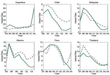
________ Sovereign Bond Interest Rates
----------- Median Firm Financing Cost
Data for Figure 3
Year | Argentina: Firm | Argentina: Sovereign | Chile: Firm | Chile: Sovereign | Malaysia: Firm | Malaysia: Sovereign | Mexico: Firm | Mexico: Sovereign | Peru: Firm | Peru: Sovereign | Thailand: Firm | Thailand: Sovereign |
|---|---|---|---|---|---|---|---|---|---|---|---|---|
| 1994 | 8.05 |
12.87 |
- |
- |
- |
- |
7.78 |
10.84 |
- |
- |
- |
- |
| 1995 | 7.18 |
18.24 |
- |
- |
- |
- |
17.43 |
17.13 |
- |
- |
- |
- |
| 1996 | 9.33 |
13.81 |
- |
- |
- |
- |
14.64 |
13.61 |
- |
- |
- |
- |
| 1997 | 9.08 |
10.13 |
- |
- |
6.58 |
6.92 |
11.28 |
10.08 |
9.99 |
10.03 |
7.64 |
7.86 |
| 1998 | 9.02 |
11.07 |
- |
- |
9 |
10.04 |
12.3 |
10.92 |
9.5 |
10.74 |
9.29 |
12.65 |
| 1999 | 10.55 |
12.57 |
8.67 |
7.33 |
8.29 |
9.38 |
13.1 |
11.83 |
11.29 |
11.51 |
7.78 |
10.2 |
| 2000 | 10.92 |
12.26 |
8.8 |
8.05 |
6.91 |
8.25 |
12.93 |
9.66 |
11.3 |
11.5 |
7.75 |
8.17 |
| 2001 | 13.76 |
15.64 |
8.18 |
6.53 |
6.87 |
7 |
11.83 |
8.42 |
10.7 |
11.15 |
6.15 |
7.17 |
| 2002 | 20.01 |
61.44 |
6.79 |
5.65 |
6.19 |
5.69 |
9.14 |
7.06 |
9.36 |
9.88 |
4.83 |
5.49 |
| 2003 | - |
- |
6.14 |
4.38 |
5.73 |
4.67 |
9.79 |
5.63 |
7.09 |
7.78 |
3.97 |
4.41 |
| 2004 | - |
- |
5.79 |
4.29 |
5.33 |
4.54 |
10.13 |
5.37 |
7.53 |
7 |
4.15 |
3.83 |
| 2005 | - |
- |
6.17 |
4.67 |
5.32 |
4.9 |
11.72 |
5.65 |
9.74 |
6.05 |
4.6 |
4.32 |
There is also evidence suggesting that our assumption that the government can divert the repayment of the firms' foreign obligations is realistic. In particular, it is not uncommon for the government to take over the foreign obligations of the corporate sector in actual default episodes. The following quote by the IMF historian explains how this was done in Mexico's 1982-83 default, and notes that arrangements of this type have been commonly used since then:
"A simmering concern among Mexico's commercial bank creditors was the handling of private sector debts, a substantial portion of which was in arrears...the banks and some official agencies had pressured the Mexican government to assume these debts...Known as the FICORCA scheme, this program provided for firms to pay dollar-denominated commercial debts in pesos to the central bank. The creditor was required to reschedule the debts over several years, and the central bank would then guarantee to pay the creditor in dollars. Between March and November 1983, close to $12 billion in private sector debts were rescheduled under this program... FICORCA then became the prototype for similar schemes elsewhere."
(Boughton (2001), Ch. 9, pp. 360-361)
2.9 Recursive equilibrium
1. Given
![]() , the decision
rule
, the decision
rule
![]() solves the recursive maximization problem of the sovereign
government (30).
solves the recursive maximization problem of the sovereign
government (30).
2. The consumption plan
![]() satisfies
the resource constraint of the economy
satisfies
the resource constraint of the economy
3. The transfers policy
![]() satisfies
the government budget constraint.
satisfies
the government budget constraint.
4. Given
![]() and
and
![]() the bond
pricing function
the bond
pricing function
![]() satisfies the
arbitrage condition of foreign lenders (38).
satisfies the
arbitrage condition of foreign lenders (38).
Condition 1 requires that the sovereign government's default and saving/borrowing decisions be optimal given the interest rates on sovereign debt. Condition 2 requires that the private consumption allocations implied by these optimal borrowing and default choices be both feasible and consistent with a competitive equilibrium (recall that the resource constraint of the sovereign's optimization problem considers only private-sector allocations that are competitive equilibria). Condition 3 requires that the decision rule for government transfers shifts the appropriate amount of resources between the government and the private sector (i.e. an amount equivalent to net exports when the country has access to world credit markets, or the diverted repayment of working capital loans when a default occurs, or zero when the economy is in financial autarky beyond the date of default). Notice also that given conditions 2 and 3, the consumption plan satisfies the households' budget constraint. Finally, Condition 4 requires the equilibrium bond prices that determine country risk premia to be consistent with optimal lender behavior.
A solution for the above recursive equilibrium includes
solutions for
![]() ,
,
![]()
![]()
![]() and
and
![]() . A solution for equilibrium interest rates on working capital as a
function of
. A solution for equilibrium interest rates on working capital as a
function of ![]() and
and
![]() follows from (39). Expressions
for equilibrium wages, profits and the price of domestic inputs as
functions of
follows from (39). Expressions
for equilibrium wages, profits and the price of domestic inputs as
functions of ![]() and
and
![]() follow then from the firms'
optimality conditions and the definitions of profits described
earlier.
follow then from the firms'
optimality conditions and the definitions of profits described
earlier.
3 Quantitative analysis
3.1 Calibration
We study the quantitative implications of the model by
conducting numerical simulations setting the model to a quarterly
frequency and using the following benchmark calibration. The risk
aversion parameter ![]() is set to 2 and the
quarterly world risk-free interest rate
is set to 2 and the
quarterly world risk-free interest rate ![]() is
set to 1 percent, which are standard values in quantitative
business cycle and sovereign default studies. The productivity
coefficient in production of domestic inputs
is
set to 1 percent, which are standard values in quantitative
business cycle and sovereign default studies. The productivity
coefficient in production of domestic inputs ![]() is chosen so that the average amount of domestic
is chosen so that the average amount of domestic ![]() (when this sector operates) is equal to the average amount of
imported inputs that is used in the absence of default risk (i.e.
when
(when this sector operates) is equal to the average amount of
imported inputs that is used in the absence of default risk (i.e.
when
![]() ). This calibration target for
). This calibration target for
![]() ensures that the results are not driven by
a relatively low supply of domestic intermediate goods. The
curvature of aggregate labor effort in the utility function is set
to
ensures that the results are not driven by
a relatively low supply of domestic intermediate goods. The
curvature of aggregate labor effort in the utility function is set
to
![]() , which implies a Frisch wage
elasticity of labor supply of
, which implies a Frisch wage
elasticity of labor supply of
![]() , consistent with Hall's
(2007) estimates for the United States. RBC models of the small
open economy (e.g. Mendoza (1991) and Neumeyer and Perri (2005)))
typically use
, consistent with Hall's
(2007) estimates for the United States. RBC models of the small
open economy (e.g. Mendoza (1991) and Neumeyer and Perri (2005)))
typically use
![]() , which originated in an older
estimate of the U.S. labor supply elasticity used by Greenwood,
Hercowitz and Huffman (1988), yet our main results are largely
robust to this change. The probability of re-entry after default is
0.1, which implies that the country stays in exclusion for 2.5
years after default on average, in line with the finding of Gelos
et al. (2003).
, which originated in an older
estimate of the U.S. labor supply elasticity used by Greenwood,
Hercowitz and Huffman (1988), yet our main results are largely
robust to this change. The probability of re-entry after default is
0.1, which implies that the country stays in exclusion for 2.5
years after default on average, in line with the finding of Gelos
et al. (2003).
The share of intermediate goods in gross output
![]() is set to 0.3. This parameter is
difficult to set using actual data because in the model
intermediate goods are either all imported or all purchased
internally, but in the data the share of total intermediate
goods often is about 40 percent of output, and only about 1/3 to
1/2 of this share corresponds to imported inputs (see Gopinath,
Itskhoki, and Rigobon (2007) and Mendoza (2007)). Hence, setting
is set to 0.3. This parameter is
difficult to set using actual data because in the model
intermediate goods are either all imported or all purchased
internally, but in the data the share of total intermediate
goods often is about 40 percent of output, and only about 1/3 to
1/2 of this share corresponds to imported inputs (see Gopinath,
Itskhoki, and Rigobon (2007) and Mendoza (2007)). Hence, setting
![]() would match the share of
total intermediate goods but overestimate the fraction of them that
are imported, while
would match the share of
total intermediate goods but overestimate the fraction of them that
are imported, while
![]() would match the share of
imported inputs but underestimate the share of total intermediate
goods. With this in mind, we set
would match the share of
imported inputs but underestimate the share of total intermediate
goods. With this in mind, we set
![]() as an intermediate value and
conduct sensitivity analysis later. Given this share for
intermediate goods in gross output of final goods, the capital
share
as an intermediate value and
conduct sensitivity analysis later. Given this share for
intermediate goods in gross output of final goods, the capital
share
![]() is set to 0.21 so that the
capital income share in value added of the
is set to 0.21 so that the
capital income share in value added of the ![]() sector
(
sector
(
![]() ) matches the
standard 30 percent. These factor shares imply a labor share in
gross output of final goods of
) matches the
standard 30 percent. These factor shares imply a labor share in
gross output of final goods of
![]() ,
which yields a labor share in value added
,
which yields a labor share in value added
![]() that matches
the standard 70 percent. The labor share in intermediate goods
production
that matches
the standard 70 percent. The labor share in intermediate goods
production ![]() is also set to 0.7, since this is
also the share of labor in value added in the
is also set to 0.7, since this is
also the share of labor in value added in the ![]() sector.
sector.
Productivity shocks in final goods production follow an AR(1) process:
| (40) |
with
![]()
 .
Data limitations prevent us from estimating directly this process
using actual TFP data, so we set
.
Data limitations prevent us from estimating directly this process
using actual TFP data, so we set
![]() and
and
![]() (together with other
parameters to be discussed below) using the simulated method of
moments (SMM). The target moments used to set
(together with other
parameters to be discussed below) using the simulated method of
moments (SMM). The target moments used to set
![]() and
and
![]() are the variability and
persistence of output, which we calibrate to quarterly data for
Argentina. This facilitates comparisons with the literature on
quantitative models of default, which largely focuses on data for
Argentina. We use seasonally-adjusted quarterly real GDP from the
Ministry of Finance (MECON) for the period 1980Q1 to 2005Q4. The
standard deviation and first-order autocorrelation of the cyclical
component of H-P filtered GDP are 4.7 percent and 0.79
respectively. Given these targets, the process of productivity
shocks derived using SMM features
are the variability and
persistence of output, which we calibrate to quarterly data for
Argentina. This facilitates comparisons with the literature on
quantitative models of default, which largely focuses on data for
Argentina. We use seasonally-adjusted quarterly real GDP from the
Ministry of Finance (MECON) for the period 1980Q1 to 2005Q4. The
standard deviation and first-order autocorrelation of the cyclical
component of H-P filtered GDP are 4.7 percent and 0.79
respectively. Given these targets, the process of productivity
shocks derived using SMM features
![]() 0.90 and
0.90 and
![]() 1.61 percent.
1.61 percent.
Table 2: Benchmark Model Calibration
| Calibrated Parameters | Notation | Value | Target statistics or source |
|
|---|---|---|---|---|
| CRRA risk aversion | σ | 2 | Standard value | |
| Risk-free interest rate | r* | 1% | Standard value | |
| Capital share in final goods gross output | αk | 0.21 | Standard GDP capital share (0.3) | |
| Intermediate share in final gross output | αm | 0.3 | National accounts | |
| Labor share in final goods gross output | αL | 0.49 | Standard GDP labor share (0.7) | |
| Labor share in GDP of int. goods | γ | 0.7 | Standard GDP labor share (0.7) | |
| Labor elasticity para. | ω | 2.1 | Hall (2007) estimate | |
| Re-entry Probability | η | 0.1 | Length of exclusion (2.5 years) | |
| Intermediate goods TFP | A | 1.48 | Average | |
| Parameters set with SMM | Notation | Value | Targets from Argentina's data |
|---|---|---|---|
| Productivity persistence | ρε | 0.90 | GDP persistence = 0.79 |
| Productivity innovations std. dev. | σε | 1.61% | GDP std. dev. = 4.70% |
| Time discount factor | β | 0.85 | Default frequency = 0.69% |
| Labor transformation para. | ν | 0.41 | Output drop in default = 13% |
| Working capital friction | θ | 0.10 | Trade balance volatility = 2.88% |
The additional parameters set using SMM are the subjective
discount factor ![]() , the curvature parameter in
the labor transformation curve
, the curvature parameter in
the labor transformation curve ![]() , and the share
of imported inputs paid for with working capital
, and the share
of imported inputs paid for with working capital ![]() . These parameters are targeted to match the
frequency of default, the average fraction of output loss at
default, and the volatility of the trade balance-GDP ratio. The
target statistic for default frequency is 0.69 percent because
Argentina has defaulted five times on its external debt since 1824
(the average default frequency is 2.78 percent annually or 0.69
percent quarterly). The average output loss at default for
Argentina is 13 percent based on the cyclical position of the
country's quarterly GDP around the December 2001 debt crisis. The
standard deviation of the quarterly trade balance-to-GDP ratio for
Argentina is 2.88 percent.
. These parameters are targeted to match the
frequency of default, the average fraction of output loss at
default, and the volatility of the trade balance-GDP ratio. The
target statistic for default frequency is 0.69 percent because
Argentina has defaulted five times on its external debt since 1824
(the average default frequency is 2.78 percent annually or 0.69
percent quarterly). The average output loss at default for
Argentina is 13 percent based on the cyclical position of the
country's quarterly GDP around the December 2001 debt crisis. The
standard deviation of the quarterly trade balance-to-GDP ratio for
Argentina is 2.88 percent.
Table 2 shows the parameters of the benchmark calibration. The
SMM estimate of the subjective discount factor is 0.85, which is in
the range of the values used in the existing studies on sovereign
default.13 The estimate for ![]() is 0.41, which implies that the elasticity of
substitution across
is 0.41, which implies that the elasticity of
substitution across ![]() and
and ![]() is -1.69. Finally, the estimate for
is -1.69. Finally, the estimate for ![]() implies that firms pay only 1/10 of the cost of
imported inputs in advance. As noted earlier, this low
implies that firms pay only 1/10 of the cost of
imported inputs in advance. As noted earlier, this low ![]() is important because previous studies of emerging
markets business cycles (e.g. Neumeyer and Perri (2005) and Uribe
and Yue (2006)) assumed that 100 percent of the wages bill is paid
in advance, but with a standard labor share of about 0.7, this
implies that working capital financing would need to be 70 percent
of GDP. This ratio exceeds estimates of the ratio of total
bank credit to the private sector as a share of GDP in many
emerging economies (which average about 50 percent of GDP).
is important because previous studies of emerging
markets business cycles (e.g. Neumeyer and Perri (2005) and Uribe
and Yue (2006)) assumed that 100 percent of the wages bill is paid
in advance, but with a standard labor share of about 0.7, this
implies that working capital financing would need to be 70 percent
of GDP. This ratio exceeds estimates of the ratio of total
bank credit to the private sector as a share of GDP in many
emerging economies (which average about 50 percent of GDP).
3.2 Results of the Benchmark Simulation
This subsection examines the model's ability to account for the three key empirical regularities of sovereign debt highlighted in the Introduction: V-shaped output dynamics with deep recessions that hit bottom at times of default, countercyclical country interest rates, and high debt ratios. To explore this issue, we feed the TFP process to the model and conduct 1000 simulations, each with 500 periods and truncating the first 100 observations.
The quantitative predictions of the model approximate closely the three key stylized facts of sovereign debt, and they also match two key business cycle regularities: the cyclical variability of consumption and the correlation of net exports with GDP. Table 3 compares the moments produced by the model with moments from Argentine data. The bond spreads data are quarterly EMBI+ spreads on Argentine foreign currency denominated bonds from 1994Q2 to 2001Q4, taken from J.P. Morgan's EMBI+ dataset.
The model mimics the positive correlation between spreads and net exports, and the negative correlations of spreads and net exports with GDP. The model replicates the negative correlation between spreads and GDP because sovereign bonds have higher default risk in bad states. Several quantitative models of sovereign debt (e.g. Arellano (2007), Aguiar and Gopinath (2005), Yue (2006)) and business cycle models of emerging economies (e.g. Neumeyer and Perri (2005), Uribe and Yue (2006)) also produce countercyclical spreads, but the former treat output as an exogenous endowment and in the latter country risk is exogenous. In contrast, our model nearly matches the negative correlation between GDP and spreads in a setting in which both output and country risk are endogenous, and influence each other because of the relationship between country risk and working capital financing. Moreover, our model also produces a closer approximation to the actual correlation between bond spreads and GDP than other models of sovereign default, which do yield acyclical or countercyclical spreads but miss the actual correlations by wide margins.
Table 3: Model Simulation and Statistics in the Data
| Statistics | Data | Model |
|---|---|---|
| Corr. between Bond Spreads and GDP | -0.62 | -0.48 |
| Corr. between Bond Spreads and Trade Balance | 0.68 | 0.39 |
| Corr. between Trade Balance and GDP | -0.58 | -0.42 |
| Consumption Std. Dev./Output Std. Dev. | 1.44 | 1.36 |
| Average Debt/GDP | 35% | 26.05% |
| Bond Spreads Std. Dev. | 0.78% | 0.71% |
| Average Bond Spreads | 1.86% | 0.69% |
| Corr. between GDP and Aggregate Labor | - | 0.72 |
| Corr. between Spread and Aggregate Labor | - | -0.51 |
| Corr. between GDP and Intermediate Goods | - | 0.66 |
| Corr. between Spread and Intermediate Goods | - | -0.51 |
| Corr. between GDP and Defaults | - | -0.14 |
| Fraction of defaults with GDP below trend | - | 100% |
| Fraction of defaults with GDP 2 std dev. below trend | - | 76.01% |
The countercyclical net exports follow from the fact that, when the country is in a bad state, it faces higher interest rates and tends to borrow less. The country's trade balance thus increases because of the lower borrowing, leading to a negative correlation between net exports and output.
Consumption variability exceeds output variability in Argentina, and this is a common feature for emerging economies. The model is able to mimic this stylized fact because the ability to share risk with foreign lenders is negatively affected by the higher interest rates induced by increased default probabilities. The sovereign borrows less when the economy faces an adverse productivity shock, and thus households adjust consumption by more than in the absence of default risk. On the other hand, because agents are impatient, the benevolent government borrows more to increase private consumption when the productivity shock is good. Hence, the variability of consumption rises.
The model produces a debt-to-GDP ratio of 26 percent on average. This high debt ratio is mainly the result of the large output drop that occurs when the country defaults, and the fact that the size of the drop is increasing in the state of TFP. Although a 26 percent debt ratio is still below Argentina's 35 percent average debt-output ratio (based on data from the World Bank's WFD dataset for the 1980-2004 period), it is several orders of magnitude larger than the debt ratios typically obtained in quantitative models of sovereign default with exogenous output costs already targeted to improve the models' quantitative performance. For instance, Yue's (2006) model with renegotiation and an exogenous 2 percent output cost at default yields an average debt ratio of 9.7 percent. Arellano (2007) obtains a mean debt ratio of 6 percent of GDP assuming that output when the economy defaults equals the maximum of actual output or 97 percent of average output.14
The model also matches closely the volatility of the Argentine bond spreads observed in the data. Yet the average bond spread is lower than in the data. Because we assume a zero recovery rate on defaulted debt and risk-neutral creditors, bond spreads are linked one-to-one with default probabilities (see 38). Since the quarterly default frequency is 0.7 percent (as in the data), the model can only generate a 0.7 percent average bond spread, which is about 2/5s of the average spreads observed in the data.
Table 3 also lists the correlations of GDP and bond spreads with labor and intermediate goods. We do not have empirical counterparts for Argentina, but the model's correlations are reasonable: both labor and intermediate goods are procyclical because of the Cobb-Douglas production technology, and they share a common correlation with bond spreads because of the working capital constraint.15
Table 3 shows that the correlation between defaults and GDP in the model's ergodic distribution is -0.14, in line with Tomz and Wright's (2007) cross-country historical estimate for the period 1820-2004. The Table also lists the fraction of defaults that occur in "bad times," defined as periods in which GDP is either below its HP trend or below two standard deviations of its HP trend. All default events in the quarterly benchmark calibration occur when GDP is below trend, and about 3/4s occur when GDP is at least two standard deviations below trend. This seems at odds with Tomz and Wright's findings indicating that not all defaults coincide with bad times in annual data. However, if we aggregate the quarterly simulation data into an annual frequency and recalculate these statistics, we find that 22 percent of defaults occur in "good times" (i.e. with GDP above trend), 78 percent occur in bad times, and only about 6 percent of them occur when GDP is two standard deviations or more below trend. Moreover, in the sensitivity analysis of Section 4 we show that for some parameter values the model can generate default in good times even at the quarterly frequency.
3.3 Dynamics of Output Around Default Episodes
We illustrate the model's ability to match V-shaped dynamics of
output around default episodes using event study techniques. Figure
4 plots the model's average path of output around default events
together with the data for Argentina's HP detrended GDP around the
2001 default (1999Q1 to 2004Q2). The event window covers 12
quarters before and 10 quarters after debt defaults, with the
default events normalized to date 0. We plot the average for output
in the model at each date
![]() around default events in the
1000 simulations. Hence, this represents the average behavior of
output around defaults in the stationary distribution of the model.
Since Argentina's data is for a single default event, while the
model's output dynamics correspond to the model's stochastic
stationary state, we add dashed lines with one-standard-error bands
around the simulation averages.
around default events in the
1000 simulations. Hence, this represents the average behavior of
output around defaults in the stationary distribution of the model.
Since Argentina's data is for a single default event, while the
model's output dynamics correspond to the model's stochastic
stationary state, we add dashed lines with one-standard-error bands
around the simulation averages.
Figure 4: Output around Default Events
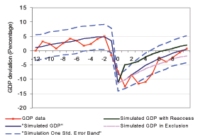
Data for Figure 4
| Quarter | GDP: Data | GDP: Simulated | Simulation One Std. Error Band: Upper | Simulation One Std. Error Band: Lower | Simulated GDP with Reaccess | Simulated GDP in Exclusion |
|---|---|---|---|---|---|---|
| -12 | 3.263 | 1.097 | 5.524 | -3.330 | - | - |
| -11 | 2.397 | 1.445 | 5.750 | -2.860 | - | - |
| -10 | 0.705 | 2.078 | 6.512 | -2.357 | - | - |
| -9 | 2.559 | 2.444 | 6.818 | -1.931 | - | - |
| -8 | 4.260 | 2.838 | 7.174 | -1.499 | - | - |
| -7 | 3.425 | 3.074 | 7.548 | -1.401 | - | - |
| -6 | 1.710 | 3.593 | 8.146 | -0.961 | - | - |
| -5 | 2.362 | 4.182 | 8.517 | -0.153 | - | - |
| -4 | 4.021 | 4.404 | 8.695 | 0.112 | - | - |
| -3 | 5.054 | 4.773 | 9.022 | 0.525 | - | - |
| -2 | -1.642 | 4.816 | 9.222 | 0.410 | - | - |
| -1 | -7.226 | 3.506 | 7.771 | -0.760 | - | - |
| 0 | -12.561 | -11.292 | -8.462 | -14.122 | -11.292 | -11.292 |
| 1 | -8.619 | -10.148 | -6.944 | -13.352 | -5.000 | -10.148 |
| 2 | -11.569 | -8.416 | -4.618 | -12.214 | -4.479 | -8.864 |
| 3 | -10.901 | -6.799 | -2.712 | -10.886 | -3.728 | -7.538 |
| 4 | -8.165 | -5.136 | -0.828 | -9.444 | -2.231 | -6.320 |
| 5 | -2.571 | -3.946 | 0.402 | -8.293 | -1.284 | -5.444 |
| 6 | -3.912 | -2.786 | 1.714 | -7.286 | -0.377 | -4.577 |
| 7 | -2.404 | -1.935 | 2.600 | -6.470 | 0.256 | -3.924 |
| 8 | -0.580 | -0.908 | 3.541 | -5.356 | 0.771 | -2.842 |
| 9 | 0.730 | -0.136 | 4.455 | -4.726 | 1.436 | -2.289 |
| 10 | 0.447 | 0.484 | 5.229 | -4.261 | 1.971 | -1.938 |
Figure 4 shows that the model produces a substantial output drop
when the country defaults, equivalent to about 13 percent of the
pre-default output level. Defaults in this baseline calibration are
always triggered by adverse productivity shocks, but these shocks
do not need to be unusually large. The standard deviation of the
calibrated TFP process (
![]() ) is 3.69 percent. By
contrast, the average decline in TFP in default events (i.e. at
) is 3.69 percent. By
contrast, the average decline in TFP in default events (i.e. at
![]() in Figure 4) is 6 percent, which is 1.6
times the standard deviation of TFP, and hence within the
two-standard-deviations range. This suggests that the model
embodies a business cycle transmission mechanism that can amplify
significantly the real effects of TFP shocks when these shocks
trigger default.
in Figure 4) is 6 percent, which is 1.6
times the standard deviation of TFP, and hence within the
two-standard-deviations range. This suggests that the model
embodies a business cycle transmission mechanism that can amplify
significantly the real effects of TFP shocks when these shocks
trigger default.
The model displays a V-shaped recovery during the financial
exclusion period. This occurs because the shock is mean-reverting,
and hence TFP is likely to improve in the periods after default
(for example, on average in the simulations TFP rises by 1 percent
at ![]() ). Therefore, even though the country
remains financially excluded on average at dates 1 to 10, the
economy recovers because TFP improves. Note that the relative
magnitudes of the recession and recovery match the data quite well.
The output dynamics for Argentina before and after the 2001 debt
crisis are mostly within the one-standard-error bands of the model
simulation.
). Therefore, even though the country
remains financially excluded on average at dates 1 to 10, the
economy recovers because TFP improves. Note that the relative
magnitudes of the recession and recovery match the data quite well.
The output dynamics for Argentina before and after the 2001 debt
crisis are mostly within the one-standard-error bands of the model
simulation.
These V-shaped dynamics are qualitatively consistent with the data of many emerging markets that suffered Sudden Stops. Calvo, Izquierdo and Talvi (2006) conducted a detailed cross-country empirical analysis of the recovery of emerging economies from Sudden Stops, and found that most recoveries are not associated with improvements in credit market access.
Further analysis of the recovery of GDP after default shows that
the recovery is driven by both the direct effect of the rise in TFP
after the "bad shock" at default and by the surge in output that
occurs when the country re-enters credit markets. This point is
illustrated in Figure 4 by the lines that show the model
simulations for the path of GDP with continued exclusion for 10
quarters after default and with immediate re-entry one period after
default. In the first scenario, the recovery reflects only the
effect of the mean reversion of the TFP shock. GDP remains below
that in the simulation average, and it is also lower than in the
data starting in the 6th quarter after default. In contrast, the
second scenario with immediate re-entry to international debt
markets shows a big rebound in GDP at ![]() because of
the efficiency gain obtained as final goods producers switch back
to imported inputs. The model simulation average lies below this
immediate re-entry line because in the model the re-entry to credit
markets is stochastic with 10 percent probability. The recovery of
GDP after default is therefore influenced by both the mean
reversion of the TFP shock and the re-entry to credit markets.
Since re-entry has a relatively low probability, however, the model
simulation for average GDP weighs more the former than the
latter.
because of
the efficiency gain obtained as final goods producers switch back
to imported inputs. The model simulation average lies below this
immediate re-entry line because in the model the re-entry to credit
markets is stochastic with 10 percent probability. The recovery of
GDP after default is therefore influenced by both the mean
reversion of the TFP shock and the re-entry to credit markets.
Since re-entry has a relatively low probability, however, the model
simulation for average GDP weighs more the former than the
latter.
The model's output dynamics also suggest that the model can
account for the seemingly dominant role of productivity shocks in
explaining output collapses during financial crises in emerging
markets. In particular, this can be the result of the efficiency
loss caused by the sectoral reallocation of labor and the fall in
use of intermediate goods when the economy defaults. To demonstrate
this point, we use the model's simulated data on aggregate factor
payments, GDP, and labor to compute Solow residuals in the standard
way: We assume an aggregate Cobb-Douglas production function for
economy-wide GDP,
![]() and compute
the Solow residual
and compute
the Solow residual ![]() using the model's data for
using the model's data for
![]() and
and ![]() , setting
, setting
![]() to the model's average of the ratio of
total wage payments to GDP,
to the model's average of the ratio of
total wage payments to GDP,
![]() , which is
about 0.7. By construction, however, the "true" TFP driving the
model is
, which is
about 0.7. By construction, however, the "true" TFP driving the
model is
![]() in the production function
of final goods.
in the production function
of final goods.
Figure 5 compares the quarter-on-quarter average growth rates of
the Solow residual, true TFP and GDP around default events in the
baseline model simulations. Clearly, there is little difference
between the Solow residual and true TFP except when the economy
defaults. In default events, however, the Solow residual
overestimates the true adverse TFP shock by a large margin (on
average, ![]() falls by nearly twice as much as
falls by nearly twice as much as
![]() when the economy defaults).
Moreover, a standard decomposition of the contributions of changes
in TFP and factors of production to changes in GDP shows that the
contribution of true TFP to the output collapse at default is about
28 percent. In contrast, the contribution of the Solow residual is
nearly 66 percent, which would suggest misleadingly that the
contribution of TFP shocks is 2.35 times larger than it actually
is. The large difference between the two is due to the fact that
the Solow residual treats the efficiency loss caused by the
sectoral reallocation of labor and the lower use of intermediate
goods as a reduction in TFP in final goods production.
when the economy defaults).
Moreover, a standard decomposition of the contributions of changes
in TFP and factors of production to changes in GDP shows that the
contribution of true TFP to the output collapse at default is about
28 percent. In contrast, the contribution of the Solow residual is
nearly 66 percent, which would suggest misleadingly that the
contribution of TFP shocks is 2.35 times larger than it actually
is. The large difference between the two is due to the fact that
the Solow residual treats the efficiency loss caused by the
sectoral reallocation of labor and the lower use of intermediate
goods as a reduction in TFP in final goods production.
Figure 5: Growth Rates of GDP, True TFP and Solow Residual around Default
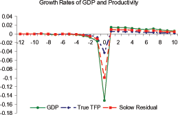
Data for Figure 5
| Quarter | GDP | Solow Residual | True TFP |
|---|---|---|---|
| -12 | -0.000300 | -0.000200 | -0.000131 |
| -11 | -0.000500 | -0.000350 | -0.000238 |
| -10 | -0.000100 | -0.000060 | -0.000041 |
| -9 | 0.001000 | 0.000700 | 0.000476 |
| -8 | -0.000900 | -0.000610 | -0.000410 |
| -7 | -0.002100 | -0.001380 | -0.000951 |
| -6 | -0.000200 | -0.000190 | -0.000131 |
| -5 | -0.000900 | -0.000590 | -0.000402 |
| -4 | -0.002100 | -0.001400 | -0.000968 |
| -3 | -0.004200 | -0.002800 | -0.001928 |
| -2 | -0.008000 | -0.005290 | -0.003626 |
| -1 | -0.016900 | -0.011310 | -0.007694 |
| 0 | -0.152000 | -0.099340 | -0.042629 |
| 1 | 0.015300 | 0.010000 | 0.005890 |
| 2 | 0.014200 | 0.009320 | 0.005422 |
| 3 | 0.014500 | 0.009460 | 0.005110 |
| 4 | 0.012800 | 0.008440 | 0.004790 |
| 5 | 0.011200 | 0.007330 | 0.003765 |
| 6 | 0.010400 | 0.006860 | 0.003289 |
| 7 | 0.011500 | 0.007510 | 0.003610 |
| 8 | 0.008800 | 0.005820 | 0.002674 |
| 9 | 0.007500 | 0.004930 | 0.002362 |
| 10 | 0.007000 | 0.004570 | 0.001821 |
Figure 6: Dynamics of Output and Sovereign Spreads before a Debt Crisis
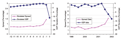
Data for Figure 6 - Panel A
| Quarter | Simulated GDP | Simulated Spread |
|---|---|---|
| -12 | 1.097 | 0.73118 |
| -11 | 1.445 | 0.73082 |
| -10 | 2.078 | 0.72132 |
| -9 | 2.444 | 0.71971 |
| -8 | 2.838 | 0.73011 |
| -7 | 3.074 | 0.76527 |
| -6 | 3.593 | 0.78649 |
| -5 | 4.182 | 0.74323 |
| -4 | 4.404 | 0.80484 |
| -3 | 4.773 | 0.82081 |
| -2 | 4.816 | 0.92933 |
| -1 | 3.506 | 1.4364 |
| 0 | -11.292 | - |
Data for Figure 6 - Panel B
| Quarter | GDP data | Spread data |
|---|---|---|
| 1999.1 | 3.2625 | 1.7675 |
| 1999.2 | 2.3970 | 1.6600 |
| 1999.3 | 0.7048 | 1.9375 |
| 1999.4 | 2.5586 | 1.6675 |
| 2000.1 | 4.2605 | 1.2875 |
| 2000.2 | 3.4247 | 1.4450 |
| 2000.3 | 1.7103 | 1.6725 |
| 2000.4 | 2.3616 | 1.7000 |
| 2001.1 | 4.0210 | 1.9325 |
| 2001.2 | 5.0537 | 2.3750 |
| 2001.3 | -1.6424 | 2.6475 |
| 2001.4 | -7.2261 | 4.1300 |
| 2002.1 | -12.5613 | - |
The model also matches nicely the dynamics of sovereign bond
spreads before a debt crisis. The left panel of Figure 6 presents
event windows showing the mean of simulated output and bond spreads
up to 12 quarters before default events in the stationary
distribution of the model. This plot clearly illustrates the
negative correlation between output and bond spreads before a debt
crisis. In particular, the spread increases as the country
approaches a debt crisis. The average quarterly spread
increases from 0.7 percent at ![]() to almost 1.5
percent in the quarter before default. At the same time, HP
detrended output starts to decline three quarters before default
and suffers a sharp drop when default occurs. These features match
relatively well the Argentine experience. The right-side panel of
Figure 6 shows the HP detrended real GDP and EMBI+ sovereign bond
spreads for Argentina from 1994Q1 to 2001 Q4. The data show a
relatively stable sovereign spread before 2000 and a sharp increase
in 2001, and Argentina also experienced a relatively steady output
performance and then a very deep recession starting in 2001. Hence,
our model seems capable of generating endogenous output and
sovereign spread dynamics consistent with the data.
to almost 1.5
percent in the quarter before default. At the same time, HP
detrended output starts to decline three quarters before default
and suffers a sharp drop when default occurs. These features match
relatively well the Argentine experience. The right-side panel of
Figure 6 shows the HP detrended real GDP and EMBI+ sovereign bond
spreads for Argentina from 1994Q1 to 2001 Q4. The data show a
relatively stable sovereign spread before 2000 and a sharp increase
in 2001, and Argentina also experienced a relatively steady output
performance and then a very deep recession starting in 2001. Hence,
our model seems capable of generating endogenous output and
sovereign spread dynamics consistent with the data.
Figure 7: Macro Dynamics around Default Episodes
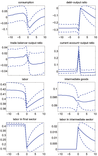
Data for Figure 7
| Quarter | consumption | consumption +one s.d. | consumption -one s.d. | debt/GDP | debt/GDP +one s.d. | debt/GDP -one s.d. | tb/GDP | tb/GDP +one s.d. | tb/GDP -one s.d. | ca/GDP | ca/GDP +one s.d. | ca/GDP -one s.d. | L | L +one s.d. | L -one s.d. | m | m +one s.d. | m -one s.d. | Lf | Lf +one s.d. | Lf -one s.d. |
|---|---|---|---|---|---|---|---|---|---|---|---|---|---|---|---|---|---|---|---|---|---|
| -12 | 0.0111 | 0.0761 | -0.0538 | -0.2776 | -0.2237 | -0.3315 | 0.0003 | 0.0289 | -0.0284 | -0.0057 | 0.0226 | -0.0340 | 0.4182 | 0.4125 | -0.4238 | 0.0961 | 0.1037 | 0.0886 | 0.4182 | 0.4338 | 0.4025 |
| -11 | 0.0128 | 0.0751 | -0.0496 | -0.2786 | -0.2243 | -0.3329 | 0.0013 | 0.0293 | -0.0267 | -0.0058 | 0.0218 | -0.0334 | 0.4180 | 0.4122 | -0.4238 | 0.0961 | 0.1036 | 0.0886 | 0.4180 | 0.4336 | 0.4025 |
| -10 | 0.0157 | 0.0779 | -0.0464 | -0.2787 | -0.2247 | -0.3326 | 0.0018 | 0.0298 | -0.0263 | -0.0065 | 0.0210 | -0.0340 | 0.4180 | 0.4115 | -0.4245 | 0.0961 | 0.1037 | 0.0885 | 0.4180 | 0.4337 | 0.4023 |
| -9 | 0.0213 | 0.0810 | -0.0384 | -0.2784 | -0.2236 | -0.3332 | 0.0012 | 0.0289 | -0.0266 | -0.0083 | 0.0190 | -0.0355 | 0.4182 | 0.4100 | -0.4265 | 0.0962 | 0.1035 | 0.0888 | 0.4182 | 0.4334 | 0.4031 |
| -8 | 0.0235 | 0.0849 | -0.0378 | -0.2793 | -0.2264 | -0.3322 | 0.0023 | 0.0303 | -0.0257 | -0.0086 | 0.0190 | -0.0361 | 0.4181 | 0.4095 | -0.4266 | 0.0961 | 0.1035 | 0.0886 | 0.4180 | 0.4334 | 0.4027 |
| -7 | 0.0235 | 0.0839 | -0.0370 | -0.2801 | -0.2262 | -0.3340 | 0.0049 | 0.0332 | -0.0234 | -0.0073 | 0.0207 | -0.0354 | 0.4176 | 0.4103 | -0.4250 | 0.0959 | 0.1031 | 0.0886 | 0.4176 | 0.4326 | 0.4026 |
| -6 | 0.0292 | 0.0902 | -0.0318 | -0.2783 | -0.2261 | -0.3305 | 0.0039 | 0.0317 | -0.0240 | -0.0097 | 0.0179 | -0.0372 | 0.4176 | 0.4079 | -0.4272 | 0.0958 | 0.1030 | 0.0887 | 0.4176 | 0.4324 | 0.4027 |
| -5 | 0.0328 | 0.0949 | -0.0293 | -0.2781 | -0.2262 | -0.3301 | 0.0047 | 0.0328 | -0.0235 | -0.0103 | 0.0176 | -0.0383 | 0.4174 | 0.4071 | -0.4277 | 0.0958 | 0.1029 | 0.0886 | 0.4174 | 0.4321 | 0.4026 |
| -4 | 0.0343 | 0.0939 | -0.0253 | -0.2783 | -0.2267 | -0.3298 | 0.0065 | 0.0337 | -0.0208 | -0.0098 | 0.0175 | -0.0370 | 0.4170 | 0.4072 | -0.4267 | 0.0955 | 0.1026 | 0.0885 | 0.4170 | 0.4315 | 0.4024 |
| -3 | 0.0330 | 0.0939 | -0.0279 | -0.2778 | -0.2266 | -0.3291 | 0.0091 | 0.0373 | -0.0192 | -0.0085 | 0.0199 | -0.0368 | 0.4161 | 0.4077 | -0.4246 | 0.0951 | 0.1021 | 0.0881 | 0.4161 | 0.4306 | 0.4016 |
| -2 | 0.0275 | 0.0870 | -0.0319 | -0.2768 | -0.2256 | -0.3279 | 0.0121 | 0.0396 | -0.0153 | -0.0067 | 0.0209 | -0.0344 | 0.4145 | 0.4078 | -0.4213 | 0.0944 | 0.1012 | 0.0875 | 0.4145 | 0.4287 | 0.4004 |
| -1 | 0.0095 | 0.0676 | -0.0485 | -0.2762 | -0.2251 | -0.3274 | 0.0184 | 0.0448 | -0.0080 | -0.0023 | 0.0243 | -0.0289 | 0.4112 | 0.4089 | -0.4135 | 0.0927 | 0.0992 | 0.0863 | 0.4112 | 0.4247 | 0.3977 |
| 0 | -0.0708 | -0.0388 | -0.1028 | -0.3116 | -0.2471 | -0.3760 | 0.0031 | 0.0089 | -0.0027 | 0.2999 | 0.3631 | 0.2366 | 0.3813 | 0.6811 | -0.0814 | 0.0931 | 0.0944 | 0.0919 | 0.1612 | 0.1643 | 0.1581 |
| 1 | -0.0919 | -0.0346 | -0.1492 | 0.0000 | 0.0000 | 0.0000 | -0.0077 | 0.0265 | -0.0419 | -0.0226 | 0.0117 | -0.0569 | 0.3842 | 0.3616 | -0.4068 | 0.0926 | 0.0958 | 0.0894 | 0.1854 | 0.2558 | 0.1151 |
| 2 | -0.0706 | -0.0085 | -0.1327 | -0.0118 | 0.0238 | -0.0474 | -0.0112 | 0.0243 | -0.0467 | -0.0259 | 0.0101 | -0.0619 | 0.3869 | 0.3610 | -0.4128 | 0.0923 | 0.0964 | 0.0881 | 0.2068 | 0.2987 | 0.1149 |
| 3 | -0.0524 | 0.0119 | -0.1168 | -0.0281 | 0.0327 | -0.0889 | -0.0121 | 0.0247 | -0.0489 | -0.0265 | 0.0107 | -0.0637 | 0.3897 | 0.3633 | -0.4162 | 0.0921 | 0.0967 | 0.0875 | 0.2284 | 0.3341 | 0.1226 |
| 4 | -0.0394 | 0.0273 | -0.1061 | -0.0463 | 0.0326 | -0.1252 | -0.0101 | 0.0247 | -0.0449 | -0.0235 | 0.0126 | -0.0596 | 0.3922 | 0.3687 | -0.4157 | 0.0922 | 0.0971 | 0.0874 | 0.2441 | 0.3570 | 0.1312 |
| 5 | -0.0287 | 0.0402 | -0.0976 | -0.0631 | 0.0300 | -0.1562 | -0.0085 | 0.0266 | -0.0435 | -0.0212 | 0.0149 | -0.0573 | 0.3944 | 0.3732 | -0.4156 | 0.0923 | 0.0974 | 0.0872 | 0.2593 | 0.3769 | 0.1417 |
| 6 | -0.0183 | 0.0499 | -0.0865 | -0.0792 | 0.0244 | -0.1828 | -0.0080 | 0.0270 | -0.0430 | -0.0194 | 0.0188 | -0.0575 | 0.3965 | 0.3771 | -0.4159 | 0.0925 | 0.0977 | 0.0873 | 0.2735 | 0.3939 | 0.1531 |
| 7 | -0.0081 | 0.0596 | -0.0759 | -0.0949 | 0.0162 | -0.2061 | -0.0072 | 0.0289 | -0.0434 | -0.0181 | 0.0191 | -0.0553 | 0.3987 | 0.3806 | -0.4169 | 0.0928 | 0.0982 | 0.0873 | 0.2883 | 0.4100 | 0.1665 |
| 8 | -0.0022 | 0.0672 | -0.0716 | -0.1111 | 0.0055 | -0.2276 | -0.0053 | 0.0299 | -0.0405 | -0.0153 | 0.0213 | -0.0518 | 0.4005 | 0.3852 | -0.4158 | 0.0930 | 0.0987 | 0.0873 | 0.3000 | 0.4217 | 0.1782 |
| 9 | 0.0007 | 0.0691 | -0.0677 | -0.1262 | -0.0049 | -0.2474 | -0.0023 | 0.0322 | -0.0367 | -0.0107 | 0.0271 | -0.0485 | 0.4020 | 0.3912 | -0.4127 | 0.0932 | 0.0990 | 0.0873 | 0.3096 | 0.4304 | 0.1887 |
| 10 | 0.0051 | 0.0715 | -0.0612 | -0.1379 | -0.0144 | -0.2614 | -0.0020 | 0.0324 | -0.0364 | -0.0099 | 0.0259 | -0.0457 | 0.4034 | 0.3935 | -0.4133 | 0.0934 | 0.0993 | 0.0875 | 0.3197 | 0.4388 | 0.2007 |
Figure 7 shows the event windows for the average of the model
simulations of consumption, the GDP ratios of the trade balance,
current account and debt, as well as labor, intermediate goods, and
sectoral labor allocations (along with the corresponding
one-standard-error bands). Consumption drops sharply when the
government defaults and in the period that follows, and then it
recovers following the V-shaped dynamics of GDP. The debt-output
ratio is over 26 percent on average before default, and it
increases to about 32 percent in the period just before default.
The external accounts also experience sharp adjustments around
default episodes. In particular, the model generates a sharp
reversal in the current account. The country runs a small current
account deficit on average, but default, and the loss of credit
market access that it entails, produce a large jump of about 30
percentage points of GDP in the current account. Labor and the
allocation of intermediate goods also fall sharply when the economy
defaults. Moreover, since default triggers a shift from imported to
domestic inputs in final goods production, labor is reallocated
from the ![]() sector to the
sector to the ![]() sector.
sector.
The sharp declines in GDP, consumption, labor and intermediate goods, together with the large reversal in the current account, indicate that the model yields predictions consistent with the sudden stop phenomenon observed in emerging economies around financial crises. In most of the sudden stops literature, however, the current account reversal is modeled as an exogenous shock, whereas in this model both the current account reversal and the economic collapse are endogenous. Moreover, this endogenous sudden stop is driven by default risk determined by an optimal recursive contract, instead of the ad-hoc collateral constraints emphasized in other models of endogenous sudden stops (see Mendoza (2007)).
3.4 Key Features of the Equilibrium with Default
How does the interaction between endogenous output fluctuations and endogenous default risk affect the quantitative performance of the model? We answer this question by studying the behavior of the value function when the country has access to world financial markets, the sovereign bond pricing function, the saving decision rule, and output. Figure 8 shows these equilibrium functions for high and low TFP shocks as a function of the country's foreign asset position.
The first panel of Figure 8 shows that the value function
increases with the asset position for the range of asset positions
higher than the value at which default is certain (for asset
positions smaller than this value, the value function becomes
independent of foreign assets). As the country's debt increases
(i.e. assets fall) the value of default can exceed the value of not
defaulting. The country is more likely to default if TFP is low
because the default option is more attractive. This is because it
is more painful to repay the debt in a bad state, while at the same
time default does not lead to a high output loss compared to the
case with a good TFP shock. The value function also differs as we
vary the amount of working capital ![]() . The
value of default increases with working capital because the
government transfers the repayment of working capital loans to
households when it defaults.
. The
value of default increases with working capital because the
government transfers the repayment of working capital loans to
households when it defaults.
The second panel of Figure 8 shows that sovereign bond prices increase with asset holdings (i.e. decrease with the debt position), reflecting the standard result that default risk premia are higher at higher levels of debt. Moreover, bond prices are higher when the country experiences a good TFP shock, and higher bond prices imply lower default risk premia, lower default probabilities and lower country interest rates. Working capital financing becomes less costly as a result, leading final goods producers to increase demand for foreign inputs and produce more. This feedback from country interest rates to output dynamics also affects the country's incentives to default, reinforcing the reduction in default risk. The opposite is true when the country experiences a bad TFP shock, and this is an important result because it implies that, for any given level of debt before the country is in financial autarky, default is more likely when TFP is low than when it is high (recall that the TFP shock and asset position are the only state variables that determine bond prices in the model).
Figure 8: Value Function and Decision Rules
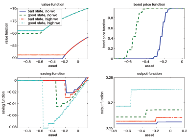
Data for Figure 8
Asset | Value (bad state, no wc) | Value (good state, no wc) | Value (bad state, high wc) | Value (good state, high wc) | Bond price (bad state) | Bond price (good state) | Saving (bad state, no wc) | Saving (good state, no wc) | Saving (bad state, high wc) | Saving (good state, high wc) | Output (bad state, no wc) | Output (good state, no wc) | Output (bad state, high wc) | Output (good state, high wc) |
|---|---|---|---|---|---|---|---|---|---|---|---|---|---|---|
| -0.9184 | -50.6743 | -45.5789 | -50.0075 | -45.0780 | - | - | - | - | - | - | - | - | - | - |
| -0.9056 | -50.6743 | -45.5789 | -50.0075 | -45.0780 | - | - | - | - | - | - | - | - | - | - |
| -0.8929 | -50.6743 | -45.5789 | -50.0075 | -45.0780 | - | - | - | - | - | - | - | - | - | - |
| -0.8801 | -50.6743 | -45.5789 | -50.0075 | -45.0780 | - | - | - | - | - | - | - | - | - | - |
| -0.8674 | -50.6743 | -45.5789 | -50.0075 | -45.0780 | - | - | - | - | - | - | - | - | - | - |
| -0.8546 | -50.6743 | -45.5789 | -50.0075 | -45.0780 | - | - | - | - | - | - | - | - | - | - |
| -0.8418 | -50.6743 | -45.5789 | -50.0075 | -45.0780 | - | - | - | - | - | - | - | - | - | - |
| -0.8291 | -50.6743 | -45.5789 | -50.0075 | -45.0780 | - | - | - | - | - | - | - | - | - | - |
| -0.8163 | -50.6743 | -45.5789 | -50.0075 | -45.0780 | - | - | - | - | - | - | - | - | - | - |
| -0.8036 | -50.6743 | -45.5789 | -50.0075 | -45.0780 | - | - | - | - | - | - | - | - | - | - |
| -0.7908 | -50.6743 | -45.5789 | -50.0075 | -45.0780 | - | - | - | - | - | - | - | - | - | - |
| -0.7781 | -50.6743 | -45.5789 | -50.0075 | -45.0780 | - | - | - | - | - | - | - | - | - | - |
| -0.7653 | -50.6743 | -45.5789 | -50.0075 | -45.0780 | - | - | - | - | - | - | - | - | - | - |
| -0.7526 | -50.6743 | -45.5789 | -50.0075 | -45.0780 | - | - | - | - | - | - | - | - | - | - |
| -0.7398 | -50.6743 | -45.5789 | -50.0075 | -45.0780 | 0.0000 | 0.0001 | 0.0000 | 0.0000 | 0.0000 | 0.0000 | 0.1883 | 0.2185 | 0.1883 | 0.2185 |
| -0.7270 | -50.6743 | -45.5789 | -50.0075 | -45.0780 | 0.0000 | 0.0001 | 0.0000 | 0.0000 | 0.0000 | 0.0000 | 0.1883 | 0.2185 | 0.1883 | 0.2185 |
| -0.7143 | -50.6743 | -45.5789 | -50.0075 | -45.0780 | 0.0000 | 0.0001 | 0.0000 | 0.0000 | 0.0000 | 0.0000 | 0.1883 | 0.2185 | 0.1883 | 0.2185 |
| -0.7015 | -50.6743 | -45.5789 | -50.0075 | -45.0780 | 0.0000 | 0.0014 | 0.0000 | 0.0000 | 0.0000 | 0.0000 | 0.1883 | 0.2185 | 0.1883 | 0.2185 |
| -0.6888 | -50.6743 | -45.5789 | -50.0075 | -45.0780 | 0.0000 | 0.0014 | 0.0000 | 0.0000 | 0.0000 | 0.0000 | 0.1883 | 0.2185 | 0.1883 | 0.2185 |
| -0.6760 | -50.6743 | -45.5789 | -50.0075 | -45.0780 | 0.0000 | 0.0014 | 0.0000 | 0.0000 | 0.0000 | 0.0000 | 0.1883 | 0.2185 | 0.1883 | 0.2185 |
| -0.6633 | -50.6743 | -45.5789 | -50.0075 | -45.0780 | 0.0000 | 0.0014 | 0.0000 | 0.0000 | 0.0000 | 0.0000 | 0.1883 | 0.2185 | 0.1883 | 0.2185 |
| -0.6505 | -50.6743 | -45.5789 | -50.0075 | -45.0780 | 0.0000 | 0.0132 | 0.0000 | 0.0000 | 0.0000 | 0.0000 | 0.1883 | 0.2185 | 0.1883 | 0.2185 |
| -0.6378 | -50.6743 | -45.5789 | -50.0075 | -45.0780 | 0.0000 | 0.0132 | 0.0000 | 0.0000 | 0.0000 | 0.0000 | 0.1883 | 0.2185 | 0.1883 | 0.2185 |
| -0.6250 | -50.6743 | -45.5789 | -50.0075 | -45.0780 | 0.0000 | 0.0132 | 0.0000 | 0.0000 | 0.0000 | 0.0000 | 0.1883 | 0.2185 | 0.1883 | 0.2185 |
| -0.6123 | -50.6743 | -45.5789 | -50.0075 | -45.0780 | 0.0000 | 0.0724 | 0.0000 | 0.0000 | 0.0000 | 0.0000 | 0.1883 | 0.2185 | 0.1883 | 0.2185 |
| -0.5995 | -50.6743 | -45.5789 | -50.0075 | -45.0780 | 0.0000 | 0.0724 | 0.0000 | 0.0000 | 0.0000 | 0.0000 | 0.1883 | 0.2185 | 0.1883 | 0.2185 |
| -0.5867 | -50.6743 | -45.5789 | -50.0075 | -45.0780 | 0.0000 | 0.0724 | 0.0000 | 0.0000 | 0.0000 | 0.0000 | 0.1883 | 0.2185 | 0.1883 | 0.2185 |
| -0.5740 | -50.6743 | -45.5789 | -50.0075 | -45.0780 | 0.0000 | 0.0724 | 0.0000 | 0.0000 | 0.0000 | 0.0000 | 0.1883 | 0.2185 | 0.1883 | 0.2185 |
| -0.5612 | -50.6743 | -45.4879 | -50.0075 | -45.0780 | 0.0000 | 0.2432 | 0.0000 | -0.0911 | 0.0000 | 0.0000 | 0.1883 | 0.2489 | 0.1883 | 0.2185 |
| -0.5485 | -50.6743 | -45.3189 | -50.0075 | -45.0780 | 0.0000 | 0.2432 | 0.0000 | -0.0911 | 0.0000 | 0.0000 | 0.1883 | 0.2489 | 0.1883 | 0.2185 |
| -0.5357 | -50.6743 | -45.1571 | -50.0075 | -45.0780 | 0.0000 | 0.2432 | 0.0000 | -0.0911 | 0.0000 | 0.0000 | 0.1883 | 0.2489 | 0.1883 | 0.2185 |
| -0.5230 | -50.6743 | -45.0021 | -50.0075 | -45.0021 | 0.0000 | 0.5252 | 0.0000 | -0.0911 | 0.0000 | -0.0911 | 0.1883 | 0.2489 | 0.1883 | 0.2489 |
| -0.5102 | -50.6743 | -44.8533 | -50.0075 | -44.8533 | 0.0000 | 0.5252 | 0.0000 | -0.0911 | 0.0000 | -0.0911 | 0.1883 | 0.2489 | 0.1883 | 0.2489 |
| -0.4975 | -50.6743 | -44.7105 | -50.0075 | -44.7105 | 0.0000 | 0.5252 | 0.0000 | -0.0911 | 0.0000 | -0.0911 | 0.1883 | 0.2489 | 0.1883 | 0.2489 |
| -0.4847 | -50.6743 | -44.5733 | -50.0075 | -44.5733 | 0.0000 | 0.7920 | 0.0000 | -0.0911 | 0.0000 | -0.0911 | 0.1883 | 0.2489 | 0.1883 | 0.2489 |
| -0.4719 | -50.6743 | -44.4413 | -50.0075 | -44.4413 | 0.0000 | 0.7920 | 0.0000 | -0.0911 | 0.0000 | -0.0911 | 0.1883 | 0.2489 | 0.1883 | 0.2489 |
| -0.4592 | -50.6743 | -44.3144 | -50.0075 | -44.3144 | 0.0000 | 0.7920 | 0.0000 | -0.0911 | 0.0000 | -0.0911 | 0.1883 | 0.2489 | 0.1883 | 0.2489 |
| -0.4464 | -50.6743 | -44.1921 | -50.0075 | -44.1921 | 0.0000 | 0.9365 | 0.0000 | -0.0911 | 0.0000 | -0.0911 | 0.1883 | 0.2489 | 0.1883 | 0.2489 |
| -0.4337 | -50.6743 | -44.0742 | -50.0075 | -44.0742 | 0.0000 | 0.9365 | 0.0000 | -0.0911 | 0.0000 | -0.0911 | 0.1883 | 0.2489 | 0.1883 | 0.2489 |
| -0.4209 | -50.6743 | -43.9606 | -50.0075 | -43.9606 | 0.0008 | 0.9365 | 0.0000 | -0.0911 | 0.0000 | -0.0911 | 0.1883 | 0.2489 | 0.1883 | 0.2489 |
| -0.4082 | -50.6743 | -43.8509 | -50.0075 | -43.8509 | 0.0008 | 0.9813 | 0.0000 | -0.0911 | 0.0000 | -0.0911 | 0.1883 | 0.2489 | 0.1883 | 0.2489 |
| -0.3954 | -50.6743 | -43.7451 | -50.0075 | -43.7451 | 0.0008 | 0.9813 | 0.0000 | -0.0911 | 0.0000 | -0.0911 | 0.1883 | 0.2489 | 0.1883 | 0.2489 |
| -0.3827 | -50.6743 | -43.6359 | -50.0075 | -43.6359 | 0.0088 | 0.9813 | 0.0000 | -0.0826 | 0.0000 | -0.0826 | 0.1883 | 0.2491 | 0.1883 | 0.2491 |
| -0.3699 | -50.6743 | -43.5275 | -50.0075 | -43.5275 | 0.0088 | 0.9892 | 0.0000 | -0.0826 | 0.0000 | -0.0826 | 0.1883 | 0.2491 | 0.1883 | 0.2491 |
| -0.3571 | -50.6743 | -43.4228 | -50.0075 | -43.4228 | 0.0088 | 0.9892 | 0.0000 | -0.0826 | 0.0000 | -0.0826 | 0.1883 | 0.2491 | 0.1883 | 0.2491 |
| -0.3444 | -50.6743 | -43.3216 | -50.0075 | -43.3216 | 0.0536 | 0.9901 | 0.0000 | -0.0826 | 0.0000 | -0.0826 | 0.1883 | 0.2491 | 0.1883 | 0.2491 |
| -0.3316 | -50.6743 | -43.2237 | -50.0075 | -43.2237 | 0.0536 | 0.9901 | 0.0000 | -0.0826 | 0.0000 | -0.0826 | 0.1883 | 0.2491 | 0.1883 | 0.2491 |
| -0.3189 | -50.6743 | -43.1291 | -50.0075 | -43.1291 | 0.0536 | 0.9901 | 0.0000 | -0.0826 | 0.0000 | -0.0826 | 0.1883 | 0.2491 | 0.1883 | 0.2491 |
| -0.3061 | -50.6743 | -43.0355 | -50.0075 | -43.0355 | 0.1981 | 0.9901 | 0.0000 | -0.0797 | 0.0000 | -0.0797 | 0.1883 | 0.2491 | 0.1883 | 0.2491 |
| -0.2934 | -50.6743 | -42.9413 | -50.0075 | -42.9413 | 0.1981 | 0.9901 | 0.0000 | -0.0769 | 0.0000 | -0.0769 | 0.1883 | 0.2491 | 0.1883 | 0.2491 |
| -0.2806 | -50.5768 | -42.8498 | -50.0075 | -42.8498 | 0.4649 | 0.9901 | -0.0427 | -0.0769 | 0.0000 | -0.0769 | 0.2011 | 0.2491 | 0.1883 | 0.2491 |
| -0.2679 | -50.3545 | -42.7604 | -50.0075 | -42.7604 | 0.4649 | 0.9901 | -0.0427 | -0.0740 | 0.0000 | -0.0740 | 0.2011 | 0.2491 | 0.1883 | 0.2491 |
| -0.2551 | -50.1431 | -42.6718 | -50.0075 | -42.6718 | 0.7469 | 0.9901 | -0.0427 | -0.0740 | 0.0000 | -0.0740 | 0.2011 | 0.2491 | 0.1883 | 0.2491 |
| -0.2423 | -49.9416 | -42.5850 | -49.9416 | -42.5850 | 0.7469 | 0.9901 | -0.0427 | -0.0712 | -0.0427 | -0.0712 | 0.2011 | 0.2491 | 0.2011 | 0.2491 |
| -0.2296 | -49.7494 | -42.4992 | -49.7494 | -42.4992 | 0.7469 | 0.9901 | -0.0427 | -0.0712 | -0.0427 | -0.0712 | 0.2011 | 0.2491 | 0.2011 | 0.2491 |
| -0.2168 | -49.5659 | -42.4146 | -49.5659 | -42.4146 | 0.9177 | 0.9901 | -0.0427 | -0.0683 | -0.0427 | -0.0683 | 0.2011 | 0.2491 | 0.2011 | 0.2491 |
| -0.2041 | -49.3906 | -42.3312 | -49.3906 | -42.3312 | 0.9177 | 0.9901 | -0.0427 | -0.0655 | -0.0427 | -0.0655 | 0.2011 | 0.2491 | 0.2011 | 0.2491 |
| -0.1913 | -49.2228 | -42.2481 | -49.2228 | -42.2481 | 0.9769 | 0.9901 | -0.0427 | -0.0655 | -0.0427 | -0.0655 | 0.2011 | 0.2491 | 0.2011 | 0.2491 |
| -0.1786 | -49.0621 | -42.1658 | -49.0621 | -42.1658 | 0.9769 | 0.9901 | -0.0427 | -0.0626 | -0.0427 | -0.0626 | 0.2011 | 0.2491 | 0.2011 | 0.2491 |
| -0.1658 | -48.9081 | -42.0852 | -48.9081 | -42.0852 | 0.9887 | 0.9901 | -0.0427 | -0.0626 | -0.0427 | -0.0626 | 0.2011 | 0.2491 | 0.2011 | 0.2491 |
| -0.1531 | -48.7603 | -42.0047 | -48.7603 | -42.0047 | 0.9887 | 0.9901 | -0.0427 | -0.0598 | -0.0427 | -0.0598 | 0.2011 | 0.2491 | 0.2011 | 0.2491 |
| -0.1403 | -48.6104 | -41.9256 | -48.6104 | -41.9256 | 0.9900 | 0.9901 | -0.0370 | -0.0569 | -0.0370 | -0.0569 | 0.2012 | 0.2491 | 0.2012 | 0.2491 |
| -0.1276 | -48.4640 | -41.8474 | -48.4640 | -41.8474 | 0.9900 | 0.9901 | -0.0370 | -0.0569 | -0.0370 | -0.0569 | 0.2012 | 0.2491 | 0.2012 | 0.2491 |
| -0.1148 | -48.3235 | -41.7696 | -48.3235 | -41.7696 | 0.9901 | 0.9901 | -0.0370 | -0.0541 | -0.0370 | -0.0541 | 0.2012 | 0.2491 | 0.2012 | 0.2491 |
| -0.1020 | -48.1884 | -41.6928 | -48.1884 | -41.6928 | 0.9901 | 0.9901 | -0.0370 | -0.0512 | -0.0370 | -0.0512 | 0.2012 | 0.2491 | 0.2012 | 0.2491 |
| -0.0893 | -48.0584 | -41.6170 | -48.0584 | -41.6170 | 0.9901 | 0.9901 | -0.0370 | -0.0512 | -0.0370 | -0.0512 | 0.2012 | 0.2491 | 0.2012 | 0.2491 |
| -0.0765 | -47.9317 | -41.5416 | -47.9317 | -41.5416 | 0.9901 | 0.9901 | -0.0342 | -0.0484 | -0.0342 | -0.0484 | 0.2012 | 0.2491 | 0.2012 | 0.2491 |
| -0.0638 | -47.8054 | -41.4669 | -47.8054 | -41.4669 | 0.9901 | 0.9901 | -0.0313 | -0.0456 | -0.0313 | -0.0456 | 0.2013 | 0.2491 | 0.2013 | 0.2491 |
| -0.0510 | -47.6805 | -41.3931 | -47.6805 | -41.3931 | 0.9901 | 0.9901 | -0.0313 | -0.0427 | -0.0313 | -0.0427 | 0.2013 | 0.2491 | 0.2013 | 0.2491 |
| -0.0383 | -47.5601 | -41.3195 | -47.5601 | -41.3195 | 0.9901 | 0.9901 | -0.0285 | -0.0427 | -0.0285 | -0.0427 | 0.2013 | 0.2491 | 0.2013 | 0.2491 |
| -0.0255 | -47.4398 | -41.2466 | -47.4398 | -41.2466 | 0.9901 | 0.9901 | -0.0285 | -0.0399 | -0.0285 | -0.0399 | 0.2013 | 0.2491 | 0.2013 | 0.2491 |
| -0.0128 | -47.3235 | -41.1746 | -47.3235 | -41.1746 | 0.9901 | 0.9901 | -0.0256 | -0.0370 | -0.0256 | -0.0370 | 0.2013 | 0.2491 | 0.2013 | 0.2491 |
| 0.0000 | -47.2076 | -41.1031 | -47.2076 | -41.1031 | 0.9901 | 0.9901 | -0.0256 | -0.0370 | -0.0256 | -0.0370 | 0.2013 | 0.2491 | 0.2013 | 0.2491 |
| 0.0224 | -47.0093 | -40.9789 | -47.0093 | -40.9789 | 0.9901 | 0.9901 | -0.0228 | -0.0313 | -0.0228 | -0.0313 | 0.2013 | 0.2491 | 0.2013 | 0.2491 |
| 0.0448 | -46.8151 | -40.8564 | -46.8151 | -40.8564 | 0.9901 | 0.9901 | -0.0199 | -0.0285 | -0.0199 | -0.0285 | 0.2013 | 0.2491 | 0.2013 | 0.2491 |
The lower-left panel of Figure 8 shows that the country borrows less (i.e. chooses a higher asset position) when it experiences a low TFP shock. This property of the assets decision rule is reflected in the countercyclical trade balance and the positive correlation between the trade balance and sovereign spreads documented earlier.
Finally, the lower-right panel of Figure 8 shows that the relationship between output and foreign assets follows "almost" a two-step function. The lower step corresponds to the range of high debt in which firms operate with domestic inputs, either because the country defaults or because the interest rate is sufficiently high and the state of productivity is sufficiently low. The higher step pertains to the range of debt positions when the country has access to world credit markets and firms use imported inputs. Output in this region depends on the asset position (so the output plots are not truly two step functions), but the Figure would need a finer scale for the relationship to be visible. In this region, output fluctuates with country risk because the demand for imported intermediate goods is directly affected by country spreads. When the country borrows more, default risk increases and this raises the financing cost of working capital to firms. In response, firms cut demand for imported inputs and output falls. The plot also shows that the size of the output drop at default is larger with the good productivity shock because the cost of default is increasing in TFP, as explained earlier.
4 Sensitivity Analysis
4.1 Working capital
The working capital constraint plays an important role in the
quantitative performance of the model. Its relevance can be
illustrated by comparing the benchmark results with the results of
a simulation that abstracts from working capital (i.e., ![]() ). Without working capital, the output loss at
default is invariant to changes in productivity, as in the existing
quantitative studies of sovereign debt that assume that income is
an exogenous endowment (e.g. Aguiar and Gopinath (2006), Yue
(2006)). To keep the results comparable, we introduce an exogenous
output loss at default in this variant of our model and calibrate
it so as to keep matching the average output loss in default of 13
percent observed in the data, which we used as a calibration target
in the benchmark calibration. The other parameters are kept
unchanged. The second column of Table 4 presents the simulation
results for this no-working-capital case and the third column
reproduces the results for the benchmark model.
). Without working capital, the output loss at
default is invariant to changes in productivity, as in the existing
quantitative studies of sovereign debt that assume that income is
an exogenous endowment (e.g. Aguiar and Gopinath (2006), Yue
(2006)). To keep the results comparable, we introduce an exogenous
output loss at default in this variant of our model and calibrate
it so as to keep matching the average output loss in default of 13
percent observed in the data, which we used as a calibration target
in the benchmark calibration. The other parameters are kept
unchanged. The second column of Table 4 presents the simulation
results for this no-working-capital case and the third column
reproduces the results for the benchmark model.
Table 4: Changes in the Working Capital Constraint
| Statistics | No WC | Benchmark θ = 0.1 | Larger WC θ = 0.2 | Larger WC θ = 0.3 |
|---|---|---|---|---|
| Output loss | 12.5% | 13.0% | 12.8% | 11.7% |
| GDP std. dev. | 4.64% | 4.72% | 4.98% | 5.00% |
| Default probability | 0.04% | 0.69% | 0.81% | 0.82% |
| Corr. between Spreads and GDP | -0.10 | -0.48 | -0.52 | -0.45 |
| Corr. between Spreads and TB | -0.26 | 0.39 | 0.36 | 0.39 |
| Corr. between TB and GDP | -0.28 | -0.42 | -0.39 | -0.41 |
| Debt/GDP | 6.91% | 26.05% | 15.79% | 9.59% |
| Bond spreads std. dev. | 0.07% | 0.71% | 0.76% | 0.73% |
| Average Bond Spreads | 0.04% | 0.69% | 0.81% | 0.82% |
| Trade Balance std. dev. | 1.80% | 2.88% | 2.68% | 2.18% |
The model without working capital performs much worse in terms of its ability to match all of the important features of the data that the benchmark model mimicked well. The frequency of defaults falls from 0.7 percent to 0.04 percent. The GDP correlations of sovereign spreads and net exports increase sharply. The correlation between spreads and net exports changes from significantly positive at 0.39 to negative at -0.26. The mean debt ratio declines by nearly 20 percentage points of GDP, and the average and standard deviation of country spreads fall by about 70 basis points. These results follow from two important differences in the model without working capital relative to our setup: First, the cost of default becomes independent of the state of nature, and second, bond spreads no longer have a direct impact on production. As a result, debt is not as good a hedging mechanism as in the benchmark model with working capital, making default more painful ex ante in the model without working capital, and thus reducing the average debt ratio. Moreover, the model without working capital cannot reproduce the V-shaped output dynamics that the benchmark model produces (see Figure 4), because it maintains the disconnect between country risk and business cycles.
We have established that removing working capital worsens
significantly the quantitative performance of the model. But how
sensitive are the results to the value of the working capital
requirement beyond the extreme case of ![]() ? To
answer this question, we solved the model for
? To
answer this question, we solved the model for
![]() and
and ![]() instead of
instead of
![]() as in the benchmark case. The last two
columns of Table 4 show the results for these simulations. The
higher working capital requirement reduces sharply the mean debt
ratio, despite very small reductions in the size of the output loss
at default. In contrast, the variability of GDP, the probability of
default, and the mean and standard deviation of spreads all
increase as
as in the benchmark case. The last two
columns of Table 4 show the results for these simulations. The
higher working capital requirement reduces sharply the mean debt
ratio, despite very small reductions in the size of the output loss
at default. In contrast, the variability of GDP, the probability of
default, and the mean and standard deviation of spreads all
increase as ![]() rises.
rises.
These changes reflect the fact that the higher ![]() has opposing effects on default incentives and
production plans. On one hand, final goods producers are more
likely to switch to domestic inputs, since higher
has opposing effects on default incentives and
production plans. On one hand, final goods producers are more
likely to switch to domestic inputs, since higher ![]() increases the effective price of imported inputs, and
changes in sovereign interest rates have a larger impact on
production. These effects amplify the response of output to
productivity shocks, making output more volatile. This result is
complementary to the finding in Uribe and Yue (2006) showing that
the impact of output on country interest rates magnifies business
cycle volatility, and the result in Neumeyer and Perri (2005)
showing that working capital loans that charge sovereign interest
rates also amplify business cycle volatility. On the other hand,
default leads to a lower fraction of output loss at default on
average because the TFP shock that triggers default is smaller than
in the benchmark case with a lower
increases the effective price of imported inputs, and
changes in sovereign interest rates have a larger impact on
production. These effects amplify the response of output to
productivity shocks, making output more volatile. This result is
complementary to the finding in Uribe and Yue (2006) showing that
the impact of output on country interest rates magnifies business
cycle volatility, and the result in Neumeyer and Perri (2005)
showing that working capital loans that charge sovereign interest
rates also amplify business cycle volatility. On the other hand,
default leads to a lower fraction of output loss at default on
average because the TFP shock that triggers default is smaller than
in the benchmark case with a lower ![]() . Thus,
the output levels before and after default are closer, generating a
smaller output loss. At the same time, this lower output cost of
default and a higher volatility in GDP make the sovereign exercise
the default option more often, increasing the default probability
and the volatility of bond spreads, and reducing the mean debt/GDP
ratio. The overall quantitative effects of tightening the working
capital constraint on the debt/GDP ratio and the default frequency
are particularly large, and we get these results even though
average sovereign spreads, and hence the average interest rate on
working capital, do not deviate sharply from the one-percent risk
free rate. 16
. Thus,
the output levels before and after default are closer, generating a
smaller output loss. At the same time, this lower output cost of
default and a higher volatility in GDP make the sovereign exercise
the default option more often, increasing the default probability
and the volatility of bond spreads, and reducing the mean debt/GDP
ratio. The overall quantitative effects of tightening the working
capital constraint on the debt/GDP ratio and the default frequency
are particularly large, and we get these results even though
average sovereign spreads, and hence the average interest rate on
working capital, do not deviate sharply from the one-percent risk
free rate. 16
4.2 Costly Labor Reallocation
As we explained earlier, the shift from imported to domestic
inputs that occurs when the economy defaults reduces production
efficiency because of the costly reallocation of labor away from
final goods production. Hence, our results are likely to be
sensitive to changes in the sectoral elasticity of labor, as
determined by ![]() , because changes in this elasticity
alter the size of the efficiency loss associated with default.
, because changes in this elasticity
alter the size of the efficiency loss associated with default.
Table 5: Changes in Sectoral Labor Elasticity
| Statistics | Lower Elasticity ν = 0.39 | Benchmark ν = 0.41 | Higher Elasticity ν = 0.43 |
|---|---|---|---|
| Output loss | 16.1% | 13.0% | 11.6% |
| GDP std. dev. | 4.71% | 4.72% | 4.58% |
| Default probability | 0.34% | 0.69% | 0.92% |
| Corr. between Spreads and GDP | -0.46 | -0.48 | -0.35 |
| Corr. between Spreads and TB | 0.39 | 0.39 | 0.37 |
| Corr. between TB and GDP | -0.44 | -0.42 | -0.43 |
| Debt/GDP | 42.23% | 26.05% | 9.26% |
| Bond spreads std. dev. | 0.35% | 0.71% | 2.78% |
| Average Bond Spreads | 0.34% | 0.69% | 0.92% |
Table 5 presents simulation results comparing the benchmark case
(![]() , with an elasticity of substitution
between
, with an elasticity of substitution
between ![]() and
and ![]() of -1.7) with
cases in which
of -1.7) with
cases in which ![]() (a lower elasticity at
-1.64) and
(a lower elasticity at
-1.64) and ![]() (a higher elasticity at -1.75).
All of the other parameters are the same as in the benchmark
calibration. The results show that the value of
(a higher elasticity at -1.75).
All of the other parameters are the same as in the benchmark
calibration. The results show that the value of ![]() directly affects the fraction of output loss at default,
as would be expected. The lower
directly affects the fraction of output loss at default,
as would be expected. The lower ![]() increases the
loss to 16 percent, while the higher
increases the
loss to 16 percent, while the higher ![]() reduces it
to about 12 percent. The lower
reduces it
to about 12 percent. The lower ![]() yields a smaller
probability of default and a much higher debt ratio, of 42 percent
of GDP. The higher
yields a smaller
probability of default and a much higher debt ratio, of 42 percent
of GDP. The higher ![]() increases the default
probability and lowers the mean debt ratio (to around 9 percent).
In addition, the volatility of spreads falls from 2.8 percent with
higher
increases the default
probability and lowers the mean debt ratio (to around 9 percent).
In addition, the volatility of spreads falls from 2.8 percent with
higher ![]() to 0.71 percent in the benchmark case
and 0.35 percent with lower
to 0.71 percent in the benchmark case
and 0.35 percent with lower ![]() . These results
have a straightforward interpretation: lower
. These results
have a straightforward interpretation: lower ![]() increases the cost of default, and the greater default
penalty makes the sovereign less likely to default and able to
borrow higher amounts on average. Spreads are also less volatile
because the reduced frequency of defaults reduces the frequency of
states with very high spreads. The opposite occurs when
increases the cost of default, and the greater default
penalty makes the sovereign less likely to default and able to
borrow higher amounts on average. Spreads are also less volatile
because the reduced frequency of defaults reduces the frequency of
states with very high spreads. The opposite occurs when ![]() is higher.
is higher.
Changes in ![]() also affect business cycle
comovements but the effects are much smaller than those noted
above, and they are largely non-monotonic. Lower and higher
also affect business cycle
comovements but the effects are much smaller than those noted
above, and they are largely non-monotonic. Lower and higher
![]() produce a higher correlation between GDP
and spreads than in the benchmark case, but the correlation is
always negative. Similarly, the correlation between net exports and
GDP is always negative, but it is higher in the benchmark case than
in the scenarios with lower and higher
produce a higher correlation between GDP
and spreads than in the benchmark case, but the correlation is
always negative. Similarly, the correlation between net exports and
GDP is always negative, but it is higher in the benchmark case than
in the scenarios with lower and higher ![]() . The
variability of GDP is almost the same in the baseline as with the
lower
. The
variability of GDP is almost the same in the baseline as with the
lower ![]() , but it falls to 4.58 percent with
higher
, but it falls to 4.58 percent with
higher ![]() .
.
The distribution of defaults across "bad times" and "good
times" also changes with the value of ![]() . In
particular, the higher value of
. In
particular, the higher value of ![]() shifts the
distribution away from the states with larger output drops below
trend. At a quarterly frequency, the model with
shifts the
distribution away from the states with larger output drops below
trend. At a quarterly frequency, the model with ![]() continues to generate 100 percent of the default
episodes when GDP is below trend, as in the benchmark, but the
fraction of defaults that occur when output is more that two
standard deviations below trend falls from 76 percent in the
benchmark to 50 percent. Aggregating to an annual frequency, we
find that with
continues to generate 100 percent of the default
episodes when GDP is below trend, as in the benchmark, but the
fraction of defaults that occur when output is more that two
standard deviations below trend falls from 76 percent in the
benchmark to 50 percent. Aggregating to an annual frequency, we
find that with ![]() half of the defaults occur
with output above trend, and no defaults occur with GDP more than
two standard deviations below trend (compared with 6 percent of
defaults in the benchmark case). The correlation between GDP and
default is about -0.12 at both quarterly and annual
frequencies.
half of the defaults occur
with output above trend, and no defaults occur with GDP more than
two standard deviations below trend (compared with 6 percent of
defaults in the benchmark case). The correlation between GDP and
default is about -0.12 at both quarterly and annual
frequencies.
4.3 Intermediate Inputs Share
In the benchmark calibration, we set the share of intermediate
goods in final goods production
![]() at 30 percent, and noted that
this value is lower than the typical 40 percent share of total
intermediate goods to gross output in the data but higher than the
12-15 percent share of imported intermediate goods. Hence, it is
important to study how variations in the value of
at 30 percent, and noted that
this value is lower than the typical 40 percent share of total
intermediate goods to gross output in the data but higher than the
12-15 percent share of imported intermediate goods. Hence, it is
important to study how variations in the value of
![]() affect our results.
affect our results.
Table 6 reports results for
![]() and
and ![]() , as
well as the benchmark case with
, as
well as the benchmark case with
![]() . Clearly, changes in the
value of
. Clearly, changes in the
value of
![]() have important quantitative
implications: Higher (lower)
have important quantitative
implications: Higher (lower)
![]() reduces (increases) sharply the
output cost of default and the mean debt ratio, while it increases
(reduces) significantly the frequency of default and the standard
deviation of spreads. By contrast, the volatility of output and the
correlations shown in the Table are relatively unaffected.
reduces (increases) sharply the
output cost of default and the mean debt ratio, while it increases
(reduces) significantly the frequency of default and the standard
deviation of spreads. By contrast, the volatility of output and the
correlations shown in the Table are relatively unaffected.
These results are similar to what we obtained in Table 5 for
changes in the elasticity of sectoral labor reallocation. This is
important because it shows that we can trade off a higher (lower)
value of
![]() for a lower (higher) value of
for a lower (higher) value of
![]() and still obtain results similar to
those of the benchmark case for the output loss at default, the
mean debt ratio, and the mean and standard deviation of spreads
without affecting significantly the other moments.
and still obtain results similar to
those of the benchmark case for the output loss at default, the
mean debt ratio, and the mean and standard deviation of spreads
without affecting significantly the other moments.
Table 6: Changes in Share of Intermediate Goods
| Statistics | Lower Interm. Share αm = 0.25 | Benchmark αm = 0.3 | Higher Interm. Share αm = 0.35 |
|---|---|---|---|
| Output loss | 16.1% | 13.0% | 7.03% |
| GDP std. dev. | 4.45% | 4.72% | 4.81% |
| Default probability | 0.32% | 0.69% | 2.68% |
| Corr. between Spreads and GDP | -0.36 | -0.48 | -0.42 |
| Corr. between Spreads and TB | 0.32 | 0.39 | 0.28 |
| Corr. between TB and GDP | -0.40 | -0.42 | -0.42 |
| Debt/GDP | 48.67% | 26.05% | 7.09% |
| Bond spreads std. dev. | 0.29% | 0.71% | 8.57% |
| Average Bond Spreads | 0.32% | 0.69% | 2.68% |
As in the case of higher ![]() , the model with
higher
, the model with
higher
![]() shifts the distribution of
defaults away from the states with the lowest deviations from trend
in GDP. At a quarterly frequency, the model with
shifts the distribution of
defaults away from the states with the lowest deviations from trend
in GDP. At a quarterly frequency, the model with
![]() generates nearly all
default episodes when GDP is below trend, but now there is a small
fraction of defaults of about 0.1 percent that occur with output
above trend. Thus, the model can generate defaults in good times
even at the quarterly frequency. The fraction of defaults that
occur when output is more that two standard deviations below trend
falls from 76 percent in the benchmark to 31 percent. Aggregating
to an annual frequency,
generates nearly all
default episodes when GDP is below trend, but now there is a small
fraction of defaults of about 0.1 percent that occur with output
above trend. Thus, the model can generate defaults in good times
even at the quarterly frequency. The fraction of defaults that
occur when output is more that two standard deviations below trend
falls from 76 percent in the benchmark to 31 percent. Aggregating
to an annual frequency,
![]() yields almost 26 percent of
defaults with output above trend, 74 percent with output below
trend, and 3.4 percent of defaults occur with GDP more than two
standard deviations below trend. The correlation between GDP and
default is -0.22 (-0.27) at the quarterly (annual frequency).
yields almost 26 percent of
defaults with output above trend, 74 percent with output below
trend, and 3.4 percent of defaults occur with GDP more than two
standard deviations below trend. The correlation between GDP and
default is -0.22 (-0.27) at the quarterly (annual frequency).
5 Conclusions
This paper proposed a model of strategic sovereign default with endogenous output dynamics and examined its quantitative predictions. In the model, profit-maximizing producers of final goods choose optimally between imported inputs that require foreign working capital financing, or domestic inputs that do not require credit but reduce the efficiency of production via costly reallocation of labor from final goods production to production of intermediate goods. Lenders charge the same default risk premium on working capital loans as on sovereign debt because the sovereign diverts the repayment of working capital loans when the country defaults. In line with this argument, we provided evidence showing that the two interest rates are strongly correlated in the data, and that in sovereign defaults since the 1980s Debt Crisis we often observe governments taking over the foreign obligations of private firms.
The model is consistent with three key stylized facts of sovereign debt: (1) the V-shaped dynamics of output around default episodes, (2) the negative correlation between interest rates on sovereign debt and output, and (3) high debt-output ratios on average and when defaults take place. The model also replicates the observed countercyclical dynamics of net exports, the positive correlation between country spreads and GDP, and the variability of private consumption, and it is calibrated to be consistent with observed default frequencies.
The model produces endogenous output costs of default that are increasing in the state of productivity. This result follows from the fact that the financing cost of working capital when default occurs rises too much for firms to find it profitable to use imported inputs, and hence they optimally switch to domestic inputs and suffer the corresponding efficiency loss. In turn, this efficiency loss is larger the higher TFP was before the switch. This increasing endogenous output cost of default is consistent with the shape of exogenous output costs that Arellano (2007) identified as necessary in order to obtain default incentives that trigger default in bad states of nature, at non-negligible debt ratios and at realistic spreads (or default frequencies). However, the endogenous feedback between production and default in our model produces a mean debt ratio four times larger than in Arellano's endowment economy model.
Our results also show that the model can provide an explanation for the seemingly large contribution of productivity shocks to output collapses during financial crises. In particular, we showed that a standard Solow residual overestimates significantly the contribution of true TFP to the collapse of output when the economy defaults, because it masks the efficiency loss due to costly labor reallocation and reduced usage of intermediate goods as a decline in TFP.
Three features of the model are critical for the results: imported inputs require working capital, the government diverts the firms' working capital repayment when it defaults, and production with domestic inputs entails an efficiency loss. Without the first two features, output would not respond to changes in country risk. On the other hand, the model would also fail if we rely "too much" on these two features: If exclusion from world credit markets implies that firms cannot buy foreign inputs and there are no domestic inputs available, the output collapse and the associated cost of default would be unrealistically large (infinitely large if 100 percent of the cost of imported inputs requires payment in advance). In reality, firms in emerging economies facing financial crisis substitute foreign inputs with high financing costs for domestic inputs that can be employed at permissible financial terms, and/or look for alternative forms of credit, including inter-enterprise credit and internal financing using retained earnings or redirecting capital expenditures. The efficiency loss is also critical. Without it the working capital channel would not produce a sharp and sudden drop in output during periods of financial turmoil.
Our findings suggest that the model we proposed can provide a solution to the disconnect between sovereign debt models (which rely on exogenous output dynamics with particular properties to explain the stylized facts of sovereign debt) and models of emerging markets' business cycles (which assume an exogenous financing cost of working capital set to match the interest rate on sovereign debt). We acknowledge, however, that the linkages between sovereign default and private sector borrowers, and the mechanisms by which default induces economy-wide efficiency losses, should be the subject of further research. For instance, the studies by Cuadra and Sapriza (2008) and D'Erasmo (2008) show that political uncertainty can also generate high debt ratios at observed default frequencies in models of default with exogenous output dynamics. This suggests that introducing a mechanism to link political uncertainty to private sector decisions in a model with sovereign risk can be a promising line of research. Similarly, the findings of Bi (2008a and 2008b) on debt dilution effects and dynamic renegotiation in endowment economy models suggest that adding these features to default models with endogenous output dynamics can also be important. Finally, results obtained by Arellano (2007), Lizarazo (2005) and Volkan (2008) suggest that adding risk-averse foreign lenders can also contribute to produce higher debt rations and break the one-to-one link between spreads and default probabilities, so that bond spreads include an additional risk premium and can get closer to the data.
References
Aguiar, Mark and Gita Gopinath, 2006, " Defaultable Debt, Interest Rates and the Current Account,", Journal of International Economics.
Arellano, Cristina, 2007, " Default Risk and Income Fluctuations in Emerging Economies," American Economic Review, forthcoming.
Arellano, Cristina and Narayana Kocherlakota, 2007, " Internal Debt Crises and Sovereign Defaults," Manuscript, University of Minnesota.
Arteta, Carlos and Galina Hale, 2007, " Sovereign Debt Crises and Credit to the Private Sector," Journal of International Economics, Vol 74 (1), 53-69.
Bai, Yan and Jing Zhang, 2006, " Financial Globalization and International Risk Sharing," Manuscript, University of Michigan and Arizona State University.
Bi, Ran, 2008a, " Debt Dilution and the Maturity Structure of Sovereign Bonds," Ph.D. Dissertation, Department of Economics, University of Maryland.
Bi, Ran, 2008b, "Beneficial Delays in Debt Restructuring Negotiations," Ph.D. Dissertation, Department of Economics, University of Maryland.
Benjamin, David M. and Felipe Meza, 2007. "Total Factor Productivity and Labor Reallocation: the Case of the Korean 1997 Crisis," mimeo, Universidad Carlos III de Madrid.
Boughton, James M., 2001, " Silent Revolution: The International Monetary Fund 1979-1989," Ch. 9, IMF Publication.
Calvo, Guillermo A., Alejandro Izquierdo and Ernesto Talvi, 2006, " Phoenix Miracles in Emerging Markets: Recovering Without Credit form Systematic Financial Crises," NBER Working Paper 12101.
Cuadra, Gabriel and Horacio Sapriza, 2007, " Fiscal Policy and Default Risk in Emerging Markets," Bank of Mexico Working Paper.
Cuadra, Gabriel and Horacio Sapriza, 2008, " Sovereign Default, Interest Rates and Political Uncertainty in Emerging markets," Bank of Mexico Working Paper.
D'Erasmo, Pablo, 2008, " Government Reputation and Debt Repayment in Emerging Economies," Ph.D. Dissertation, Department of Economics, University of Texas-Austin.
Eaton, Jonathan and Mark Gersovitz, 1981, " Debt with Potential Repudiation: Theoretical and Empirical Analysis," Review of Economic Studies, Vol 48(2), 289-309.
Edwards, Sebastian, 1984, " LDC Foreign Borrowing and Default Risk: An Empirical Investigation, 1976-80," American Economic Review, Vol 74 (4), 726-734.
Finn, Mary G., 1995, " Variance Properties of Solow's Productivity Residual and Their Cyclical Implications," Journal of Economics Dynamics and Control, 19, 1249-1281.
Gelos, Gaston R., Ratna Sahay, Guido Sandleris, 2003, " Sovereign Borrowing by Developing Countries: What Determines Market Access?" IMF Working Paper.
Gopinath, Gita, Oleg Itskhoki, and Roberto Rigobon, 2007, " Currency Choice and Exchange Rate Pass-through," Manuscript, Harvard University.
Greenwood, Jeremey, Gregory W. Huffman and Zvi Hercowitz, 1988, " Investment, Capacity Utilization, and the Real Business Cycle," American Economic Association, vol. 78(3), 402-417.
Hall, Robert E., 2007, " Sources and Mechanisms of Cyclical Fluctuations in the Labor Market," Manuscript, Stanford University.
Levy-Yeyati, Eduardo and Ugo Panizza, 2006, "The Elusive Cost of Sovereign Default," CIF Working Paper No. 11/2006.
Lizarazo, Sandra Valentina, 2005, "Default Risk and Risk Averse International Investors," mimeo, Department of Economics, ITAM, Mexico.
Mendoza, Enrique G., 1991. " Real Business Cycles in a Small Open Economy". American Economic Review Vol 81(4), 797-818.
Mendoza, Enrique G., 2007, "Endogenous Sudden Stops in a Business Cycle Model with Collateral Constraints: A Fisherian Deflation of Tobin's Q," NBER Working Paper No. W12564.
Meza, Felipe and Erwan Quintin, 2006, "Financial Crises and Total Factor Productivity," mimeo, Universidad Carlos III de Madrid.
Neumeyer, Pablo. A. and Fabrizio Perri, 2005. "Business Cycles in Emerging Economies: The Role of Interest Rates," Journal of Monetary Economics, Vol 52, Issue 2, 345-380.
Oviedo, Marcelo P., 2005, " World Interest Rate, Business Cycles, and Financial Intermediation in Small Open Economies," Manuscript, Iowa State University.
Reinhart Carmen. M., Kenneth S. Rogoff and M. A. Savastano, 2003, " Debt Intolerance," NBER Working Paper No. 9908.
Tomz, Michael and Mark Wright, 2007, " Do Countries Default in `Bad Times'?", mimeo, Department of Economics, UCLA
Uribe, Martin and Vivian Zhanwei Yue, 2006. "Country Spreads and Emerging Countries: Who Drives Whom?" Journal of International Economics, vol 69, 6-36.
Volkan, Engin, 2008, "Sovereign Default Risk, Risk-Averse Investors and Financial Contagion," PhD Dissertation, Department of Economics, University of Southern California.
Yue, Vivian Zhanwei, 2006. " Sovereign Default and Debt Renegotiation," Manuscript, New York University.
Appendix
PROOF of THEOREM 1
Given a productivity shock
![]() and level of working capital
loan
and level of working capital
loan ![]() , the utility from defaulting
, the utility from defaulting
![]() is
independent of
is
independent of ![]() . We can also show that the utility
from not defaulting
. We can also show that the utility
from not defaulting
![]() is increasing in
is increasing in ![]() . Therefore, if
. Therefore, if
![]() , then it must be the case that
, then it must be the case that
![]() . Hence, any
. Hence, any
![]() that belongs in
that belongs in
![]() must also
belong in
must also
belong in
![]() .
.
Let
![]() be the
equilibrium default decision rule. The equilibrium default
probability is then given by
be the
equilibrium default decision rule. The equilibrium default
probability is then given by
PROOF of THEOREM 2
From Theorem 1, given a productivity shock
![]() and level of working capital
loan
and level of working capital
loan ![]() , for
, for
![]() ,
,
![]() . The equilibrium bond price is given by
. The equilibrium bond price is given by
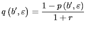
Hence, using Theorem 1, we obtain that:
Footnotes
* We thank Cristina Arellano, Andy Atkeson, Fernando Broner, Jonathan Eaton, Jonathan Heathcote, Pat Kehoe, Narayana Kocherlakota, Guido Lorenzoni, Andy Neumeyer, Victor Rios-Rull, Mark Wright, and Tom Sargent for helpful comments and suggestions. We also acknowledge comments by participants at seminars and conferences at NYU, CUNY, Federal Reserve Bank of Kansas City, SUNY-Albany, Federal Reserve Bank of Minneapolis, SED 2007 Annual Meeting in Prague, LACEA 2007 Annual Meeting in Bogota, and the CREI-CEPR 2007 Conference on Sovereign Risk in Barcelona. Return to text
1. Neumeyer and Perri used data for Argentina, Brazil, Korea, Mexico and the Philippines. Uribe and Yue added Ecuador, Peru and South Africa, but excluded Korea. Return to text
2. See Neumeyer and Perri (2005), Uribe and Yue (2006) and Oviedo (2005). Return to text
3. See, for example, Aguiar and Gopinath (2006), Arellano (2007), Yue (2006), and Bai and Zhang (2005). Return to text
4. Arellano (2007) obtains a mean debt ratio of 6 percent of GDP assuming an output cost of default such that income is the maximum of actual output or 0.97 of average output while the economy is in financial autarky. Aguiar and Gopinath (2006) obtain a mean debt ratio of 27 percent assuming a cost of 2 percent of output per quarter, but the default frequency is only 0.02 percent (in their model without trend shocks and debt bailouts). Yue (2006) assumes the same output cost in a model with renegotiation calibrated to observed default frequencies, but obtains a mean debt ratio of 9.7 percent of output. Return to text
5. This efficiency loss can be modeled in different ways. We can obtain similar results as the ones shown in this paper by modeling the efficiency loss as resulting from costly sectoral reallocation of capital, given an exogenous amount of aggregate capital, or from foreign inputs that are "superior" to domestic inputs in the sense that they support higher TFP. The efficiency loss can also result from changes in capacity utilization, which can be linked to the choice of imported v. domestic inputs using Finn's (1995) setup. Return to text
6. This price can also be modeled as a terms-of-trade shock with a given stochastic process. Return to text
7. In the model, ![]() is
elastic. Our numerical simulations show that when domestic inputs
are used,
is
elastic. Our numerical simulations show that when domestic inputs
are used, ![]() falls compared to the case when
imported inputs are used. Thus, the effect illustrated in Figure 1
actually underestimates the difference in the productivity of
intermediate goods under the two scenarios at work in our numerical
analysis. Return to text
falls compared to the case when
imported inputs are used. Thus, the effect illustrated in Figure 1
actually underestimates the difference in the productivity of
intermediate goods under the two scenarios at work in our numerical
analysis. Return to text
8. ![]() exists when
the interest rates on a country's saving are sufficiently small
compared to the discount factor, which is satisfied in our paper
since
exists when
the interest rates on a country's saving are sufficiently small
compared to the discount factor, which is satisfied in our paper
since
![]() . Return to text
. Return to text
9. We asbtract from debt renegotiation. See Yue (2006) for a quantitative analysis of sovereign default with renegotiation in which the length of financial exclusion is endogenous, and depends on the amount of reduced debt. Return to text
10. See Cuadra and Sapriza (2007) for an analysis of optimal fiscal policy as a Ramsey problem in the presence of sovereign default in an endowment economy. Return to text
11. Alternatively, we could assume that the default punishment includes exclusion from world capital markets and from the world market of intermediate goods. Return to text
12. Arellano and Kocherlakota (2007) document a positive correlation between private domestic lending rates and sovereign spreads using the domestic lending-deposit spread data from the Global Financial Data. Return to text
13. The values of ![]() used by Aguiar and Gopinath (2006), Arellano (2007), and Yue (2006)
range from
used by Aguiar and Gopinath (2006), Arellano (2007), and Yue (2006)
range from ![]() to
to ![]() . Return to text
. Return to text
14. As mentioned earlier, Aguiar and Gopinath (2006) obtained a higher mean debt ratio ( 27 percent of GDP) assuming a cost of 2 percent of output, but with a default frequency of only 0.02 percent. Return to text
15. Using Mexican data, Mendoza (2007) reports a correlation between GDP and imported inputs of 0.91. Return to text
16. Neumeyer and Perri (2005) and Uribe
and Yue (2006) use average interest rates around 7 percent and set
![]() , and they find that the working
capital constraint is important for business cycle dynamics. Oviedo
(2005) also showed that obtaining significant effects of working
capital in the small open economy RBC model requires high values of
, and they find that the working
capital constraint is important for business cycle dynamics. Oviedo
(2005) also showed that obtaining significant effects of working
capital in the small open economy RBC model requires high values of
![]() and
and ![]() Return to text
Return to text
This version is optimized for use by screen readers. Descriptions for all mathematical expressions are provided in LaTex format. A printable pdf version is available. Return to text