Skip to: [Printable Version (PDF)]

Board of Governors of the Federal Reserve System
International Finance Discussion Papers
Number 968, March 2009 --- Screen Reader Version*

Markup Variation and Endogenous Fluctuations
in the Price of Investment Goods¹

Max Floetotto², Nir Jaimovich³, and Seth Pruitt⁴

NOTE: International Finance Discussion Papers are preliminary materials circulated to stimulate discussion and critical comment. References in publications to International Finance Discussion Papers (other than an acknowledgment that the writer has had access to unpublished material) should be cleared with the author or authors. Recent IFDPs are available on the Web at http://www.federalreserve.gov/pubs/ifdp/. This paper can be downloaded without charge from the Social Science Research Network electronic library at http://www.ssrn.com/.

Abstract:

The two sector model presented in this note suggests a simple structural decomposition of movements in the price of investment goods into exogenous and endogenous sources. The endogenous fluctuations arise in the presence of countercyclical markups which vary differently across the consumption and investment sectors. In turn, the movements in the markups are due to endogenous procyclical net business formation. The model, while being consistent with the countercyclicality of the price of investment goods, suggests that about a quarter of the movement in the price series can be attributed to this endogenous mechanism.

Keywords: Price of investment, business cycle, firm dynamics, markup

JEL classification: E32, L11, L16

1.  Introduction

It is well known that the price of investment goods has been trending down over the last century in the US (see for example Greenwood, Hercowitz, and Krusell (2000) and Cummins and Violante (2002)). It has been argued that this decline accounts for a significant fraction of economic growth during that period. For instance, Greenwood and Krusell (2007) conclude that more than half of postwar growth can be attributed to investment-specific technological progress.

Recent work focuses on the cyclical properties of this price series and has emphasized that in the US (i) the price of investment goods is countercyclical, and that (ii) fluctuations in investment-specific technological progress (the inverse of the price of investment goods in many models) contribute significantly to postwar US business cycles. For example, Greenwood, Hercowitz, and Krusell (2000) suggests that this form of technological change is the source of about 30% of output fluctuations. Similarly, Fisher (2006) and Justiniano and Primiceri (2006) argue that investment-specific technological progress is the most important determinant of output variability.

Motivated by this evidence, we investigate cyclical fluctuations in the price of investment goods that can be attributed to endogenous movements. Specifically, this note studies the role of sector specific countercyclical markups in giving rise to endogenous movements in the price of investment goods. Previous work has alluded to the potential role of markup variations in generating movements in the price of investment goods. For example, Ramey (1996) suggests that a decline in markups might have partially caused the relative price of investment to fall over the postwar period. Similarly, Fisher (2006) points out that while "investment-specific technology shocks could play a key role in short-run fluctuations, the short-run correlations might be driven at least partly by factors other than technological change, such as time-varying markups."

The approach taken here is related to a literature following Hall (1986) which suggests that measured Total Factor Productivity (TFP) has important endogenous components.⁵ As this literature has emphasized, the presence of endogenous components can lead a researcher to overestimate the variance of TFP shocks.⁶ In the same spirit, we propose a mechanism that gives rise to endogenous movements in the price of investment goods, and then quantify its contribution to the cyclicality of investment good prices.

Specifically, Section 2 presents a two-sector dynamic general equilibrium model that builds upon the framework of Jaimovich and Floetotto (2008).⁷ There, a positive shock to the level of technology leads to changes in the number of competitors, which in turn give rise to countercyclical variations in markups. By extending this framework to a two-sector setup we can derive a simple analytical characterization of the price of investment goods. We show that this price is positively related to the ratio between the markup in the investment and consumption sector. The households' desire to smooth consumption implies, as it is common in this class of models, that investment is much more volatile than consumption. Hence, the process of firm entry and exit is more volatile in the investment good sector which in turn implies a relatively bigger movement in the markup of the investment than in the consumption sector. Countercyclical movements in the price of investment goods are thus endogenously generated by the model.

Our model suggests that a quarter of the movement in the price of investment goods can be attributed to the endogenous fluctuations as shown in Section 3. Section 4 illustrates that the model can quantitatively account for the countercyclicality of the price of investment goods. In the context of our model, endogenous fluctuations in sectoral markups are necessary to match this feature of the data.

2.  Technology and Market Structure

This note proposes a simple model that represents a minimal perturbation of the prototype perfect competition two sector real business cycle (RBC) model. This greatly simplifies comparison with existing work and allows for a simple structural decomposition of the price of investment goods. The model is a two-sector version of the model in Jaimovich and Floetotto (2008). There are two sectors of production: consumption and investment. Within each period, capital and labor can be costlessly reallocated from one sector to the other. The setup of the consumption sector will be presented in some detail and the investment sector is exactly analogous.

The Consumption Sector. The sectoral good is produced with a constant-returns-to-scale production function, which aggregates a measure one continuum of industrial goods

$$C_{t}=\left[ \int_{0}^{1}Q_{t}^{c}(j)^{\omega}dj\right] ^{\frac{1}{\omega} },\ \omega\in(0,1)$$

where $Q_{t}^{c}(j)$ denotes output of industry $j$. The elasticity of substitution between any two industrial goods is constant and equals $\frac {1}{1-\omega}$. The consumption good producers behave competitively. In each of the consumption industries, there are $N_{t}^{c}$ firms producing differentiated intermediate goods. A $CES$ function aggregates those to yield the output of industry $j$

$$Q_{t}^{c}(j)=\left( N_{t}^{c}\right) ^{1-\frac{1}{\tau}}\left[ \sum _{i=1}^{N_{t}^{c}}x_{t}^{c}(j,i)^{\tau}\right] ^{\frac{1}{\tau}},\ \tau \in(0,1)$$ (1)

where $x_{t}(j,i)$ is the output of firm $i$ in industry $j$.⁸ The elasticity of substitution between any two goods within an industry is constant and equals $\frac{1}{1-\tau}$. The market structure of each industry exhibits monopolistic competition; each differentiated $x_{t}^{c}(j,i)$ is produced by one firm that sets the price for its good to maximize profits. Finally, it is assumed that the elasticity of substitution between any two goods within an industry is higher than the elasticity of substitution across industries, $\frac{1}{1-\omega}<\frac{1}{1-\tau}$. Each intermediate good, $x_{t} ^{c}(j,i)$, is produced using capital, $k_{t}^{c}(j,i),$ and labor, $h_{t} ^{c}(j,i)$ given a level of technology $z_{t}^{c},$

$$x_{t}^{c}(j,i)=z_{t}^{c}k_{t}^{c}(j,i)^{\alpha}h_{t}^{c}(j,i)^{1-\alpha} -\phi^{c},\ \alpha\in\lbrack0,1]$$ (2)

where the parameter $\phi^{c}>0$ represents an overhead cost. In each period, an amount $\phi^{c}$ of the intermediate good is immediately used up, independent of how much output is produced. As in Rotemberg and Woodford (1996) the role of this parameter is to allow the model to reproduce the apparent absence of pure profits despite the presence of market power. Entry into the existing industries is costless for intermediate producers, and hence a zero-profit condition is satisfied in each period and every industry.

We assume that the log technology shocks follow a stationary first order auto-regressive process

$$\ln z_{t}^{c}=\zeta^{c}\ln z_{t-1}^{c}+\varepsilon_{t}^{c}$$ (3)

It is assumed that $\left\vert \zeta^{c}\right\vert <1,$ and that $\varepsilon_{t}^{c}$ is a normally distributed random variable, with a mean of zero and standard deviation $\sigma_{\varepsilon}^{c}$.

The sectoral good producer solves a static optimization problem that results in the usual conditional demand for each industrial good, $Q_{t}^{c}(j)$, where $p_{t}^{c}(j)$ is the price index of industry $j$ at period $t$ and $P_{t}^{c}$ is the price of the consumption good at period $t$,

$$Q_{t}^{c}(j) =\left[ \frac{p_{t}^{c}(j)}{P_{t}^{c}}\right] ^{\frac {1}{\omega-1}}C_{t}$$ (4)

$$P_{t}^{c} =\left[ \int_{0}^{1}p_{t}^{c}(j)^{\frac{\omega}{\omega-1} }dj\right] ^{\frac{\omega-1}{\omega}}.$$ (5)

Denoting the price of good $i$ in industry $j$ in period $t$ by $p_{t} ^{c}(j,i)$, the conditional demand faced by the producer of each $x_{t} ^{c}(j,i)$ variant is similarly defined as

$$x_{t}^{c}(j,i) =\left[ \frac{p_{t}^{c}(j,i)}{p_{t}^{c}(j)}\right] ^{\frac{1}{\tau-1}}\frac{Q_{t}^{c}(j)}{N_{t}^{c}}$$ (6)

$$p_{t}^{c}(j) =\left( N_{t}^{c}\right) ^{1-\frac{1}{\tau}}\left[ \sum_{i=1}^{N_{t}^{c}}p_{t}^{c}(j,i)^{\frac{\tau}{\tau-1}}\right] ^{\frac{\tau-1}{\tau}}.$$

Using (4) and (6), the conditional demand for good $x_{t}^{c}(j,i)$ at period $t$ can then be expressed in terms of the consumption good as

$$x_{t}^{c}(j,i)=\left[ \frac{p_{t}^{c}(j,i)}{p_{t}^{c}(j)}\right] ^{\frac {1}{\tau-1}}\left[ \frac{p_{t}^{c}(j)}{P_{t}^{c}}\right] ^{\frac{1} {\omega-1}}\frac{C_{t}}{N_{t}^{c}}.$$

The Elasticity of Demand. In the model above, there is a continuum of industries within each sector, but within each industry the number of operating firms is finite. While an individual firm's decisions have no effect on the general price level $P_{t}^{c}$, they do affect the industrial price level $p_{t}^{c}(j).$ The resulting price elasticity of demand is then a function of the number of firms within a industry, $N_{t}^{c}$. In a symmetric equilibrium, the elasticity becomes

$$\eta_{x^{c}(j,i)p^{c}(j,i)}(N_{t}^{c})=\frac{1}{\tau-1}+\left[ \frac {1}{\omega-1}-\frac{1}{\tau-1}\right] \frac{1}{N_{t}^{c}}$$ (7)

implying that an increase in $N_{t}^{c}$ leads to a more elastic demand curve. At the solution to the monopolistic firm's problem, marginal revenue equals marginal cost

$$\frac{p_{t}^{c}(j,i)}{MC_{t}^{c}(j,i)}=\mu^{c}(N_{t}^{c})=\frac{(1-\omega )N_{t}^{c}-(\tau-\omega)}{\tau(1-\omega)N_{t}^{c}-(\tau-\omega)} >1.$$ (8)

Note that the markup function is monotonically decreasing in the number of firms, i.e. $\frac{d\mu^{c}}{dN^{c}}<0$. We assume that the economy's technology is symmetric with respect to all intermediate inputs and hence we focus on symmetric equilibria, $\forall(j,i)\in\lbrack0,1]$x$[1,N_{t}]:$ $x_{t}^{c}(j,i)=x_{t}^{c}$, $k_{t}^{c}(j,i)=k_{t}^{c}$, $h_{t}^{c} (j,i)=h_{t}^{c}$, $p_{t}^{c}(j,i)=p_{t}^{c}$, $N_{t}^{c}(j)=N_{t}^{c}$. Total capital and hours in the consumption sector are then given by $K_{t}^{c} =N_{t}^{c}k_{t}^{c}$ and $H_{t}^{c}=N_{t}^{c}h_{t}^{c}$ respectively. Finally, in the symmetric equilibrium, a zero-profit condition is imposed in every sector in every period implying that variable profits cover the fixed cost in each period

$$\left( \mu_{t}^{c}-1\right) x_{t}^{c}=\phi^{c}.$$ (9)

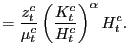
The number of firms per industry and aggregate final consumption can then be found by using (2) and the zero-profit condition (9).⁹

$$N_{t}^{c} =z_{t}^{c}\left( \frac{K_{t}^{c}}{H_{t}^{c}}\right) ^{\alpha }H_{t}^{c}\left[ \frac{\mu_{t}^{c}-1}{\mu_{t}^{c}\phi^{c}}\right]$$ (10)

$$C_{t} =\frac{z_{t}^{c}}{\mu_{t}^{c}}\left( \frac{K_{t}^{c}}{H_{t}^{c} }\right) ^{\alpha}H_{t}^{c}.$$ (11)

We use $P_{t}^{c}$ as the numeraire and set it to $1$. This implies that the price charged by an intermediate producer in the consumption sector is also $1$ in a symmetric equilibrium.

The Investment Sector. The setup in the investment good sector is analogous to the consumption sector. There is a continuum of industries, each with a finite number $N_{t}^{i}$ of intermediate producers. The investment good, the industrial goods, and the differentiated goods are thus produced according to

$$I_{t} =\left[ \int_{0}^{1}Q_{t}^{i}(j)^{\omega}dj\right] ^{\frac {1}{\omega}},\ \omega\in(0,1)$$

$$Q_{t}^{i}(j) =\left( N_{t}^{i}\right) ^{1-\frac{1}{\tau}}\left[ \sum_{i=1}^{N_{t}^{i}}x_{t}^{i}(j,i)^{\tau}\right] ^{\frac{1}{\tau}} ,\ \tau\in(0,1)$$

$$x_{t}^{i}(j,i) =z_{t}k_{t}^{i}(j,i)^{\alpha}h_{t}^{i}(j,i)^{1-\alpha} -\phi^{i},\ \alpha\in\lbrack0,1].$$

The solution to the optimization problem leads to an analogous expression for the markup charged in the investment sector $\mu^{i}(N_{t}^{i})=\frac {(1-\omega)N_{t}^{i}-(\tau-\omega)}{\tau(1-\omega)N_{t}^{i}-(\tau-\omega)}>1$ . Total capital and hours in the investment sector are given by $K_{t}^{i} =N_{t}^{i}k_{t}^{i}$ and $H_{t}^{i}=N_{t}^{i}h_{t}^{i}$ respectively. The zero-profit condition holds in every sector in every period, $\left( \mu _{t}^{i}-1\right) x_{t}^{i}=\phi^{i}$, which as above allows us to derive the number of firms per sector and aggregate investment

$$N_{t}^{i} =z_{t}^{i}\left( \frac{K_{t}^{i}}{H_{t}^{i}}\right) ^{\alpha }H_{t}^{i}\left[ \frac{\mu_{t}^{i}-1}{\mu_{t}^{i}\phi^{i}}\right]$$

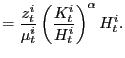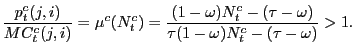
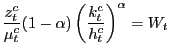
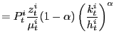
$$I_{t} =\frac{z_{t}^{i}}{\mu_{t}^{i}}\left( \frac{K_{t}^{i}}{H_{t}^{i} }\right) ^{\alpha}H_{t}^{i}.$$ (12)

The Price of Investment. In this economy capital and labor are mobile across sectors and industries. In equilibrium, factor prices have to be equalized in the consumption and investment sector.

$$\frac{z_{t}^{c}}{\mu_{t}^{c}}(1-\alpha)\left( \frac{k_{t}^{c}}{h_{t}^{c} }\right) ^{\alpha}=W_{t} =P_{t}^{i}\frac{z_{t}^{i}}{\mu_{t}^{i}} (1-\alpha)\left( \frac{k_{t}^{i}}{h_{t}^{i}}\right) ^{\alpha}$$ (13)

$$\frac{z_{t}^{c}}{\mu_{t}^{c}}\alpha\left( \frac{k_{t}^{c}}{h_{t}^{c}}\right) ^{\alpha-1}=R_{t} =P_{t}^{i}\frac{z_{t}^{i}}{\mu_{t}^{i}}\alpha\left( \frac{k_{t}^{i}}{h_{t}^{i}}\right) ^{\alpha-1}$$ (14)

This allows us to derive a simple expression for the price of investment by solving (13) or (14) for the price of investment goods $P_{t}^{i}=\left( \frac{z_{t}^{c}}{z_{t}^{i}}\right) \left( \frac{\mu_{t}^{i}}{\mu_{t}^{c}}\right) \left( \frac{k_{t}^{c}} {h_{t}^{c}}\right) ^{\alpha}\left( \frac{k_{t}^{i}}{h_{t}^{i}}\right) ^{-\alpha}$ . This, however, can be simplified further by combining (13) and (14) which yields the well known result that the capital labor ratio is the same in both industries, $\frac{k_{t}^{c}}{h_{t}^{c}}=\frac{k_{t}^{i}}{h_{t}^{i}}$. The price of investment then becomes

$$P_{t}^{i}=\left( \frac{z_{t}^{c}}{z_{t}^{i}}\right) \left( \frac{\mu _{t}^{i}}{\mu_{t}^{c}}\right) .$$ (15)

The first term is standard: when productivity in the investment sector increases relative to the consumption sector, investment goods become cheaper in terms of consumption goods. The second term, however, is a result of the particular sectoral structure that we have assumed. When the investment sector becomes more competitive relative to the consumption sector, i.e. $\frac {\mu_{t}^{i}}{\mu_{t}^{c}}$ falls, the price of investment falls. This equation is the basis of our quantitative exercise in the next section.

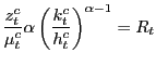
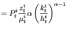
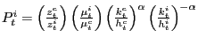
3.  Decomposing the Price of Investment

Using a circumflex to denote log deviations from the steady state, (15) can be expressed as

$$\hat{p}_{t}=\hat{\mu}_{t}^{_{i}}-\hat{\mu}_{t}^{c}+\hat{z}_{t}^{c}-\hat{z} _{t}^{i}.$$ (16)

While the price of investment is observable, all terms on the right hand side of the equation are latent. However, the model's equilibrium conditions imply that we can express $\hat{\mu}_{t}^{_{i}}$ and $\hat{\mu}_{t}^{c}$ as functions of observable data. Taking the consumption sector as an example, one can derive that $\hat{\mu}_{t}^{c} = \left( \frac{1-\tau^{c}\mu^{c}}{\tau ^{c}\mu^{c}}\right) \hat{c}_{t}$ or $\hat{\mu}_{t}^{c} = A\hat{c}_{t}$.¹⁰ Together with the equivalent expression for the investment sector, $B\hat{\imath}_{t}$, we can restate (16) as

$$\hat{p}_{t}=B\hat{\imath}_{t}-A\hat{c}_{t}+\hat{z}_{t}^{c}-\hat{z}_{t} ^{i}.$$ (17)

Our structural decomposition builds on equation (17) as we can express the variance in the price of investment goods as

$$(\hat{p}_{t})= (B\hat{\imath}_{t}-A\hat{c}_{t} )+ (\hat{z}_{t}^{c}-\hat{z}_{t}^{i})+2\times (B\hat{\imath }_{t}-A\hat{c}_{t},\hat{z}_{t}^{c}-\hat{z}_{t}^{i}).$$ (18)

Calibrating the scalars A and B. Note that four parameters - $\mu^{c}$ $\mu^{i}$, $\tau^{c}$ and $\tau^{i}$ - are required to assign values to $A$ and $B$. First, there is, to the best of our knowledge, no clear evidence on the average size of markups in each of the sectors. Similar to Jaimovich and Floetotto (2008), we calibrate the steady state value of the value added markup to $1.3$ in both sectors. Second, we have to choose values for $\tau^{c}$ and $\tau^{i}$, the parameters that determine the elasticity of substitution between differentiated goods in the consumption and investment sector. We calibrate these parameters as follows. Taking the consumption sector as an example, use (8) to find $N_{t} ^{c}=\left( \frac{\tau^{c}-\omega^{c}}{1-\omega^{c}}\right) \frac{\mu _{t}^{c}-1}{\tau^{c}\mu_{t}^{c}-1}$ . Log linearization then leads to an expression for the elasticity of the number of firms with respect to that sector's output,

$$\hat{n}_{t}^{c}=\left( \frac{1-\tau^{c}}{\tau^{c}(\mu^{c}-1)}\right) \hat {c}_{t}.$$ (19)

Using this expression, data on $\hat{n}_{t}^{c}$ and $\hat{c}_{t}$ as well as our calibration of $\mu^{c}$, we can estimate $\tau^{c}$ from the elasticity of the number of firms in the consumption sector with respect to the sector's output.¹¹

This estimation requires time series of the number of operating firms in the consumption and investment sector. As our measure of the number of competitors we use the number of establishments in thirteen non-agricultural major industry groups (referred to as "supersectors") running over 1992:3 - 2007:2 from the BLS Business Employment Dynamics database.¹² We weight each industry group by its average share of annual payrolls as calculated in data from the Small Business Administration (SBA).¹³ We then divide the major industry groups into consumption and investment sectors by modifying the procedure of Harrison (2003): using BEA Input-Output Use tables, we determine the share of each major industry group's product going towards consumption or investment.¹⁴ This procedure provides us with a quarterly time series of establishments in the consumption and the investment sector, $N_{t}^{c}$ and $N_{t}^{i}$; for more details on the data construction, please refer to the data appendix A.¹⁵

We now estimate the elasticities in (19) and the analogous expression for the investment sector by regressing $\hat{n}_{t}^{c}$ on $\hat{c}_{t}$ and $\hat{n}_{t}^{i}$ on $\hat{i}_{t}$, respectively, as shown in Table 1.¹⁶

Note there is only slight difference between the OLS and IV estimates and so we use the former. These estimates imply that $\tau^{c} = 0.867$ and $\tau^{i}=0.923$. Maintaining our assumption that $\mu^{c}=\mu ^{i}=1.3$, we find that $A=-0.0487$ and $B=-0.072$.

Decomposition. The price of investment goods can be decomposed easily using (18) and the values found for $A$ and $B$. We find that about 28% of the variation in the price of investment are due to the endogenous time-variation in markups. Here, we use a time series on the price of investment coming from Fisher (2006).¹⁷ It is important to note that none of the results above require imposing any restrictions on the model's specification of household behavior. The simple expression for the price of investment goods can de derived from the assumptions on technology alone.

4.  Calibration and Simulation

In order to simulate the economy we need to close the model by specifying the household side. It is well known that the sectoral comovement of hours worked does not arise in the benchmark two sector model with separable preferences as in King, Plosser, and Rebelo (1988).¹⁸ We use the results in Jaimovich and Rebelo (forthcoming) who show that this failure can be remedied by assuming a utility function with a weak short-run wealth effect on the labor supply such as the one proposed in Greenwood, Hercowitz, and Huffman (1988).

At each point in time the economy is inhabited by a continuum of identical households. The mass of households is normalized to one. It is assumed that the representative agent has preferences over random streams of consumption and leisure. The representative agent chooses a sequence of consumption, hours and investments in capital to solve

$$\max_{\left\{ H_{t},C_{t},K_{t+1}\right\} }E_{0}\sum_{t=0}^{\infty}\beta ^{t}\log\left( C_{t}-\frac{\theta}{1+\frac{1}{\chi}}H_{t}^{1+\frac{1}{\chi} }\right)$$

subject to the sequential budget constraint and the law of motion for capital

$$C_{t}+P_{t}^{i}I_{t} =R_{t}K_{t}+W_{t}H_{t}+\Pi_{t}$$

$$K_{t+1} =(1-\delta)K_{t}+I_{t}$$

where the initial capital stock is given and equal to $K_{0}$. $C_{t}$ and $H_{t}$ denote consumption and hours worked by the household in period $t$. $\beta\in(0,1)$ and $\delta\in(0,1)$ denote the subjective time discount factor and the depreciation rate of capital, $\chi\geq0$ is the labor supply elasticity and $\theta>0$. Households own the capital stock and take the equilibrium rental rate, $R_{t}$, and the equilibrium wage, $W_{t}$, as given. Finally, households own the firms and receive their profits, $\Pi_{t}$.

We adopt a standard calibration of the parameters in the model - see Table 2.

In order to simulate the model we also need to specify the parameters governing the stochastic process of $z_{t}^{c}$ and $z_{t}^{i}$. We use the model's equilibrium conditions to identify the technology shocks in the two sectors. Log-linearizing equations (11) and (12) and employing the exact same substitutions used to derive (17) leads to

$$\hat{z}_{t}^{c} =(1+A)\hat{c}_{t}-\alpha\left( \hat{k}-\hat{h}\right) -\hat{h}_{t}^{c}$$ (20)

$$\hat{z}_{t}^{i} =(1+B)\hat{\imath}_{t}-\alpha\left( \hat{k}-\hat {h}\right) -\hat{h}_{t}^{i}.$$ (21)

To construct sector specific hours, $H_{t}^{c}$ and $H_{t}^{i}$, we again use the equilibrium conditions of the model as the price of investment goods equals

$$P_{t}^{i}=\frac{C_{t}}{H_{t}^{c}}\frac{H_{t}^{i}}{I_{t}}=\frac{C_{t}}{I_{t} }\frac{\left( H_{t}-H_{t}^{c}\right) }{H_{t}^{c}},$$

which follows from (11) and (12). Hence, using data on $P_{t}^{i},$ $C_{t},$ $I_{t},$ and $H_{t}$ we can construct a series of $H_{t}^{c}$ and $H_{t}^{i}$ that together with (20) and (21) allow us to estimate $\hat{z}_{t}^{c}$ and $\hat{z}_{t}^{i}$. For $\hat {z}_{t}^{c}$ we estimate the AR1 coefficient $\zeta^{c}$ to equal $0.83$ and a standard deviation $\sigma(\varepsilon_{t}^{c})$ of $0.0078$. Similarly, for $\hat{z}_{t}^{i}$ we estimate $\zeta^{i}=0.84$ and $\sigma(\varepsilon_{t} ^{i})=0.0068$. Finally, we find a correlation $\rho(\varepsilon_{t} ^{c},\varepsilon_{t}^{i})$ of $0.605$.¹⁹

Results of Simulation. Panel I in Table 3 reports moments for the US.²⁰ Our benchmark model (Panel II) produces a price of investment series that is countercyclical with a similar magnitude to the one observed in the data. The model underperforms with respect to the volatility of the series: the ratio of standard deviations of the price of investment to output is $1.07$ in the data while this ratio equals $0.75$ in the model. With respect to other variables of interest, the performance of the model is rather standard. Investment is more volatile than output, consumption is less volatile than output, and the model underestimates the volatility of hours worked. Interestingly, the benchmark model (Panel II) generates a correlation between the hours in the two sectors and output that resembles the estimates we obtain in the data.

In order to assess the role of the endogenous markups in generating this negative correlation, Panel III reports the results of the same model with the same technology shocks where the markup is a constant. Hence, the only difference between Panels II and III is along the mechanism emphasized in this note, i.e. the endogeneity of the markup. Note from Panel III that the model generates a price of investment time series that is both (i) less volatile than in the benchmark model and, more importantly, (ii) positively correlated with output. Hence, endogenous movements in the markup are necessary for the model to generate a countercyclical process of the price of investment goods.

5.  Conclusion

This note formulates a simple structural two sector model in a general equilibrium framework in which technology shocks induce the entry and exit of competitors. Endogenous variation in the number of operating firms in the two sectors leads to endogenous variation in the degree of competition over the business cycle. This model economy implies that the price of investment goods can be decomposed into an exogenous component as well as an endogenous component that results from the entry and exit of firms. Based on this decomposition, the note suggests that about a quarter of the variation in the price of investment in the US is due to this interaction. Moreover, the model, when simulated, accounts for the countercyclicality of the price of investment goods. We show that, within our model, endogenous fluctuations in the markups are necessary to match this feature of the data.

The model in this note represents a minimal perturbation of the prototype perfect competition two sector real business cycle model. This greatly simplifies comparison with existing work and allows for a simple structural decomposition of the price of investment goods. However, this simplicity is purchased at the cost of descriptive realism such as the assumption of a symmetric model with no heterogeneity in the size of competitors. Moreover, we do not consider various other elements (such as sector specific capacity utilization and labor hoarding) that could generate endogenous movements in the price of investment goods. We leave these extensions for future research.

Table 1.  Estimation

	OLS: $\hat{n}^c$	OLS: $\hat{n}^i$	IV: $\hat{n}^c$	IV: $\hat{n}^i$
$\hat{c}$	0.513 (0.158)		0.535 (0.178)
$\hat{i}$		0.278 (0.035)		0.320 (0.031)
$R^2$	0.153	0.514	0.155	0.502

Note: OLS and IV estimates; White standard errors in parentheses. Data for dependent variables are described in the text; data for $\hat{c}$ and $\hat{i}$ are log-deviations from HP filter (smoothing parameter 1600) for consumption series PCECC96 and investment series FPIC96, from FRED database at Federal Reserve Bank of St. Louis. IV estimation is 2SLS using a lag of the RHS variable. Constants (not shown) are insignificant. Data run over 1992:3-2007:2.

Table 2.  Calibration

	Parameter	Value
$\mu^{\ast}-1$	Markup in steady state	30%
$\tau^{c}$	Elasticity within industry (consumption sector)	0.87
$\tau^{i}$	Elasticity within industry (investment sector)	0.92
$\alpha$	Capital share	0.30
$H^{\ast}$	Time spent working	0.33
$\beta$	Time discount factor	0.99
$\delta$	Depreciation rate	0.025

Note: The calibration of $\mu$, $\tau^{c}$ and $\tau^{i}$ is explained in the main text. The value of $\omega^{c}$ and $\omega^{i}$ do not matter for the results. The AR(1) parameter on productivity in the two sectors are estimated to be $\zeta^{c}=0.83$ and $\zeta^{c}=0.84$ while the shocks have standard deviations $\sigma\left( \varepsilon_{t}^{c}\right) =0.0078$, $\sigma\left( \varepsilon_{t}^{i}\right) =0.0068$. The correlation between the shocks is $\rho\left( \varepsilon_{t}^{c},\varepsilon_{t}^{i}\right) =0.61$ . The remaining parameters are standard.

Table 3.  Data and Model Moments

	I - Data: $\sigma\left( x\right)$	I - Data: $\sigma\left( x\right) /\sigma\left( y\right)$	I - Data: $\rho\left( x,y\right)$	II - Benchmark: $\sigma\left( x\right)$	II - Benchmark: $\sigma\left( x\right) /\sigma\left( y\right)$	II - Benchmark: $\rho\left( x,y\right)$	III - Constant Markups: $\sigma\left( x\right)$	III - Constant Markups: $\sigma\left( x\right) /\sigma\left( y\right)$	III - Constant Markups: $\rho\left( x,y\right)$
Output (y)	0.015	1	1	0.018	1	1	0.017	1	1
Consumption	0.012	0.80	0.85	0.011	0.59	0.85	0.012	0.72	0.97
Investment	0.047	3.16	0.87	0.065	3.57	0.86	0.035	2.11	0.87
Hours	0.018	1.17	0.78	0.011	0.60	1.00	0.010	0.60	1.00
Hours (C Sector)	0.012	0.80	0.48	0.006	0.33	0.32	0.006	0.35	0.87
Hours (I Sector)	0.037	2.48	0.86	0.049	2.69	0.91	0.030	1.82	0.94
Price of Investment	0.016	1.07	-0.39	0.014	0.75	-0.32	0.008	0.48	0.56
Markups (C Sector)				0.001	0.06	-0.85
Markups (I Sector)				0.012	0.65	-0.86

Note: Second moments of data, benchmark model, and model with constant markups. Benchmark model has endogenous markups. Sectoral hours constructed as described in Section 4. See text for details.

References

Basu, S., and J. G. Fernald (2002): "Aggregate productivity and aggregate technology," European Economic Review, 46(6), 963-991.

Baxter, M. (1996): "Are Consumer Durables Important for Business Cycles?," The Review of Economics and Statistics, 78(1), 147-55.

Christiano, L. J., and T. J. Fitzgerald (1998): "The Business Cycle: It's Still a Puzzle,"Economic Perspectives, 22.

Cummins, J. G., and G. L. Violante (2002): "Investment-Specific Technical Change in the US (1947-2000): Measurement and Macroeconomic Consequences," Review of Economic Dynamics, 5(2), 243-284.

Evans, C. L. (1992): "Productivity shocks and real business cycles," Journal of Monetary Economics, 29(2), 191-208.

Fisher, J. D. M. (2006): "The Dynamic Effects of Neutral and Investment-Specific Technology Shocks," Journal of Political Economy, 114(3), 413-451.

Greenwood, J., Z. Hercowitz, and G. W. Huffman (1988): "Investment, Capacity Utilization, and the Real Business Cycle," American Economic Review, 78(3), 402-17.

Greenwood, J., Z. Hercowitz, and P. Krusell (2000): "The role of investment-specific technological change in the business cycle," European Economic Review, 44(1), 91-115.

Greenwood, J., and P. Krusell (2007): "Growth accounting with investment-specific technological progress: A discussion of two approaches," Journal of Monetary Economics, 54(4), 1300-1310.

Hall, R. E. (1986): "Market Structure and Macroeconomic Fluctuations," Brookings Papers on Economic Activity, 2, 285-338.

Hall, R. E. (1988): "The Relation between Price and Marginal Cost in U.S. Industry," Journal of Political Economy, 96(5), 921-47.

Hall, R. E. (1990): "The Invariance Propereties of Solow's Productivity Residual," in Growth, Productivity, and Unemployment, ed. by P. Diamond. MIT Press.

Harrison, S. G. (2003): "Returns to Scale and Externalities in the Consumption and Investment Sectors," Review of Economic Dynamics, 6(4), 963-976.

Hornstein, A., and J. Praschnik (1997): "Intermediate inputs and sectoral comovement in the business cycle," Journal of Monetary Economics, 40(3), 573-595.

Huffman, G. W., and M. A. Wynne (1999): "The role of intratemporal adjustment costs in a multisector economy," Journal of Monetary Economics, 43(2), 317-350.

Jaimovich, N., and M. Floetotto (2008): "Firm Dynamics, Markup Variations, and the Business Cycle," Journal of Monetary Economics, 55(7), 1238-1252. 14

Jaimovich, N., and S. Rebelo (forthcoming): "Can News About the Future Drive the BusinessCycle?," American Economic Review.

Justiniano, A., and G. E. Primiceri (2006): "The Time Varying Volatility of Macroeconomic Fluctuations," Nber working papers, National Bureau of Economic Research, Inc.

Kim, K. H. (2006): "Is Investment-Specific Technological Change Really Important for Business Cycles?," Discussion paper, UCSD.

King, R. G., C. I. Plosser, and S. T. Rebelo (1988): "Production, growth and business cycles: I. The basic neoclassical model," Journal of Monetary Economics, 21(2-3), 195-232.

King, R. G., and S. T. Rebelo (1999): "Resuscitating real business cycles," in Handbook of Macroeconomics, ed. by J. B. Taylor, and M. Woodford, vol. 1 of Handbook of Macroeconomics, chap. 14, pp. 927-1007. Elsevier.

Long, Jr., J. B., and C. I. Plosser (1983): "Real Business Cycles," The Journal of Political Economy, 91(1), 39-69.

Ramey, V. A. (1996): "Can Technology Improvements Cause Productivity Slowdowns? Comment," in NBER Macroeconomics Annual, vol. 11, pp. 268-274. The University of Chicago Press.

Rotemberg, J. J., and M.Woodford (1996): "Imperfect Competition and the Effects of Energy Price Increases on Economic Activity," Journal of Money, Credit and Banking, 28(4), 550-77.

A  Appendix

Using the BLS data, we arrive at the total number of establishments in a supersector by adding Expansions (businesses that were already in existence and added employees) to Contractions (businesses that were already in existence and shed employees) to Openings (businesses that came into existence) and then subtract Closings (businesses that closed).

In order to weight the number of establishments according to their economic importance we use data on annual payrolls for each major industry group from the Small Business Administration (SBA), for 1988-2005. In its raw form, the SBA has data for twenty large non-agricultural industry groups. These twenty groups are a subpartition of the partition of thirteen above. We hence add these twenty sectors up to get values of the annual payroll for the thirteen BLS supersectors. The average ratio of one major industry group's payroll to the sum of all groups' payrolls is then the group weight, and we use these to calculate normalized establishment counts for the major industry groups. These weights do no vary appreciably between 1988 and 2005.

From the BEA Input-Output Use table, we are able to calculate the amount of output used for Personal Consumption Expenditure or for Fixed Private Investment for eighty-four non-agricultural industries similar to 2-digit SIC industries. Adding up the industries within each major industry group, we arrive at a value of Personal Consumption Expenditure and Fixed Private Investment for the group. We then define the group's consumption sector share as (Personal Consumption Expenditure)/(Personal Consumption Expenditure plus Fixed Private Investment), while the investment sector share is Fixed Private Investment over the same denominator.

Footnotes

1.  First version: May 2008. Return to text

2.  mailto:[email protected]  Return to text

3.  mailto:[email protected] Return to text

4.  mailto:[email protected] Return to text

5.  See, for example, Hall (1988), Hall (1990), as well as Basu and Fernald (2002). Return to text

6.  Similarly, Kim (2006) finds that investment-specific technology shocks are Granger-caused by variables used in Evans (1992)'s analogous finding for Solow residuals. Return to text

7.  Previous work on two-sector neoclassical models includes, among others, Long and Plosser (1983), Baxter (1996), Hornstein and Praschnik (1997), Huffman and Wynne (1999), and Harrison (2003). Return to text

8.  The term $N^{1-\frac{1}{\tau}}$ in (1) implies that there is no variety effect in the model. This allows us to isolate the effect of markup varaitions on the price of investment goods. Return to text

9.  Multiply (2) with $N_{t}^{c}$ and use the zero-profit condition to plug in for $x_{t}^{c}$. In order to find $C_{t}$, multiply (10) by $x_{t}^{c}$ and use the zero-profit condition again. Return to text

10.  Use the equilibrium conditions of the model to show that $C_{t}(\tau^{c}\mu^{c}-1)(1-\omega^{c})=\phi^{c}(\tau^{c}-\omega^{c})$ and log linearize. Return to text

11.  The equivalent expression in the investment sector is $\hat{n}_{t}^{i}=\left( \frac{1-\tau^{i}}{\tau^{i}(\mu^{i}-1)}\right) \hat{\imath}_{t}.$  Return to text

12.  Jaimovich and Floetotto (2008) argue that changes in the number of establishments might be a better measure of changes in the number of competitors in the economy. Return to text

13.  The SBA has data on estimated receipts and employment as well; our results are robust to using either of these instead of payrolls. Return to text

14.  These shares are virtually identical regardless of the Use table year. Return to text

15.  For example, take the Transportation & Warehousing major industry group. We see that 92% of its output goes to consumption and 8% goes to investment, according to the Use table. This major industry group accounts for 3.38% of aggregate payrolls and has 76,000 establishments in 1992:3. Therefore, it accounts for $0.92\times 0.0338\times76000=2363.296$ consumption sector establishments and $0.08\times0.0338\times76000=205.504$ investment sector establishments in that quarter. Return to text

16.  Deviations come from the Hodrick-Prescott (HP) filter (smoothing parameter set at 1600) on logged data. The implied values of $\tau^{\cdot}$ are robust to using growth rates instead of the HP deviations. Consistent with our proposed mechanism, the data show that fluctuations in the number of investment sector firms are about 58% more volatile than the number of consumption sector firms. Return to text

17.  We thank Jonas Fisher for making these data available to us. Return to text

18.  See the discussion in Christiano and Fitzgerald (1998). Return to text

19.  The estimation is done as follows. We treat $\hat{z}_{t}^{c}$ and $\hat{z} _{t}^{i}$ as first differences from which we can build a level series of the two shocks. One approach would then be to follow King and Rebelo (1999). They assume that $\log z_{t}^{c}$ and $\log z_{t}^{i}$ exhibit a linear trend which they use to construct deviations. Using these approach we then estimate $\zeta^{c}=0.96$ and $\sigma(\varepsilon_{t}^{c})=0.008$, $\zeta^{c}=0.99$, and $\sigma(\varepsilon_{t}^{i})=0.008$ and $\rho(\varepsilon_{t} ^{c},\varepsilon_{t}^{i})=0.56$. When calibrated with these parameters, the model generates a countercyclical price of investment too. However, the resulting series of $\log z_{t}^{c}$ and $\log z_{t}^{i}$ exhibit a non linear trend. Hence, our preferred calibration is based on an estimate that uses a more flexible specification of the trend, i.e. an HP trend. Return to text

20.  We use data from 1955:1-2000:4, including the Fisher (2006) price of investment series. Return to text

This version is optimized for use by screen readers. Descriptions for all mathematical expressions are provided in LaTex format. A printable pdf version is available. Return to text

Home | Economic research and data | Publications and education resources
Accessibility | Contact us
Last update: March 31, 2009