
Board of Governors of the Federal Reserve System
International Finance Discussion Papers
Number 972, May 2009 --- Screen Reader
Version*
Border Prices and Retail Prices
NOTE: International Finance Discussion Papers are preliminary materials circulated to stimulate discussion and critical comment. References in publications to International Finance Discussion Papers (other than an acknowledgment that the writer has had access to unpublished material) should be cleared with the author or authors. Recent IFDPs are available on the Web at http://www.federalreserve.gov/pubs/ifdp/. This paper can be downloaded without charge from the Social Science Research Network electronic library at http://www.ssrn.com/.
Abstract:
We analyze retail prices and at-the-dock (import) prices of specific items in the Bureau of Labor Statistics' (BLS) CPI and IPP databases, using both databases simultaneously to identify items that are identical in description at the dock and when sold at retail. This identification allows us to measure the distribution wedge associated with bringing traded goods from the point of entry into the United States to their retail outlet. We find that overall U.S. distribution wedges are 50-70%, around 10 to 20 percentage points higher than that reported in the literature. We discuss the implications of this for measuring the size of the "pure" tradeables sector, exchange rate pass-through, and real exchange rate determination. We find that distribution wedges are very stable over time but there is considerable variation across items. There is some variation across the country of origin for the imported item, for our major trading partners, but not as much as the cross-item variation. We also investigate the determinants of distribution wedges, finding that wedges do not vary systematically with exchange rates, but are related to other features of the micro data.
Keywords: Prices, distribution, exchange rates
JEL classification: F30
1. Introduction
We analyze retail prices and at-the-dock (import) prices of specific items in the Bureau of Labor Statistics' (BLS) CPI and IPP databases. Previous work has exploited these data separately, using either the CPI (Bils-Klenow (2004) and Nakamura-Steinsson (2007)) or the IPP (Gopinath-Rigobon, 2007). We use both databases simultaneously in order to compare prices of items that are identical in description at the dock and when sold at retail. Our primary statistic of interest is the CPI price relative to import price, a statistic that has confusingly been referred to as both the distribution cost or distribution (or profit) margin in the previous literature. Instead, we prefer to call this gap the distribution wedge because it captures everything that encompasses the gap between the retail price and the price at the dock including both profit margins and local distribution costs.2 We think this term is conceptually appealing because while it is clear that at least one these components is necessary to explain real exchange rate dynamics, it is an open question whether the failure of the law of one price for traded goods is primarily driven by variation in profit margins (Engel 1999) or driven by locals costs of distribution (Burstein, Neves and Rebelo (2005)).3 Unfortunately, we are unable to decompose the distribution wedge into its local cost component and its markup component in a nice, nonparametric way. Nonetheless, the total wedge that we measure is 10-20 larger than previous estimates of the distribution wedge and this implies significantly less exchange rate pass-through to retail prices than previous estimates in the literature. After documenting the size of distribution wedges along several cuts of the data, we investigate the determinants of these wedges.
It is well known
that distribution costs are large. In their authoritative survey,
Anderson and van Wincoop (2004) emphasize the importance of
distribution costs as a crucial component of overall trade costs.
They note, " Trade costs, broadly defined, include all costs
incurred in getting a good to a final user other than the marginal
cost of producing the good itself: transportation costs, policy
barriers, information costs, contract enforcement costs, costs
associated with the use of different currencies, legal and
regulatory costs, and local distribution costs (wholesale and
retail)." They further estimate the contribution of distribution
to overall trade costs: "The 170 percent headline number for
overall trade costs [on an ad valorem tax equivalent basis] breaks
down into 55 percent local distribution costs and 74 percent
international trade costs
![]() " Thus, according to
the evidence in Anderson and van Wincoop, distribution costs for
the United States are large and economically important.
" Thus, according to
the evidence in Anderson and van Wincoop, distribution costs for
the United States are large and economically important.
On the macro side, several recent papers have explicitly analyzed the effects of modeling a distribution sector. Burstein, Neves, and Rebelo (2003), Goldberg and Campa (2006), and Choudri, Faruqee, and Hakura (2005) emphasize the importance of a distribution sector in accounting for exchange rate pass-through. Each of these papers shows that incorporating a distribution sector into an otherwise standard model improves the ability of the model to explain observed rates of exchange rate pass-through. In models without a distribution sector, predicted rates of pass-through are counterfactually high.
More generally, several authors argue that the distribution sector can be crucial for understanding and generating models that display realistic real exchange rate dynamics. Burstein, Eichenbaum and Rebelo (2005) present evidence on the importance of properly accounting for the role of distribution services as a component of the prices of goods traditionally classified as "traded". They undertake an Engel (1999)-style decomposition of real exchange rate movements and document that results from this type of accounting exercise are very different when distribution services are included, at least for several large devaluation episodes. Devereux, Engel, and Tille (2003) incorporate a distribution sector in their work on the welfare effects of moving to a single currency in the euro area. In a series of papers, Corsetti, Dedola, and Leduc have worked extensively on modeling the distribution sector [Corsetti and Dedola (2002), Corsetti, Dedola, and Leduc (2008a, 2008b)]. They revisit several classic questions in international macroeconomics, including exchange rate pass-through, the lack of correlation between the real exchange rate and relative (home-foreign) consumption and the international transmission of real and monetary shocks.4
There is also a large literature in international trade and finance that argues that variable markups are essential for explaining real exchange rate dynamics. Recent papers that contribute to the literature are Atkeson and Burstein (2008), Goldberg and Hellerstein (2008) and Nakamura (2008). The latter two papers examine specific industries to understand the sources of incomplete pass-through to retail prices. Consistent with the theoretical work of Atkeson and Burstein, Goldberg and Hellerstein find that 32%5 of the imperfect pass-through is a result of variable markups at the wholesale level. They also find that retail markup variation is much less important and does not seem to vary systematically with exchange rates. This is consistent with a recent paper by Gopinath, Gourinchas and Hsieh (2008) which finds that border price differences are driven by differences in marginal costs not by variable markups. Despite the importance of variable markups in explaining incomplete pass-through, both industry studies cited above find that local distribution costs explain the majority of incomplete pass-through. Our distribution wedge measure captures the level of these markups, not the changes and while we cannot accurately measure either the level or the change in markups, we show in the next section that under plausible assumptions (about the relative magnitudes of the average markup and local costs and about the amount of markup adjustment at the wholesale level in response to an exchange shock), our estimates of the distribution wedge imply significantly less pass-through into retail prices in response to a large devaluation of the dollar than previous studies have found. In short, the overall size of the aggregate distribution wedge is still important.
There are a handful of estimates of the size of the distribution wedge in the literature. Almost all of these estimates are taken from national input-output tables, and hence are performed at a fairly high degree of aggregation. Burstein, Neves, Rebelo (2003) estimate that distribution wedges for tradable consumption goods are quite large, on average around 40 percent of the retail price of these goods for the United States and 60 percent for Argentina. Their primary source of data is national input-output tables. Unlike us, they attribute 100% of the wedge to distribution costs which is why they refer to it as distribution costs rather than the distribution wedge. This result follows naturally from the fact that they assume in their theoretical model that the distribution sector is perfectly competitive so these firms earn zero profits in equilibrium. Their data work implicitly makes the same assumption because their primary source of data is national input-output tables and these tables are derived under the assumption that all production units have constant returns to scale technologies.6
Goldberg and Campa (2006) document the size of the distribution sector for the Unites States and 20 other OECD countries. Their primary data source is also input-output tables so they are assuming that the entire wedge is due to distribution costs. Across countries, distribution wedges on household consumption goods are between 30 and 50 percent of purchasers prices; the estimate for the United States is 43%. For the eight countries for which Goldberg and Campa have time series data, it is found that distribution wedges are sensitive to exchange rate movements. Bradford and Lawrence (2003) also use input-output sources to measure distribution costs in over 100 consumer categories for the United States and eight other industrialized countries. For the United States, Bradford and Lawrence report wedges as a fraction of producer prices of 68% on average, or 40% as a fraction of purchaser prices. There is considerable variation across categories of items and across countries, with Japan and the United States on the high end.
In this paper, we measure the distribution wedge associated with bringing traded goods from the point of entry into the United States to their retail outlet. An important distinguishing feature of our work is that we compute wedges using micro data. As noted above, we compare prices of specific items at the dock and when sold at retail. A "matching procedure", described in detail in the appendix, verifies that the items being compared are identical in description. To our knowledge, no other study of distribution wedges uses as detailed a data set as ours. This allows for a cleaner calculation of the distribution wedge than was possible before and it allows the further advantage to investigate the determinants of the wedge by comparing it with other observed covariates.
After computing estimates of distribution wedges, we make rough attempts to uncover the determinants of these wedges. Of particular interest, given the focus on this question in the existing literature, is whether wedges vary systematically with exchange rates. Potentially, this can help explain the relative importance of the cost versus margin components. We also relate margins to various features of the micro data, such as the frequency of price changes for an item. This is something papers using input-output data are of course unable to do.
We find that overall distribution wedges are around 50-70% for U.S. data between January 1994- July 2007. This number is about 10 to 20 percentage points higher than that reported by other researchers. Distribution wedges are quite stable over time but vary considerably across items. Margins are typically lower for sale price CPI items, as expected, but do not differ significantly across c.i.f. versus f.o.b. import price basis considerations. Surprisingly, intra-company transfer pricing considerations did not have a sizable effect on the size of distribution wedges. There is some variation across the country of origin for the imported item, for our major trading partners, but not as much as the cross-item variation. We do not find that wedges vary systematically with exchange rates although wedges are well explained by other characteristics of the micro data. We take this lack of correlation with the exchange rate as evidence that the majority of our distribution wedge is capturing distribution costs, not profit margins. If distribution wedges were largely composed of variable wholesale markups and if pricing to market is important, then changes in wedges would strong negatively covary with nominal exchange rate changes.
2. Distribution Margin or Distribution Cost
As mentioned in the introduction, we measure the aggregate wedge between the retail price and the price at the dock - a wedge that includes both retail and distributor markups and local distribution and marketing costs. Unfortunately, despite our intensive work with these rich data sets, we are unable to disentangle these two components in a nice, nonparametric way. One way to proceed is to follow the previous literature (Burstein, Neves and Rebelo 2003) and assume that the distribution wedge is equal to the distribution cost. Given that we measure the distribution wedge to be between 10-20% larger than previous estimates, if we performed a similar exercise to the one done by Burstein, Eichabaum and Rebelo (2005), then one would find that our measured wedge implies significantly less pass-through into retail prices than what Burstein, Eichabaum and Rebelo found. This is shown explicitly in the next section of the paper.
We think, however, that the assumption that the distribution wedge is equal to the distribution cost is unappealing because it contradicts a long empirical IO literature arguing that many firms are imperfectly competitive. Furthermore, if there is no markup, there is no role for markup adjustment, contradicting recent empirical work by Goldberg and Hellerstein (2008) and Nakamura (2008), both of whom find that markup adjustment at the wholesale level is important for explaining incomplete pass-through. Another approach is to make a rough approximation of the relative magnitudes of the markup components and the distribution costs components so that we can consider both margins in the exercise we perform in the next section. To fix ideas consider a simple decomposition of the retail price for a single good:
where ![]() ,
, ![]() ,
, ![]() and
and ![]() are the retail price, the
distribution cost, the price at the dock and the markup.
Concretely, one can imagine the case where the foreign manufacturer
owns the wholesaler in the U.S. as is the case in the Beer
industry. (Goldberg and Hellerstein 2008)
are the retail price, the
distribution cost, the price at the dock and the markup.
Concretely, one can imagine the case where the foreign manufacturer
owns the wholesaler in the U.S. as is the case in the Beer
industry. (Goldberg and Hellerstein 2008) ![]() is
the foreign manufacturer's unit marginal cost,
is
the foreign manufacturer's unit marginal cost, ![]() is the markup the wholesaler charges the retail firm to purchase
the item, and
is the markup the wholesaler charges the retail firm to purchase
the item, and ![]() is the total distribution costs
required to bring the product to market
is the total distribution costs
required to bring the product to market![]() 7 The
distribution wedge is defined as
7 The
distribution wedge is defined as
Consistent with the upper estimates from the empirical IO
literature, assume that unit margins are equal to 25%
![]() 8 This
implies that the fraction of the retail price spent on local
distribution and marketing costs is 35%. Consistent with the
empirical literature highlighting the importance of pricing to
market we also assume that the markup varies negatively with the
exchange rate. Specifically, in response to a 1% unexpected
depreciation of the dollar, we assume that wholesale markup falls
by .317%.9 Interestingly no matter which set of
assumptions one makes the implied pass-through into retail prices
is much less than previous studies found.
8 This
implies that the fraction of the retail price spent on local
distribution and marketing costs is 35%. Consistent with the
empirical literature highlighting the importance of pricing to
market we also assume that the markup varies negatively with the
exchange rate. Specifically, in response to a 1% unexpected
depreciation of the dollar, we assume that wholesale markup falls
by .317%.9 Interestingly no matter which set of
assumptions one makes the implied pass-through into retail prices
is much less than previous studies found.
3. Distribution Wedges, Measuring the Tradeables Sector, and Exchange Rate Pass-Through
One concern about the large US external deficits is that they will eventually boost inflation. Typically the purported effects, some of which are quite dire (Obstfeld and Rogoff, 2005), work through the exchange rate. Such concerns are of course tempered when purely traded goods are a small fraction of our economy. Our estimates of the size of distribution wedges have a direct bearing on this issue. To illustrate, let's map distribution wedges into a calculation of the size of the pure traded goods sector, following the extension of Engel's (1999) simple example by Burstein, Eichenbaum and Rebelo (2005).
Think of the CPI
as a geometric average between the retail price of traded goods
![]() and the prices of nontradable goods
and services
and the prices of nontradable goods
and services ![]() :
:
| (1) |
where ![]() is the weight of nontradables in the
CPI not taking into account distribution wedges. The retail price
of traded goods includes both goods that are actually traded, whose
retail price is
is the weight of nontradables in the
CPI not taking into account distribution wedges. The retail price
of traded goods includes both goods that are actually traded, whose
retail price is ![]() , and traded goods that are
consumed locally, whose retail price is denoted
, and traded goods that are
consumed locally, whose retail price is denoted ![]() . Assume that the retail price of tradables can be
written in Cobb-Douglas form as:
. Assume that the retail price of tradables can be
written in Cobb-Douglas form as:
| (2) |
where ![]() is the share of local goods in
tradable goods.
is the share of local goods in
tradable goods.
Assume that
selling at retail one unit of traded or local goods requires
nontradable distribution services and that the price of
distribution services is the same as the price of nontradable
goods. For simplicity, assume the technology to transform traded
and local goods into retail tradable goods is Cobb-Douglas. Denote
the weight of distribution services by ![]() and for
simplicity assume that it is the same for both traded and local
goods. We also assume that the markup the retailer charges is zero.
What matters for incomplete pass-through is variation in the markup
and the empirical evidence suggests that variation in the retail
markup explains less than 1% of incomplete pass-through. (Goldberg
and Hellerstein 2008).
and for
simplicity assume that it is the same for both traded and local
goods. We also assume that the markup the retailer charges is zero.
What matters for incomplete pass-through is variation in the markup
and the empirical evidence suggests that variation in the retail
markup explains less than 1% of incomplete pass-through. (Goldberg
and Hellerstein 2008).
Consistent with
the discussion in the previous section, we assume that the
distributor of the traded good charges a markup ![]() over the dock price. For simplicity, we assume that there is
perfect competition in the distribution sector of the local good.
These assumptions imply that the retail price of traded and local
goods is given by
over the dock price. For simplicity, we assume that there is
perfect competition in the distribution sector of the local good.
These assumptions imply that the retail price of traded and local
goods is given by
| (3) |
and
| (4) |
where
![]() is the price at the dock
of the traded good and
is the price at the dock
of the traded good and
![]() is the price of the
local good exclusive of distribution costs.
is the price of the
local good exclusive of distribution costs.
Assuming that the price of local goods exclusive of distribution costs is the same as the price of nontradable goods:
| (5) |
Equations 1-5 imply that
| (6) |
where
![]() is the
total weight of nontradables in the CPI basket. Assume that PPP
holds for the purely traded component of the CPI:
is the
total weight of nontradables in the CPI basket. Assume that PPP
holds for the purely traded component of the CPI:
| (7) |
where
![]() is the nominal exchange rate,
is the nominal exchange rate,
![]() is the foreign
price of truly traded goods and
is the foreign
price of truly traded goods and ![]() is a constant of
proportionality. Plugging equation 7 into 6 and taking log
differences gives:
is a constant of
proportionality. Plugging equation 7 into 6 and taking log
differences gives:
| (8) |
Consistent with Goldberg and Hellerstein (2008), Nakamura (2008) and Atkeson and Burstein (2008) we assume that the distributor's markup varies with the exchange rate. This allows us to write changes in the markup in terms of changes in the exchange rate.
| (9) |
where
![]() . We choose v equal to 0.317 (see
table 13 of Goldberg and Hellerstein 2008) which implies that for
every 1% depreciation of the dollar, distributor's markups fall by
0.317%. This is because an exchange rate depreciation leads foreign
firms to change the markup or profit margin they earn per unit sold
in the U.S. Using equations 7 and 8 we can now express CPI
inflation in terms of the exchange rate
. We choose v equal to 0.317 (see
table 13 of Goldberg and Hellerstein 2008) which implies that for
every 1% depreciation of the dollar, distributor's markups fall by
0.317%. This is because an exchange rate depreciation leads foreign
firms to change the markup or profit margin they earn per unit sold
in the U.S. Using equations 7 and 8 we can now express CPI
inflation in terms of the exchange rate
| (10) |
It is easy to see that the smaller the weight that pure tradables have in the CPI, the lower the expected change in the CPI will be in response to a devaluation. Also, the more the distributor's markup responds to changes in the nominal exchange rate the lower pass-through will be.
There are two
mechanisms that are often mentioned in discussions of how U.S. CPI
inflation might be "imported" from abroad. The most common begins
with the concern that large U.S. trade deficits will ultimately
cause the dollar to depreciate sharply against other floating
currencies. More recent discussions explain how CPI inflation might
be imported even when the foreign country has a fixed or managed
exchange rate. Note that both mechanisms are captured by equation
8: the former refers to changes in the first term, while the latter
refers to changes in the second term. In the absence of systematic
markup variation (![]() ), given that these
mechanisms enter the inflation equation in a symmetric way, they
imply the same results for depreciations holding foreign costs
constant and for (equivalent-size) foreign cost increases holding
the nominal exchange rate constant. When markups vary
systematically with the exchange rate then one would expect more
pass-through in the latter case.
), given that these
mechanisms enter the inflation equation in a symmetric way, they
imply the same results for depreciations holding foreign costs
constant and for (equivalent-size) foreign cost increases holding
the nominal exchange rate constant. When markups vary
systematically with the exchange rate then one would expect more
pass-through in the latter case.
To understand
the importance of this paper's measuring the size of U.S.
distribution wedges, let's use equation 9 to do some back of the
envelope calculations. We consider two calibrations. For the first
calibration we follow BER and assume that the distribution wedge is
equal to the distribution cost and that there is no markup
variation. Since we find that the average distribution wedge is
equal to 60%, this implies that ![]() and
and
![]() In the second calibration we follow
the empirical IO literature and assume that
In the second calibration we follow
the empirical IO literature and assume that ![]() and
and
![]() BER (2003) estimate the average
distribution cost in the US to be 45%. In 2006, the share of
services (nontradables) in the US CPI-U was 60% (
BER (2003) estimate the average
distribution cost in the US to be 45%. In 2006, the share of
services (nontradables) in the US CPI-U was 60% (
![]() ). They estimate that the share of
traded goods consumed locally could be as large as 22% of traded
goods (
). They estimate that the share of
traded goods consumed locally could be as large as 22% of traded
goods (
![]() ). This suggests that a lower
bound on the amount of pure tradable goods with BER's estimates is
). This suggests that a lower
bound on the amount of pure tradable goods with BER's estimates is
and an upper bound is
Under our first calibration, since the distribution cost is 60% the lower bound on the purely tradable component of the CPI drops to
with an upper bound is
With such a small tradable component to the CPI that would be guided by PPP, there is less reason to be concerned that U.S. inflation would be highly affected by even a large and sharp depreciation.
Using this lower
bound, we can get a back-of-the-envelope guess at what would happen
to U.S. inflation if there was a big depreciation but foreign
prices remained constant. (Remember that this is equivalent in our
framework to considering a large increase in foreign prices holding
the exchange constant when there is no markup adjustment). Assume
that nontradable good prices in the U.S. grow at 2% a year. Assume
also that we have a 25 unexpected depreciation in the nominal trade
weighted exchange rate, that foreign prices do not change over this
period and that pure traded goods obey PPP. Under the first
calibration this implies that the share of nontradables in the CPI
is ![]()
![]() Then the expected inflation rate using equation 9 gives
Then the expected inflation rate using equation 9 gives
Under the second calibration, the share of nontradables in the CPI
is equal to 79.7% and ![]() Expected inflation
under this scenario is given by
Expected inflation
under this scenario is given by
Using the BER calibration with an estimated 45% distribution margin produces an expected inflation rate of 6%. Therefore our (higher) estimate of distribution wedges lowers the expected pass-through to domestic inflation by 19% relative to BER in the first calibration and by 16% relative to BER under the second calibration. This a non-trivial difference for an economy like the United States which has a low and stable inflation rate. However, the main lesson of both BER and our paper is that when distribution costs and markup adjusted are included, the expected change in the CPI in response to even a very large unexpected depreciation is not that alarming. Excluding distribution costs of course implies much higher expected inflation - our simple example produces inflation rates of around 9% under the first calibration- even greater when local goods are excluded. Of course, with larger unexpected depreciation rates the inflationary implications are larger, e.g., with a 45% depreciation, the expected CPI inflation rate is 7.4% when distribution costs are taken into account.
Qualitatively,with even higher distribution wedges than had previously been reported in the literature, the inflationary consequences for the United States of a large depreciation are even less disastrous. Of course these are simple back of the envelope calculations and do not necessarily emerge from a more desirable general equilibrium analysis.
4. Measuring Distribution Wedges
We measure distribution wedges in two ways. First, using the detailed information on product characteristics in the CPI and IPP databases, we match items at the dock to those sold at retail that are identical in description. Our matching procedure is done on a category by category basis depending on available information, as described in detail in the appendix. Under this procedure we are highly confident that we are comparing at-the-dock prices and retail prices of items that are identical in description. Unfortunately, this procedure also necessitates that we discard a lot of data, either because exact matches did not exist or because there was insufficient evidence to determine the quality of a match.
In light of this last consideration, we check robustness using a second measure of distribution wedges. Under this procedure we construct weighted-average price levels for fairly disaggregated item categories in the CPI and import price data bases. The level of aggregation is by entry level item (ELI) in the CPI, or approximately 10-digit SIC code for imports. We use prices of only those CPI items that we could reliably determine to have been imported rather than made in the United States. This alternative procedure allows us to measure the distribution wedge for item categories such as (imported) " beer", " televisions", and " bananas" . Under this procedure we utilize the prices of many more of the items in the sample but use less of the item-specific information that is contained in the database.
Under both
strategies, the distribution wedge for item category i, ![]() , is calculated as
, is calculated as ![]() =
(CPI
=
(CPI![]() - IPP
- IPP![]() ) /
CPI
) /
CPI![]() , where CPI
, where CPI![]() is the retail price of the item (or
its weighted average price level) and IPP
is the retail price of the item (or
its weighted average price level) and IPP![]() is the
import price.10 We use monthly data from January
1994 to July 2007.
is the
import price.10 We use monthly data from January
1994 to July 2007.
The calculation
of ![]() could be affected by several important
" price basis" considerations.11 The first is whether
the CPI item's price is a sale price or a regular price. Second, is
whether the imported item is priced on a c.i.f. or f.o.b. basis.
Finally, we must distinguish between imports that are intra-company
transfers and those that are arm's length transactions that more
accurately reflect market prices. Each of these could have
non-trivial effects on the distribution wedge. In light of this, we
report results in a few different ways reflecting combinations of
these price bases considerations.
could be affected by several important
" price basis" considerations.11 The first is whether
the CPI item's price is a sale price or a regular price. Second, is
whether the imported item is priced on a c.i.f. or f.o.b. basis.
Finally, we must distinguish between imports that are intra-company
transfers and those that are arm's length transactions that more
accurately reflect market prices. Each of these could have
non-trivial effects on the distribution wedge. In light of this, we
report results in a few different ways reflecting combinations of
these price bases considerations.
In Table 1 we report the median distribution wedge for all items under the first of our measurement procedures. Results using the " matching procedure" described in the appendix are contained in part A of the table, while those of the alternative procedure using weighted average price levels are in part B. For the former we report wedges in four ways: when the CPI price is regular and the import price basis is cif, CPI price is regular and import price is fob, and the analogies for cases in which the CPI price is a sale price. In the upper panels intra-company transfer prices are excluded. In the lower panels we report the same calculations using only the intra-company transfer prices.
4.1 Distribution Wedges: All Items
According to the upper panel of Table 1A, when transfer prices are excluded from the sample the median distribution wedge across all regular-priced CPI items is 0.57 (0.68) for imports priced on a cif (fob) basis. For sale-price CPI items the respective distribution wedges are 0.50 (0.60). The analogous numbers for transfer prices are, contrary to our prior expectations, generally quite similar: 0.58 (0.62) and 0.57 (0.49), as seen in the lower panel of Table 1A.
The distribution wedges reported in Table 1 are distinctly higher than the estimates reported for U.S. consumption goods by other researchers. Burstein, Neves, and Rebelo (2003) estimate U.S. distribution wedges12 to be 42% in 1992 and 43% in 1997, using the national input-output tables. The wedge is about the same when the authors use data from the 1992 U.S. Census of Wholesale and Retail Trade. Goldberg and Campa's (2006) cross-country evidence confirms the 43% estimate of the distribution wedges for all U.S. final household consumption in 1997 (also using national input-output data), estimating that most of this is due to distribution wedges in the wholesale-retail sector rather than transportation. Bradford and Lawrence (2003) report an overall distribution wedge for the United States in 1992 of 40% as a percentage of purchaser price.
4.1.1 Alternative Procedure
Table 1B reports distribution wedges computed under the alternative procedure where we construct weighted-average price levels for fairly disaggregated item categories. These wedges are slightly higher than those obtained from the matching procedure: 0.70 or 0.64 depending on how we weight item categories. This indicates a general robustness to using prices of considerably more items than was possible under the matching procedure.
4.1.2 Stability Over Time
The wedges are quite stable over time. Lumping all items together without distinguishing between cif and fob, sale price or not, etc., our matching procedure gives us wedges of 0.62, 0.67, 0.63, 0.57, 0.59, 0.60, 0.58, 0.61, 0.59, 0.57, 0.58, 0.60, 0.60 and 0.61 in the years 1994 through 2007 respectively. As noted above, a relatively stable overall distribution wedge is also found by Burstein, Neves and Rebelo (2003). This stability of wedges against the backdrop of considerable fluctuations in the dollar foreshadows our finding below concerning the lack of a relationship between distribution wedges and exchange rates.
4.2 Results by Item
In our data sample, there is considerable variation across items, with wedges ranging from around 20 percent to 80 percent. These results are presented in Table 2A for the 21 item categories from which we were able to uncover a sufficient number of high-grade matches (see the appendix tables for the number of observations in each category). The lowest wedges are for televisions, video cameras, VCRs, cameras, telephones and microwave ovens. The highest wedges are found for drugs, our two apparel categories (men's and women's pants), watches, film, and our two fresh foods categories (bananas and tomatoes). As expected, wedges are typically lower for sale price items, and in some cases the difference is nearly 20 percentage points. Wedges do not differ systematically between the cif and fob price basis, though on average fob wedges are higher as expected.
Table 2B reports results by item category when we compute distribution wedges using the alternative procedure.13 Consistent with the results under the matching procedure, the largest wedges are observed for watches, olive oil, and bananas, with wedges for television sets (and alcoholic beverages here) being at the low end. Below we relate the cross-section of distribution wedges to features of the micro data underlying our sample.
4.3 Composition Effects and Results by Brand
The results so far could be masking important composition effects, in principle across brand, time, and country of origin. The item categories above, while certainly disaggregated to some extent, still contain product heterogeneity. There are, for example, the wedges associated with small-screen television sets (13-inch diameter) and those associated with large, high-end televisions. These wedges are averaged together in the results above. If there are important composition effects, it may be misleading to compare our estimates to those of the existing literature, or to compare results across various slices of our own data set.
Concerning the comparison with existing estimates of distribution wedges, note that in his conference discussion of our paper (FRB-NY, December 2007), Ariel Burstein presented results indicating that composition effects do not explain the higher wedges we report relative to BER (2003). That is, Burstein showed that the distribution wedges in the NIPA data used by BER are consistently lower than what we report from the BLS data, category by category.
Furthermore, we compute distribution wedges by brand for cases in which we have at least ten observations. Table 3a reports results for Alcoholic Beverages for the case in which transfer prices are excluded. Table 3b repeats the exercise for beer and television sets. (Confidentiality considerations between the BLS and companies preclude us from naming the actual brands.) Composition effects across brands do not appear to be a predominant factor: distribution wedges for individual brands are in most cases close to the aggregate distribution wedge calculated for all brands together. Television sets are a notable exception (table 3b). Consider the seemingly anomalous result that the wedge associated with fob prices is higher for television sets where there is a sale price in the CPI than for regular-priced CPI televisions, 0.35 versus 0.21. Making the same comparison by brand, we see that in each case the wedge for sale-price televisions is, as expected, lower than for regular-priced items.
4.4 Distribution Wedges by Country-of-Origin
We also calculate distribution wedges based on a different cut of the data. Here we lump together all items that were imported from a particular trading partner and calculate distribution wedges based on the matching procedure. Table 4 presents the results for our major trading partners. wedges range from a low of 0.36 for Japan (for imports priced on an fob basis) to 0.75 for Mexico (cif basis). However, most of the wedges fall within the range of 50% to 60% reported in the all-items tables above.
5. Determinants of Distribution Wedges
We attempt to explain the determinants of distribution wedges by relating the estimates described above to various quantifiable features of the micro data underlying our sample. In terms of broad brush, we go about this with two distinct approaches that examine various " within" and " between" determinants. First is to explain the determinants of distribution wedges across item categories themselves or across exporting countries themselves. Under this approach we compute summary numbers (medians) for a particular item category and explain the variation in (median) distribution wedges across item categories. The other approach is to look within an item category and examine the determinants of distribution wedges across items in that category. We repeat this exercise for particular trading partner countries, to examine the determinants of distribution wedges across all items originating from that particular country.
5.1 Accounting for Variation in Distribution Wedges
As a first pass
at understanding the determinants of distribution wedges, we ask
which of the two components of the wedge, the IPP price or the CPI
price, accounts for more of the movements in the wedge itself? Or
alternatively, we ask are there offsetting movements in the IPP and
CPI prices such that distribution wedges are unrelated to either?
In Table 5 we present the results of a simple decomposition of the
variation in distribution wedges. In particular, we report the
![]() values from three different bivariate
regressions involving, respectively, the IPP price and the CPI
price, the CPI price and the distribution wedge, and the IPP price
and distribution wedge. The variables are in log first-differences,
and all regressions contain a constant but no lags.
values from three different bivariate
regressions involving, respectively, the IPP price and the CPI
price, the CPI price and the distribution wedge, and the IPP price
and distribution wedge. The variables are in log first-differences,
and all regressions contain a constant but no lags.
As with the calculations above, we report results for three different slices of the data: by item category, by year, and by country of origin of the import. The bulk of the evidence presented in Table 5 indicates that variation in the wedge is primarily accounted for by movements in the retail price, with very little due to movements in the import price. In addition, There is very little evidence of a systematic relationship between movements in the IPP price and the CPI price. The latter is consistent with the literature on exchange rate pass-through into the United States. More specifically, these conclusions hold by item category according to Table 5a: only for computer accessories and cameras is significantly more of the variation in the distribution wedge accounted for by the IPP price than the CPI price. This pattern is relatively stable over time, according to Table 5b, though there is a noticeable decline in the contribution of the CPI price in the latter part of the sample. During this period there is a rise in the contribution of the IPP price to the wedge but it is not large.14 Finally, when we perform this simple decomposition by country of origin we see that movements in the CPI price account for more of the variation in wedges than do movements in the IPP price for each trading partner. In addition, only in the case of imports coming from Canada is there a non-zero relationship between movements in the IPP and CPI prices.
5.2 Distribution Wedges, Endogenous Exits, Law of One Price Deviations and Sticky Prices
Next we relate distribution wedges to various features of the BLS micro data. Two of these features are measures of law of one price deviations and price stickiness. They are well-known, and we simply follow the existing literature in calculating them from the BLS micro data. The third feature is our own construct, whose explanation we turn to next.
5.2.1 Endogenous Exits
One striking feature of the micro data in the IPP database is that particular items imported from particular countries are relatively short-lived. We construct a variable that summarizes the short-lived nature of such items, and see if this is systematically related to distribution wedges. We label this new variable the " endogenous exits" ratio. An endogenous exit is said to occur any time (1) the importing company has gone out of business; (2) the BLS industry analyst, in consultation with the company, concludes that a product is " out of scope", indicating that there is no longer a meaningful market for the product; or (3) highly significant changes in quality are made to an existing item. We then count, within each of the item categories used in the matching procedure, the number of items in that category experiencing an endogenous exit during the sample period. The variable of interest, the endogenous exits ratio, is the ratio of this count to the total number of items in that category.15
The unconditional relationship between endogenous exits and distribution wedges is displayed in the scatter plot in the upper left panel of Figure 1. Each dot represents a single item category, for example beer. The relationship is negative, with a simple correlation coefficient of -0.37 and no clear outlier observations. Thus, in our data, item categories with small distribution wedges are those with relatively many endogenous exits. We offer interpretations of this finding below.
5.2.2 Law of One Price Deviations
We next examine the relationship between distribution wedges and deviations from the law of one price for the CPI items used in the matching procedure. Conceptually, if the law of one price is closer to holding in the market for a particular item we may expect that market to be more competitive and hence exhibit smaller distribution wedges. To be specific, we calculate absolute deviations from the law of one price across cities for a particular type of, e.g., television set. Recall that we have already determined particular items to be " identical in description" through our matching procedure. These are the only items whose (cross-city) price we are comparing in this exercise. For each category like televisions we calculate one number: the median law of one price deviation across all of the individual city-pair observations. We then relate this to the distribution wedge already calculated for that item category.
The relationship is depicted in the upper right panel of the figure. There is clearly a positive relationship in our data: categories such as televisions, VCRs, microwave ovens have very small deviations from the law of one price at the retail level; these are also the categories with the smallest distribution wedges.
The tri-variate relationship among distribution wedges, endogenous exits, and law of one price deviations at retail provides some economic insights. In item categories where the distribution wedge is small there is a relatively large amount of product churning or turnover, directly observed at the import stage, either because of significant quality changes or other market forces that render products obsolete relatively quickly. These small-wedge (and high exits) item categories are also those in which market forces keep prices relatively in line with the law of one price at the retail level.
5.2.3 Sticky Prices
Finally we ask whether distribution wedges are related to measures of price stickiness. On a priori grounds, we may expect that the sectors with low wedges and in which the law of one price comes close to holding, are also characterized by relatively flexible prices. This appears to be the case. In the bottom row of the figure we depict scatter plots of distribution wedges against the probability that an item in that category experienced a price change. We calculate these probabilities for both the CPI price (lower left panel) and the IPP price (lower right) of that item. We follow Nakamura and Steinsson (2007) in calculating the probabilities (we include both sales prices and regular prices in our CPI calculations). As seen in the figure, the relationship is affected by a small number of outlier observations. Excluding the outliers, the relationship is strongly negative, -0.42 for CPI and -0.31 for IPP, so that lower wedges are associated with more frequent price changes.16 On the CPI side, the one outlier category is tomatoes, for which prices are quite flexible while distribution wedges are high. This presumably reflects a relatively unique combination of (1) supply-side competition, product homogeneity and low demand elasticities inducing frequent price changes and (2) costly transport and storage needs that keep wedges high. On the IPP side, tomatoes are again an outlier, as are bananas and olive oil.
This simple, non-structural examination of the determinants of distribution wedges suggests an interesting relationship among distribution wedges and three "micro features" of the BLS data: endogenous exits, law of one price deviations, and sticky prices. The relationship points to the likely strong role of factors that we would expect to see influencing distribution wedges - competition, product substitutability, transportation and storage costs.
5.3 Do Distribution Wedges Move Systematically With Exchange Rates?
One of the important goals of Goldberg and Campa (2006) was to examine the relationship between distribution wedges and exchange rate changes. As shown in our example of section 2, there is a simple mapping between distribution wedges and the size of the pure tradeables sector. Thus, a finding that wedges move with exchange rates suggests that exchange rate changes would, all else constant, be associated with a change in the size of this sector.
Campa and Goldberg (2006) report that home currency depreciations are associated with statistically significantly lower distribution wedges in a panel regression containing the United States and 9 European countries. They use national data, at a fairly high level of aggregation, over the period 1995-2001. Their estimates indicate that a 1% real depreciation results in a 0.47 percent decline in the distribution wedge. Such an elasticity of the wedge with respect to exchange rate changes is large enough that it could, in principle, be able to account for much of the discrepancy between our estimates of wedges and those in the existing literature.
As noted above, however, there is prima facie evidence against finding a relationship between distribution wedges and exchange rates in our data. Recall that our average annual distribution wedge across all items during the period 1994-2007 fluctuates between 0.57 and 0.67, with all of the estimates after 1996 lying between 0.57 and 0.61. During this period the dollar moved by a considerable amount: against the currencies of our major trading partners, the dollar first appreciated by more than 20 percent and subsequently depreciated by more than 30 percent. Were we to apply the Goldberg-Campa elasticity to the recent U.S. experience, the large drop in the dollar would have been associated with about a 6 percentage point drop in the distribution wedge, all else constant.
More formally, in Table 6 we present the results of a regression of the change in distribution wedges on the contemporaneous change in the exchange rate, two lagged changes in the exchange rate, and two lagged changes in the foreign CPI.17The data are monthly from January 1994-July 2007. We run the regression on two different cuts of the data, first by item (Table 6A) and second by country of origin of the import item (Table 6B). In the former regression the exchange rate is the trade-weighted value of the dollar, while in the latter regression the exchange rate is the bilateral rate of the dollar against the currency of the exporting country.
We report
coefficient estimates on the contemporaneous exchange rate change
as well as the F-statistic from a test of the null hypothesis that
the exchange rate changes are jointly zero. We also report the
regression R![]() values. According to Table 6A there
is only modest evidence that exchanges rates significantly affect
distribution wedges. In two categories, Drugs and Microwave ovens,
the coefficient on the contemporaneous exchange rate change is
negative and statistically significant. In each case the F-test
indicates that the exchange rate changes are jointly non-zero and,
in the case of drugs, the regression R
values. According to Table 6A there
is only modest evidence that exchanges rates significantly affect
distribution wedges. In two categories, Drugs and Microwave ovens,
the coefficient on the contemporaneous exchange rate change is
negative and statistically significant. In each case the F-test
indicates that the exchange rate changes are jointly non-zero and,
in the case of drugs, the regression R![]() is
sizable. However, for most items the regressions indicate that
there is essentially no relationship between exchange rates and
distribution wedges.
is
sizable. However, for most items the regressions indicate that
there is essentially no relationship between exchange rates and
distribution wedges.
Table 6B repeats
the analysis, this time on a country-by-country basis lumping all
items together. Here we find even less evidence that exchange rate
changes are significant. For Canada, the estimated coefficient on
the contemporaneous exchange rate is large at -0.61, but has a
standard error of 0.4. The F-statistic for the Canadian regression
does indicate that exchange rate changes are jointly non-zero but
the regression ![]() is quite small.
is quite small.
The absence of a significant relationship between distribution wedges and exchange rate changes would seem to contradict Goldberg and Campa (2006). However, the data sets used in the two papers are quite different, with the Goldberg-Campa data set being richer in the cross-country dimension. Our data for the United States, a relatively closed economy, is richer across item categories. No matter how we sliced our data set, however, there was no consistently significant relationship between distribution wedges and exchange rates.
5.4 A Multivariate Empirical Model of Distribution Wedges
We conclude the section with an examination of the joint significance of each of the variables discussed so far in explaining distribution wedges. For each item category, we regress the distribution wedge for product i and time t on several variables:
where BRAND is the brand name of product i, SALE is a zero-one dummy indicating whether the price of the CPI item is a regular price or sale, BUSINESS is also zero-one denoting the type of retail outlet where the item was sold (large retailer or discount store versus small convenience-type of store), PBASIS is the price basis for the imported item (cif versus fob), LOPDEV is the law of one price deviation for the CPI item, and EXITS is the endogenous exit count for that item category. We then repeat this analysis for each country of origin, running the regression above over all items imported from that country.
The results are
depicted in Table 7A (by item) and 7B (by country of origin). We
are primarily interested in the contribution to ![]() of each explanatory variable. These are reported in
square brackets in the cells. We report the
of each explanatory variable. These are reported in
square brackets in the cells. We report the ![]() of
the full model in column 1. These range from just below 0.2 for
some categories up to nearly 0.9 for others. Product BRAND
typically has a sizable contribution to overall
of
the full model in column 1. These range from just below 0.2 for
some categories up to nearly 0.9 for others. Product BRAND
typically has a sizable contribution to overall ![]() values, according to column 2. BUSINESS type and SALE
flag dummies have the expected signs (positive and negative,
respectively) and in some cases contribute significantly to the
overall fit, especially the former variable. Within item category,
law of one price deviations are often negatively related to
distribution wedges. This does not necessarily contradict the
cross-item evidence shown in the scatter plot above. It may be the
case, for example, that this within-category relationship reflects
the effect of a factor such as distance between cities in causing
both a larger deviation from the law of one price and, through
transport costs, smaller distribution wedges. Endogenous EXITs are
typically negative (though there are exceptions here too) and often
significant: within item categories, higher product turnover is
associated with smaller wedges just as in the cross-item results in
the scatter plot.
values, according to column 2. BUSINESS type and SALE
flag dummies have the expected signs (positive and negative,
respectively) and in some cases contribute significantly to the
overall fit, especially the former variable. Within item category,
law of one price deviations are often negatively related to
distribution wedges. This does not necessarily contradict the
cross-item evidence shown in the scatter plot above. It may be the
case, for example, that this within-category relationship reflects
the effect of a factor such as distance between cities in causing
both a larger deviation from the law of one price and, through
transport costs, smaller distribution wedges. Endogenous EXITs are
typically negative (though there are exceptions here too) and often
significant: within item categories, higher product turnover is
associated with smaller wedges just as in the cross-item results in
the scatter plot.
Finally, Table
7B presents the within-country evidence. Once again, ![]() values for the overall model are fairly high, up to
0.75 for items imported from Mexico and China. As in Table 7A,
BRAND considerations tend to be very important while BUSINESS type
and SALE flags again have the expected signs. Endogenous EXITs are
typically unimportant according to the contributions to
values for the overall model are fairly high, up to
0.75 for items imported from Mexico and China. As in Table 7A,
BRAND considerations tend to be very important while BUSINESS type
and SALE flags again have the expected signs. Endogenous EXITs are
typically unimportant according to the contributions to ![]() statistics in brackets.
statistics in brackets.
6. Conclusions: Five Facts about Prices... Retail and At-The-Dock18
Using the detailed information on product characteristics in the CPI and IPP databases of the U.S. Bureau of Labor Statistics, we match items imported into the United States to those sold at retail that are identical in description. We compute the size of the resulting distribution wedge of CPI price relative to import price and then investigate the determinants of these wedges. We also map distribution wedges into a calculation of the size of the pure traded goods sector, and discuss the implications of our findings for exchange rate pass-through.
We find the following,
- Distribution wedges for the United States are large.
Our calculation is in the range of 50-70% for U.S. data between January 1994- July 2007. Wedges are slightly higher under the "alternative procedure" than baseline calculations obtained from the detailed "matching procedure". Back of the envelope calculations using a simple modeling framework of BER (2005) imply that the size of the "pure" tradeables sector in the U.S. is thus in the range of 7-16%.
- Wedges are larger than previously reported.
Our headline number is about 10 to 20 percentage points higher than a consensus estimate of 40-45% which was essentially obtained using NIPA data (Burstein-Neves-Rebelo, Goldberg-Campa, Bradford-Lawrence). This maps into a calculation of the "pure" tradeables sector that is 5 to 10 percentage points lower than the 22% number reported by BER. Differences between our results and those of the exisiting literature appear to be driven by differences in the data sets used, rather than by compositional effects. Since our calculations using the BLS data are built up from the microeconomic level, we hope they provide a cleaner calculation of distribution wedges than was possible before.
- Wedges are stable over time but vary considerably across items.
Under the matching procedure, the average annual distribution wedge across all items is 0.62, 0.67, 0.63, 0.57, 0.59, 0.60, 0.58, 0.61, 0.59, 0.57, 0.58, 0.60, 0.60 and 0.61 in the years 1994 through 2007 respectively. The relative stability of wedges coincides with large fluctuations in the dollar over time. Across item categories, several exhibit low wedges: televisions, video cameras, VCRs, cameras, telephones, microwave ovens, while other categories have high wedges: drugs, apparel (men's, women's pants), watches, film, bananas, tomatoes.
- Wedges do not vary dramatically with exchange rates or across
major exporters.
Our average annual distribution wedge across all items lies between 0.57 and 0.61 during a period when dollar first appreciated by more than 20 percent and subsequently depreciated by more than 30 percent. More formal regression results using the individual item data confirms the lack of a relationship between changes in wedges and exchange rates. When we slice the data by the country of export, most of the wedges fall within the range of 50% to 60%.
- Variation in wedges is explained by proxies for sectoral
characteristics
Between categories, distribution wedges vary negatively with endogenous exits and frequency of price changes, and positively with law of one price deviations in the retail market. Thus, in categories where the wedge is small there is a relatively large amount of product churning or turnover, directly observed at the import stage. This turnover is because significant quality changes are made to the product or because other market forces render that product obsolete relatively quickly. These small-wedge item categories are also those in which market forces lead to relatively frequent price changes and keep prices relatively in line with the law of one price at the retail level. Within categories, wedges are explained by brand effects, the type of retail outlet, and on whether the item is sold at sale price.
References
Anderson, J., van Wincoop, E., 2004. "Trade costs". Journal of Economic Literature 42(3), 691-751.
Atkeson, A., Burstein, A., 2008. "Pricing to market, trade costs, and international relative prices". American Economic Review, forthcoming.
Bils, M., Klenow, P., 2004. "Some evidence on the importance of sticky prices". Journal of Political Economy 112(5), 947-985.
Bradford, S., Lawrence, R., 2003. Paying the price: the cost of fragmented international markets. The Peterson Institute for International Economics.
Burstein, A., Eichenbaum, M., Rebelo, S., 2005. "Large devaluations and the real exchange rate". Journal of Political Economy 113(4), 742-784.
Burstein, A., Neves, J., Rebelo, S., 2003. "Distribution costs and real exchange rate dynamics". Journal of Monetary Economics 52(6), 1189-1214.
Choudri, E., Faruqee, H., Hakura, 2005. "Explaining exchange rate pass-through in different prices". Journal of International Economics 65(2), 349-374.
Corsetti, G., Dedola, L., 2005. "A macroeconomic model of price discrimination," Journal of International Economics 67(1), 129-156.
Corsetti, G., Dedola, L.,Leduc, S., 2008a. "International risk sharing and the transmission of productivity shocks," Review of Economic Studies 75, 443-473.
Corsetti, G., Dedola, L., Leduc, S., 2008b. "Models of high exchange rate volatility and low pass-through," Journal of Monetary Economics, forthcoming.
Devereux, M., Engel, C., Tille, C, 2003. "Exchange rate pass-through and the welfare effects of the euro". International Economic Review 44(1), 223-242.
Engel, C., 1999. "Accounting for real exchange rate changes". Journal of Political Economy 107, 507-538.
Goldberg, L., Campa, J., 2006. "Distribution margins, imported inputs, and the sensitivity of the CPI to exchange rates". Review of Economics and Statistics, forthcoming.
Goldberg, P., Hellerstein, R., 2008. "A framework for identifying the sources of local-currency price stability with an empirical application". working paper.
Gopinath, G., Rigobon, R., 2008. "Sticky borders". Quarterly Journal of Economics 123(2), 531-575.
Gopinath, G., Ishtoki, O., Rigobon, R., 2007. "Currency choice and exchange rate pass-through". American Economic Review, forthcoming.
Gopinath, G., Ishtoki, O., 2008. "Frequency of price adjustment and pass-through". Harvard University.
Gopinath, G., Gourinchas, P.O., Hsieh, C., 2008. "Cross-border prices, costs, and mark-ups". Harvard University.
Nakamura, E., Steinsson, J., 2008. "Five facts about prices". Quarterly Journal of Economics, 123(4), 1415-1464.
Nakamura, E., 2008. "Pass-through in retail and wholesale". American Economic Review, forthcoming.
Obstfeld, M., Rogoff, K., 2005. "The unsustainable U.S. current account position revisited". NBER working paper #10869.
Table 1. Distribution Wedges, All Items - Panel A. Matching Procedure
regular |
sale |
|
|---|---|---|
| Intra-Company Transfer Prices Excluded: cif | 0.57 | 0.5 |
| Intra-Company Transfer Prices Excluded: fob | 0.68 | 0.6 |
| Intra-Company Transfer Prices Only: cif | 0.58 |
0.57 |
| Intra-Company Transfer Prices Only: fob | 0.62 |
0.49 |
Cells report the median of the distribution wedge, �, across all items in the sample. Regular (sale) denotes that the CPI price of the item was a regular (sale) price. Cif (fob) denote the price basis of the import price in the IPP database. The calculations in the upper panel exclude all imports whose prices are reported as being intra-company transfer prices. The calculations in the lower panel include only imports whose prices are reported as being intra-company transfer prices.
Table 1. Distribution Wedges, All Items - Panel B. Alternative Procedure
| mean | weighted-average | |
|---|---|---|
| μ | 0.70 | 0.64 |
Note: The distribution wedge � is calculated using weighted-average price levels for several disaggregated item categories in the CPI and import price data bases. The level of aggregation is by entry level item (ELI) in the CPI, or approximately 10-digit SIC code for imports. The item categories are listed in Table 2. The cells above report the simple mean and the expenditure share-weighted average distribution wedge across those item categories.
Table 2. Distribution Wedges by Item Categories - Panel A1. Matching Procedure, Intra-Company Transfer Prices Excluded
| Regular Price (CPI): cif | Regular Price (CPI): fob | Sale price (CPI): cif | Sale price (CPI): fob | |
|---|---|---|---|---|
| Alcoholic beverages | 0.55 | 0.58 | 0.51 | 0.44 |
| Audio players | 0.58 | 0.55 | 0.52 | 0.47 |
| Bananas | --- | 0.72 | --- | 0.59 |
| Beer | 0.53 | 0.66 | 0.42 | 0.62 |
| Calculators | --- | 0.72 | --- | 0.7 |
| Cameras | --- | 0.47 | --- | 0.4 |
| Computer accessories | 0.29 | 0.36 | --- | 0.31 |
| Drugs | 0.67 | 0.84 | --- | --- |
| Film | 0.86 | 0.74 | 0.82 | --- |
| Men’s pants | --- | 0.75 | --- | 0.7 |
| Microwave ovens | --- | 0.46 | --- | 0.36 |
| Kitchen equip. (misc.) | --- | 0.66 | --- | 0.62 |
| Olive oil | --- | 0.72 | --- | 0.62 |
| Telephones | 0.35 | 0.42 | --- | 0.27 |
| Stoves | 0.56 | 0.78 | 0.55 | 0.61 |
| Tomatoes | 0.83 | 0.78 | 0.76 | 0.7 |
| Televisions | 0.28 | 0.21 | 0.24 | 0.35 |
| VCRs | 0.44 | 0.4 | 0.41 | 0.34 |
| Video cameras | 0.32 | 0.29 | --- | 0.23 |
| Watches | --- | 0.78 | --- | 0.79 |
| Women’s pants | --- | 0.64 | --- | 0.66 |
Table 2. Distribution Wedges by Item Categories - Panel A2. Intra-Company Transfer Prices Only
| Regular Price (CPI): cif | Regular Price (CPI): fob | Sale price (CPI): cif | Sale price (CPI): fob | |
|---|---|---|---|---|
| Alcoholic beverages | 0.65 | 0.58 | 0.57 | --- |
| Audio players | 0.52 | 0.48 | 0.51 | 0.42 |
| Bananas | --- | 0.73 | --- | 0.61 |
| Beer | --- | 0.65 | --- | 0.57 |
| Calculators | --- | 0.54 | --- | --- |
| Cameras | --- | 0.51 | --- | 0.39 |
| Computer accessories | --- | 0.43 | --- | 0.47 |
| Drugs | --- | 0.85 | --- | --- |
| Film | --- | 0.71 | --- | --- |
| Men’s pants | 0.61 | 0.58 | --- | 0.49 |
| Microwave ovens | --- | 0.55 | --- | 0.34 |
| Kitchen equip. (misc.) | --- | 0.6 | --- | --- |
| Olive oil | --- | 0.81 | --- | 0.82 |
| Telephones | --- | 0.39 | --- | 0.35 |
| Stoves | 0.57 | 0.53 | 0.56 | --- |
| Tomatoes | 0.31 | 0.84 | --- | --- |
| Televisions | 0.47 | 0.35 | 0.53 | 0.36 |
| VCRs | --- | 0.36 | --- | 0.32 |
| Video cameras | --- | 0.33 | --- | 0.29 |
| Watches | --- | 0.86 | --- | --- |
| Women’s pants | 0.7 | 0.82 | 0.66 | --- |
Table 2. Distribution Wedges, by Item Categories - Panel B1. Alternative Procedure
| Wedge | |
|---|---|
| Alcoholic beverages | 0.41 |
| Bananas | 0.72 |
| Beer | 0.69 |
| Computer accessories | 0.69 |
| Refrigerator | 0.58 |
| Men’s pants | 0.62 |
| Olive Oil | 0.74 |
| Televisions | 0.5 |
| Watches | 0.9 |
| Women’s pants | 0.59 |
Table 3. Distribution Wedges, by Item Categories - Panel B2. Alternative Procedure, Distribution Wedge by Brand, Alcoholic Beverages, Transfer Prices Excluded
| Regular Price (CPI): cif | Regular Price (CPI): fob | Sale price (CPI): cif | Sale price (CPI): fob | |
|---|---|---|---|---|
| All alcoholic beverages | 0.55 | 0.58 | 0.51 | 0.44 |
| Brand 1 | 0.57 | 0.65 | 0.53 | 0.4 |
| Brand 2 | --- | 0.4 | --- | --- |
| Brand 3 | 0.46 | 0.4 | 0.51 | --- |
| Brand 4 | --- | 0.52 | --- | 0.52 |
| Brand 5 | 0.78 | --- | --- | --- |
| Brand 6 | --- | --- | --- | --- |
| Brand 7 | 0.43 | 0.48 | 0.34 | --- |
| Brand 8 | 0.5 | 0.62 | 0.46 | 0.53 |
| Brand 9 | 0.49 | 0.56 | 0.4 | 0.44 |
| Brand 10 | 0.58 | 0.65 | 0.53 | 0.54 |
| Brand 11 | 0.6 | 0.55 | --- | --- |
| Brand 12 | 0.62 | --- | --- | --- |
| Brand 13 | --- | 0.54 | --- | --- |
| Brand 14 | 0.55 | 0.63 | --- | --- |
| Brand 15 | --- | 0.64 | --- | --- |
| Brand 16 | 0.48 | --- | --- | --- |
| Brand 17 | --- | 0.54 | --- | --- |
| Brand 18 | 0.58 | 0.63 | --- | 0.54 |
| Brand 19 | 0.56 | 0.64 | 0.56 | 0.58 |
| Brand 20 | 0.49 | --- | --- | --- |
| Brand 21 | 0.75 | --- | --- | --- |
| Brand 22 | 0.59 | --- | --- | --- |
| Brand 23 | --- | 0.61 | --- | --- |
| Brand 24 | 0.61 | --- | 0.5 | --- |
| Brand 25 | 0.7 | 0.55 | --- | 0.39 |
Table 3. Distribution Wedges, by Item Categories - Panel B3. Alternative Procedure, Distribution Wedge by Brand, Beer and Television sets, Transfer Prices Excluded
| Regular Price (CPI): cif | Regular Price (CPI): fob | Sale price (CPI): cif | Sale price (CPI): fob | |
|---|---|---|---|---|
| All beer | 0.53 | 0.66 | 0.42 | 0.62 |
| Beer Brand 1 | 0.31 | 0.66 | --- | 0.62 |
| Beer Brand 2 | --- | 0.62 | --- | 0.58 |
| Beer Brand 3 | --- | 0.44 | --- | 0.28 |
| Beer Brand 4 | --- | 0.66 | --- | --- |
| Beer Brand 5 | 0.72 | 0.73 | 0.65 | 0.69 |
| Beer Brand 6 | --- | 0.82 | --- | --- |
| Beer Brand 7 | 0.65 | 0.66 | --- | 0.6 |
| Beer Brand 8 | --- | 0.75 | --- | --- |
| Beer Brand 9 | 0.48 | 0.63 | 0.42 | 0.58 |
| Beer Brand 10 | 0.82 | 0.73 | --- | --- |
| Beer Brand 11 | --- | 0.76 | --- | 0.68 |
| Beer Brand 12 | --- | 0.78 | --- | 0.76 |
| Beer Brand 13 | 0.6 | 0.59 | --- | --- |
| Beer Brand 14 | --- | 0.49 | --- | --- |
| Beer Brand 15 | --- | 0.73 | --- | --- |
| Beer Brand 16 | --- | 0.68 | --- | --- |
| Beer Brand 17 | 0.41 | 0.6 | 0.39 | 0.56 |
| Beer Brand 18 | 0.42 | 0.79 | --- | --- |
| All televisions | 0.28 | 0.21 | 0.24 | 0.35 |
| Television Brand 1 | --- | 0.4 | --- | 0.31 |
| Television Brand 2 | --- | 0.15 | --- | 0.11 |
| Television Brand 3 | 0.28 | --- | 0.24 | --- |
| Television Brand 4 | --- | 0.08 | --- | 0.04 |
| Television Brand 5 | --- | 0.44 | --- | 0.4 |
| Television Brand 6 | --- | 0.27 | --- | 0.22 |
Table 4. Distribution Wedges by Country of Origin
| cif | fob | |
|---|---|---|
| Euro Area | 0.48 | 0.6 |
| Canada | 0.55 | 0.59 |
| China | 0.54 | 0.5 |
| Japan | n.a. | 0.36 |
| Mexico | 0.75 | 0.55 |
| United Kingdom | 0.56 | 0.59 |
Notes: Cells contain the median distribution wedge across all items imported from the listed country, under the matching procedure. Sale price and regular price CPI items are included together, and intra-company transfer prices are included along with "arm's length transaction" prices. (n.a.) Insufficient number of item categories.
Table 5. Decomposing the Variance of Distribution Wedges - Panel A. By Category
| IPP on CPI | CPI on Wedge | IPP on Wedge | |
|---|---|---|---|
| Alcohol | 0 | 0.53 | 0.15 |
| Audio Players | -0.01 | 0.82 | 0.08 |
| Bananas | 0 | 0.81 | 0.05 |
| Beer | 0 | 0.73 | 0.07 |
| Calculators | 0 | 0.95 | 0.04 |
| Cameras | 0 | 0.35 | 0.56 |
| Computer Accessories | 0.24 | 0.03 | 0.71 |
| Men’s Pants | 0 | 0.6 | 0.07 |
| Microwave Ovens | -0.02 | 0.91 | 0.09 |
| Kitchen Equip. (misc.) | -0.01 | 0.93 | 0.04 |
| Olive Oil | 0 | 0.84 | 0.03 |
| Telephones | -0.01 | 0.8 | 0.33 |
| Stoves | 0 | 0.89 | 0.02 |
| Tomatoes | 0.03 | 0.25 | 0.29 |
| Televisions | 0 | 0.73 | 0.44 |
| VCRS | 0 | 0.69 | 0.08 |
| Video Cameras | -0.01 | 0.9 | 0.05 |
| Women’s Pants | -0.01 | 0.56 | 0.07 |
Notes: The cells above contain R-squared values from a regression of the IPP price of the item on its corresponding CPI price (first column), CPI price on the distributional wedge (second column), or IPP price on the wedge (final column). The variables are in log first-differences. Al regressions contain a constant but no lags.
Table 5. Decomposing the Variance of Distribution Wedges - Panel B. By Year
| IPP on CPI | CPI on Wedge | IPP on Wedge | |
|---|---|---|---|
| 1994 | 0 | 0.64 | 0.02 |
| 1995 | 0 | 0.85 | 0.01 |
| 1996 | 0.04 | 0.69 | 0.03 |
| 1997 | 0 | 0.71 | 0.14 |
| 1998 | 0 | 0.84 | 0.06 |
| 1999 | 0 | 0.68 | 0.05 |
| 2000 | 0 | 0.78 | 0.08 |
| 2001 | 0 | 0.55 | 0.16 |
| 2002 | 0.01 | 0.41 | 0.15 |
| 2003 | 0.01 | 0.56 | 0.08 |
| 2004 | 0.02 | 0.45 | 0.1 |
| 2005 | 0.01 | 0.37 | 0.22 |
| 2006 | 0 | 0.38 | 0.12 |
| 2007 | 0 | 0.17 | 0.47 |
Notes: The cells above contain R-squared values from a regression of the IPP price of the item on its corresponding CPI price (first column), CPI price on the distributional wedge (second column), or IPP price on the wedge (final column). The variables are in log first-differences. Al regressions contain a constant but no lags.
Table 5. Decomposing the Variance of Distribution Wedges - Panel C. By Country
| IPP on CPI | CPI on Wedge | IPP on Wedge | |
|---|---|---|---|
| Euro Area | |||
| Canada | 0.24 | 0.68 | 0.25 |
| China | 0 | 0.53 | 0.28 |
| Japan | 0 | 0.69 | 0.04 |
| Mexico | 0.02 | 0.28 | 0.18 |
| United Kingdom | 0.04 | 0.8 | 0.39 |
Notes: The cells above contain R-squared values from a regression of the IPP price of the item on its corresponding CPI price (first column), CPI price on the distributional wedge (second column), or IPP price on the wedge (final column). The variables are in log first-differences. Al regressions contain a constant but no lags.
Table 6. Changes in Distribution Wedges and Changes in Exchange Rates - Panel A. Results by Item
| Contemporaneous Exchange Rate | Joint F Stat | Adjusted R Squared | n | |
|---|---|---|---|---|
| Video cameras | 1.24 (.63) | 3.37* | 0.034 | 326 |
| Telephones | 0.71 (.87) | 1.5 | -0.01 | 382 |
| Watches | -0.16 (.13) | 0.31 | 0.02 | 152 |
| Computer accessories | -6.35 (8.91) | 0.67 | -0.02 | 135 |
| Alcoholic beverages | 0.02 (.11) | 3.18* | 0 | 3639 |
| Televisions | -0.009 (.36) | 0.07 | 0.003 | 1345 |
| Women’s pants | -0.86 (.60) | 0.62 | -0.01 | 197 |
| Olive oil | 0.02 (.34) | 1.57 | 0.01 | 212 |
| Beer | -0.04 (.04) | 0.04 | 0 | 3979 |
| Bananas | 0.11 (.12) | 0.16 | 0 | 7122 |
| Audio players | -0.02 (.48) | 0.09 | 0.004 | 484 |
| Cameras | 0.36 (.35) | 0.04 | -0.01 | 335 |
| Drugs | -0.17 (.07)* | 3.49* | 0.54 | 115 |
| Film | -0.53 (.26) | 1.49 | 0.002 | 527 |
| Men’s pants | 0.21 (.36) | 0.32 | -0.01 | 472 |
| Kitchen equip. (misc.) | -3.06 (1.79) | 0.58 | -0.004 | 245 |
| Microwave ovens | -0.91 (.65) | 6.48** | 0.04 | 133 |
| Stoves | -0.21 (.40) | 1.51 | -0.007 | 364 |
| Tomatoes | 0.33 (.17) | 1.71 | 0.005 | 1767 |
| VCRs | 0.01 (.24) | 0.007 | 0.002 | 707 |
Notes: Standard errors are in parenthesis. A * (**) denotes significance at the 5% (1%) level.
Table 6. Changes in Distribution Wedges and Changes in Exchange Rates - Panel B. Results by Country of Origin
| Contemporaneous Exchange Rate | Joint F Stat | Adjusted R Squared | n | |
|---|---|---|---|---|
| Euro Area | 0.03 (0.7) | 1.04 | 0 | 2333 |
| Canada | -0.62 (.41) | 2.35* | 0.002 | 1147 |
| China | 1.95 (2.66) | 1.07 | -0.001 | 1369 |
| Japan | 0.08 (.24) | 0.06 | -0.006 | 906 |
| Mexico | 0.03 (.10) | 0.2 | 0.001 | 5132 |
| United Kingdom | -0.05 (.14) | 0.024 | -0.004 | 1010 |
Notes: Standard errors are in parenthesis. A * (**) denotes significance at the 5% (1%) level.
Table 7. An Empirical Model of Distribution Wedges - Panel A. By Item Category
| Full Model | Brand | Business Type | Sales Flag | Price Basis | LOP Deviations | Endo Exits | |
|---|---|---|---|---|---|---|---|
| Alcoholic beverages | [0.24] | [0.22] | .10** (0.01) [0.03] | -.08** (0.01) [0.04] | .03* (0.01) [0.01] | .55** (0.06) [0.01] | .06** (0.01) [0.05] |
| Audio players | [0.69] | [0.49] | 0.04 (0.02) [0.23] | -.08** (0.01) [0.03] | .06* (0.01) [0.04] | .16** (0.02) [0.08] | 0.01 (0.01) [0.01] |
| Bananas | [0.30] | [0.01] | .13** (0.01) [0.04] | -.14** (0.002) [0.23] | n.a. | .95** (0.09) [0.008] | -.06** (0.004) [0] |
| Beer | [0.61] | [0.48] | .09** (0.01) [0.03] | -.05** (0.003) [0.01] | .09** (0.002) [0.13] | -.35** (0.03) [0.01] | 0.02 (0.03) [0.05] |
| Calculators | [0.78] | [0.35] | .10** (0.004) [0.01] | -.08** (0.01) [-0.002] | -0.02 (0.02) [0.2] | .78** (0.04) [0.32] | -.10* (0.02) [0.19] |
| Cameras | [0.57] | [0.63] | .04* (0.01) [0.01] | -.07** (0.01) [0.07] | n.a. | 0.06 (0.11) [0.01] | 0.004 (0.03) [0.004] |
| Drugs | n.a. | n.a. | n.a. | n.a. | n.a. | n.a. | n.a. |
| Film | [0.49] | [0.07] | .03* (0.01) [0] | -0.05 (0.02) [0.01] | -.81** (0.05) [0.04] | 1.6** (0.06) [0.16] | .37** (0.04) [0.05] |
| Men’s pants | [0.75] | [0.03] | 0.02 (0.01) [0.02] | -.09** (0.01) [0.001] | 0 (0) [0.03] | -.27** (0.03) [0.02] | -0.01 (0.01) [0] |
| Microwave ovens | [0.58] | [0.58] | 0 (0) [0.13] | -.07** (0.01) [0.08] | n.a. | 0.42 (0.3) [0.13] | 0 (0) [0.17] |
| Kitchen equip. (misc.) | [0.87] | [0.51] | .15** (0.01) [0.14] | -.15** (0.01) [0.05] | 0 (0) [-0.001] | .1** (0.03) [-0.002] | .07** (0.01) [0.04] |
| Olive oil | [0.73] | n.a. | .47** (0.02) [0.55] | -.08** (0.01) [0.01] | n.a. | -.55** (0.06) [0.07] | 0.02 (0.01) [0.1] |
| Telephones | [0.16] | [0.11] | -0.06 (0.03) [0.02] | -0.09 (0.05) [0.002] | 0.05 (0.08) [0] | -.41** (0.06) [0.06] | -.27** (0.04) [0.01] |
| Stoves | [0.74] | [0.53] | .08** (0.01) [0.003] | -.08** (0.01) [0.07] | 0 (0) [0.31] | -.36** (0.03) [0.05] | .07** (0.01) [0.07] |
| Tomatoes | [0.18] | n.a. | .09** (0.01) [0.03] | -.04* (0.01) [0.05] | -.04* (0.01) [0.02] | .8** (0.04) [0.06] | -.01* (0.004) [0.004] |
| Televisions | [0.77] | [0.72] | .05* (0.01) [0.35] | 0.02 (0.01) [0.01] | 0.02 (0.02) [0.002] | -.24** (0.07) [0.11] | -.05* (0.01) [0] |
| VCRs | [0.42] | [0.37] | .03* (0.01) [0.08] | -.05* (0.01) [0.06] | -.03* (0.01) [0.002] | .37** (0.05) [0.01] | -.05* (0.01) [0.01] |
| Video cameras | [0.29] | [0.11] | 0.004 (0.01) [0.003] | -.05* (0.01) [0.04] | 0 (0) [0.003] | -0.14 (0.12) [0.02] | .07** (0.01) [0.01] |
| Watches | [0.76] | none | .03** (0,004) [0.17] | -.06** (0.01) [0.08] | 0 (0) [0] | .32** (0.02) [0.36] | -.04** (0.003) [0.25] |
| Women’s pants | [0.49] | [0.20] | .21** (0.02) [0.32] | -.10* (0.02) [0.02] | 0 (0) [0.04] | .28** (0.05) [0.03] | -0.04 (0.04) [0.14] |
Notes: Standard errors are in parenthesis. In brackets are contributions to R2 from the column variable. A * (**) denotes significance at the 5% (1%) level.
Table 7. An Empirical Model of Distribution Wedges - Panel B. By Country of Origin
| Full Model | Brand | Business Type | Sales Flag | Price Basis | Absolute Deviations | Endo Exits | |
|---|---|---|---|---|---|---|---|
| Euro Area | [0.46] | [0.34] | .18** (0.01) [0.05] | -.06** (0.01) [0.002] | .10** (0.01) [0.14] | [0.01] | [0.002] |
| Canada | [0.56] | [0.52] | -0.01 (0.02) [0] | *-0.11** (0.01) [0.15] | .05* (0.01) [0.18] | [0.02] | [0.2] |
| China | [0.75] | [0.54] | 0.06 (0.01) [0.05] | -.10** (0.01) [0.03] | .05* (0.01) [0.002] | [0.01] | [0.06] |
| Japan | [0.56] | [0.55] | .04* (0.01) [0.01] | -.06** (0.01) [0.01] | -0.22 (0.09) [0.04] | [0.26] | [0] |
| Mexico | [0.76] | [0.74] | .09** (.004) [0.23] | -.06** (0.003) [0.02] | -.04** (0.004) [0.06] | [0.44] | [0.07] |
| United Kingdom | [0.27] | [0.22] | 0.04 (0.03) [0.004] | -.08** (0.01) [0.05] | -0.08 (0.01) [0.02] | [0.02] | [0.004] |
Notes: Standard errors are in parenthesis. In brackets are contributions to R2 from the column variable. A * (**) denotes significance at the 5% (1%) level.
Figure 1. Distributional Margins
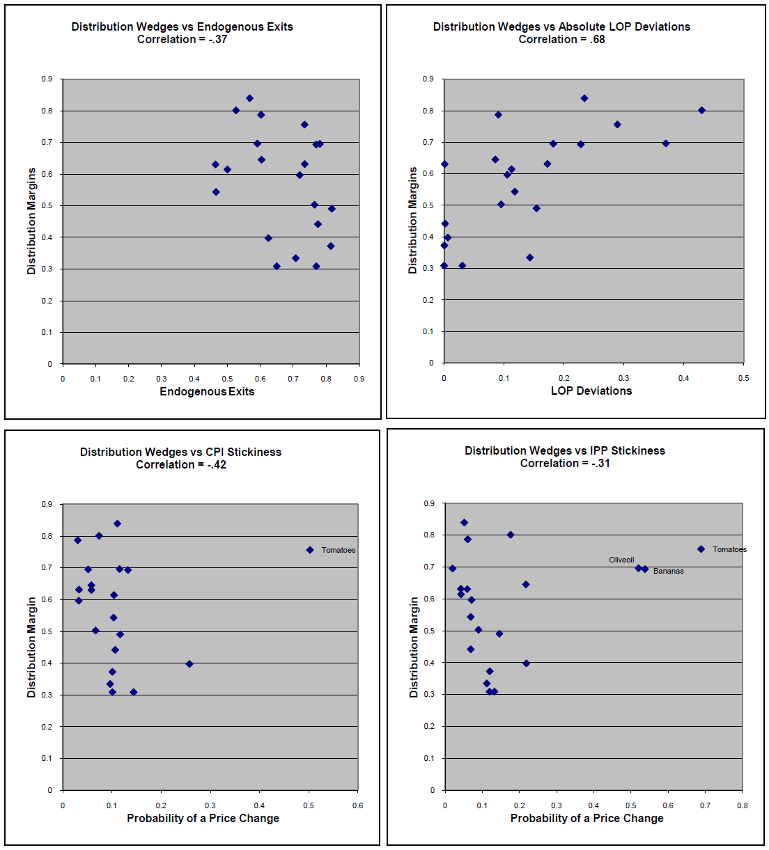
Appendix A: The Matching Procedure
As noted in the
text, in calculating distribution wedges ![]() we
compare the price of an item in the IPP database to that of a
matched item in the CPI database. We match items that are identical
in description. This appendix provides details on the criteria we
used to construct these matches. Naturally these criteria differed
across item categories. Each potential match was given a grade that
depended on how many of the criteria were met successfully. For
example, as described below, there were 5 criteria that had to be
met in order for there to be an " A Grade" match for that item:
product (e.g., vodka), proof (e.g., 80), size of the container
(e.g., 1 liter), brand, and country of origin. When a particular
criteria was not met, it was usually because that piece of
information was missing. In those cases when there was an obvious
mismatch on a criteria, e.g., brand of beer, an F grade was given.
In our empirical work we used only A grade and B grade matches.
we
compare the price of an item in the IPP database to that of a
matched item in the CPI database. We match items that are identical
in description. This appendix provides details on the criteria we
used to construct these matches. Naturally these criteria differed
across item categories. Each potential match was given a grade that
depended on how many of the criteria were met successfully. For
example, as described below, there were 5 criteria that had to be
met in order for there to be an " A Grade" match for that item:
product (e.g., vodka), proof (e.g., 80), size of the container
(e.g., 1 liter), brand, and country of origin. When a particular
criteria was not met, it was usually because that piece of
information was missing. In those cases when there was an obvious
mismatch on a criteria, e.g., brand of beer, an F grade was given.
In our empirical work we used only A grade and B grade matches.
Category: Alcohol
Grades: size, proof, BRAND, product, country of origin (mostly A's)
Category: Audioplayer
Grade Scale
A = Brand, model number + other character
B = Model number + other charact
C = partial model number +other characteristics
Category: Bananas
Match criteria: Brand, Country, Quality = A
B = a country (or brand) discrepancy from a mid sample switch in the CPI
C = country & brand tend to be off
Category: Beer
Grades: Brand, type, bottles vs. cans, country of origin
A = got them all
B = usually type and/or country of origin unknown in IPP
C = unknown type and container (usually in IPP) and unknown country of origin (usually in CPI)
Cans vs. bottles given an F
Discrepancy in container size given an F
Category: Calculator
Grades: Model Number and Brand (C tends to be off on a TI 83 "Plus" vs. no Plus)
Category: Cameras
If it matched on brand and model number gave it A;
If model number was missing but brand matched gave it a C;
If it matched model number but brand was missing gave it a B/C depending on how unique the model number seemed;
If brands were different gave it an F.
Category: Computer Accessories
A match on brand, model number, screen size/resolution
B match on screen size and model number +other characteristics
BC match on screen size, other characteristics and partial serial number (not enough info in IPP to know for sure)
Category: Drugs
Grade Scale
A = matches on brand, type and size of package and form of drug
B = believed to be an exact match but a major product characteristic is not listed in one of the descriptions
C = one major charateristic is off matches on brand but ipp size is half of what we want (C2) ; or (brand x) vs. (brand x max strength)
F = not a match
Category: Film
Criteria: Brand, Shutter Speed, Exposures
Number = Ratio of #rolls in CPI to IPP
Category: Mens Pants
Qualities: style number, brand, item description
A = style number, brand, and basic similarity of item description
B = often a downgrading from an A when the style number changed in the CPI sample
C = info just too spotty
F=clear country of origin contract (cpi=made in USA)
Category: Microwaves
Letter Grade: Brand, cubic feet, watts
A = all 3
B = brand info missing in IPP, cu ft and watt match
C = cu ft or watt info missing or off in IPP, brand info missing in IPP
F = watt and cu ft off or missing, brand info missing
Category: Miscellaneous Kitchen Appliances
Brand + model number = A.
Really long model number and other miscellaneous characteristics = A.
Model number match = B.
Anything else C or below.
Category: Oliveoil
A Matches on Brand, Type, Size and Bottle Type (plastic vs glass vs can)
B Matches on Brand, Type, Size
C Matches on Brand and Size
F Not a Match
Category: Phones
A: if it matched model/brand and serial OR serial was at least 7 digits and it matched other characteristics
B: matched serial only and serial was at least 4 digits
C: Matched serial and serial was 3 digits or les
F: matched nothing OR there was definitive evidence the two were different products.
Category: Stoves
Grades: mostly matched on serial numbers (Brand like George Foreman grill, specs like Bun Warmer)(not much else to go on other than proximity of the serial numbers)
Category: Tomatoes
We matched on brand, country of origin, type (cherry vs roma) and how it was grown (vine vs green house). If it hit brand and type and at least one of country and how it was grown (and no discrepancy in other) then it was an A. Otherwise if it type and at least one of country and how it was grown, then it was a B.
Category: Televisions
A matches on brand, model # and size at least
B matches on model# and size at least (and may have contradictory country of origin info)
C partial model # match and size
F not a match (wrong size etc.) or made in USA
Category: VCR
Qualities: Verbal description of item, model number, brand, country of origin
A = got everything essentially
B = model number and item description mostly, sometimes a brand match as well (still gave it B)
Category: Videocameras
Grades: mostly Bs = model number (good matches) and basic item description. Country of origin typically not in CPI, brand typically not in IPP
Category: Watch
A full serial number, country of origin/brand and other indetifiers
B serial number, country of origin + other indentifiers
C partial serial number, country of origin
F not a match
Category: Womens Pants
A identifiable brand, style number type of pants and country of origin
B usually no brand or country of origin
C incomplete style number, no brand
F made in USA or not a match.
Appendix to Table 1A and 2A Number of Observations (intra-company transfer prices excluded)
| Regular Price (CPI): cif | Regular Price (CPI): fob | Sale price (CPI): cif | Sale price (CPI): fob | |
|---|---|---|---|---|
| All items | 6054 | 14,090 | 1018 | 3316 |
| Alcoholic beverages | 2959 | 1108 | 660 | 166 |
| Audio players | 150 | 290 | 23 | 58 |
| Bananas | --- | 3482 | --- | 793 |
| Beer | 1509 | 3155 | 148 | 463 |
| Calculators | --- | 214 | --- | 19 |
| Cameras | --- | 199 | --- | 39 |
| Computer accessories | 20 | 110 | --- | 8 |
| Drugs | 7 | 89 | --- | --- |
| Film | 581 | 114 | 42 | --- |
| Men’s pants | --- | 128 | --- | 328 |
| Microwave ovens | --- | 126 | --- | 81 |
| Kitchen equip. (misc.) | --- | 157 | --- | 42 |
| Olive oil | --- | 170 | --- | 58 |
| Telephones | 65 | 341 | --- | 41 |
| Stoves | 82 | 246 | 29 | 71 |
| Tomatoes | 513 | 2231 | 62 | 544 |
| Televisions | 105 | 820 | 22 | 308 |
| VCRs | 56 | 633 | 29 | 153 |
| Video cameras | 7 | 206 | --- | 37 |
| Watches | --- | 134 | --- | 60 |
| Women’s pants | --- | 103 | --- | 35 |
Appendix to Table 1A and 2A Number of Observations (intra-company transfer prices only)
| Regular Price (CPI): cif | Regular Price (CPI): fob | Sale price (CPI): cif | Sale price (CPI): fob | |
|---|---|---|---|---|
| All items | 546 | 6210 | 173 | 1259 |
| Alcoholic beverages | 230 | 7 | 92 | --- |
| Audio players | 172 | 130 | 34 | 9 |
| Bananas | --- | 3447 | --- | 573 |
| Beer | --- | 122 | --- | 14 |
| Calculators | --- | 36 | --- | --- |
| Cameras | --- | 299 | --- | 46 |
| Computer accessories | --- | 30 | --- | 14 |
| Drugs | --- | 51 | --- | --- |
| Film | --- | 21 | --- | --- |
| Men’s pants | 12 | 149 | --- | 96 |
| Microwave ovens | --- | 10 | --- | 7 |
| Kitchen equip. (misc.) | --- | 171 | --- | --- |
| Olive oil | --- | 69 | --- | 12 |
| Telephones | --- | 226 | --- | 18 |
| Stoves | 76 | 14 | 21 | --- |
| Tomatoes | 6 | 10 | --- | --- |
| Televisions | 18 | 797 | 6 | 287 |
| VCRs | --- | 283 | --- | 72 |
| Video cameras | --- | 266 | --- | 93 |
| Watches | --- | 49 | --- | --- |
| Women’s pants | 27 | 10 | 20 | --- |
Footnotes
1. We thank Ariel Burstein and Linda
Goldberg for comments and Craig Brown, Rob McClelland, Daryl
Slusher, and Rozi Ulics, for their generous assistance. The views
in this paper are solely the responsibility of the authors and
should not be interpreted as reflecting the views of the Board of
Governors of the Federal Reserve System or of any other person
associated with the Federal Reserve System.
Return to text
2. Specfically, we follow the previous
literature (Burstein, Neves, and Rebelo 2003) and refer to the
distrution wedge as
![]() Return
to text
Return
to text
3. The issue is further confused by the fact that Engel's paper focuses on the real exchange rate of the U.S. and other large, developed economies whereas Burstein, Neves and Rebelo (BER) focus on the real exchange rate between the U.S. and emerging economies. There is reason to believe that this difference underlies some their diverging results. For instance, BER find that pass-through into dock prices for Argentina is almost 100% whereas Gopinath, Itshoki and Rigobon find that the corresponding figure for the U.S. is closer to 10%. Return to text
4. In Devereux, Engel and Tille (2003) the modeling was quite simple and designed solely to have two different prices, one for domestic consumers and one for exports. In their set-up, retailers did not use any resources such as labor. In the Corsetti, Dedola and Leduc frameworks, retailers use labor, so domestic factor costs matter for the consumer price of imported goods. In addition the absence of substitutability between labor in retail and in the imported good makes the retail price of the imported good a linear bundle of the imported good and local labor. As a result the foreign exporter faces a non-constant elasticity of demand, leading to several interesting findings, such as limited exchange rate pass-through even with flexible prices. Return to text
5. In their example complete pass-through would be 100% pass through. Local costs at the wholesale level lower pass-through to 50%. Variable markups at the wholesale level lower the pass-trhough percent to 18%. (or a 32% markup varation) close to what is observed in the data. Return to text
6. Hence, in the absence of other distortions, these production units earn zero profits in equilibrium. Return to text
7. Alternatively, one could consider the
case where a wholesaler purchases the item from an overseas
manufacturer at price ![]() , it requires
, it requires ![]() total distirbution costs to bring the item to retail
and
total distirbution costs to bring the item to retail
and ![]() is the total markup of the wholesaler and
the retailer. Return to text
is the total markup of the wholesaler and
the retailer. Return to text
8. Note that we are measuring the markup relative to the retail price, where traditionally the markup is measured relative to marginal cost. Thus our assumption that the markup relative to the retail price is a (significant) lower bound the the conventionally measured markup. Return to text
9. See Goldberg and Hellerstein (2008) Table 13 column 2. Return to text
10. Various authors report wedges in different ways. With the formula above the wedge is bounded by zero (when CPI price is greater than IPP) and unity. It has the intuitive interpretation as the fraction of the retail price, which consumers do observe, that is accounted for by transportation costs, overhead, retailer profit, etc. Return to text
11. This is relevant for the matching procedure but not the alternative procedure where we calculate weighted-average price levels for ELI categories. Under the latter we do not utilize such information as we are trying to use prices of as many items as possible, irrespective of whether the database contains specific information on the item. Return to text
12. Remember, they make assumptions so that the distribution margin is equal to the distribution cost. Return to text
13. We were able to construct reliable estimates of weighted-average price levels for only about half of the item categories used in the matching procedure. This was due to data limitations. Particularly constraining was getting information on whether a particular CPI item was produced in the United States or abroad. Return to text
14. There are noticeable jumps in the
![]() values in the final year, 2007, which
runs only through the month of July. We thus await an updating of
the data and decomposition results before putting too much stock in
these jumps. Return to text
values in the final year, 2007, which
runs only through the month of July. We thus await an updating of
the data and decomposition results before putting too much stock in
these jumps. Return to text
15. In any given year, about one-fifth to one-fourth of the items exit the sample " endogenously" in this way. This figure has remained fairly constant over time. Somewhat to our surprise, there is not a lot of cross-country variation when we count endogenous exits by country of origin of the imported item. Return to text
16. With the outliers, the correlation is essentially zero. Note that this negative relationship is consistent with the theorectical and empirical work presented in Gopinath and Itshoki (2008b). Return to text
17. This is the prototype regression found in the literature on exchange rate pass-through. Goldberg and Campa, (2006) provide details. Return to text
18. With apologies to Emi and Jon. Return to text
This version is optimized for use by screen readers. Descriptions for all mathematical expressions are provided in LaTex format. A printable pdf version is available. Return to text