Skip to: [Printable Version (PDF)]

Board of Governors of the Federal Reserve System
International Finance Discussion Papers
Number 1054, August 2012 --- Screen Reader Version*

Commodity Price Movements in a General Equilibrium Model of Storage

David M. Arseneau and Sylvain Leduc

NOTE: International Finance Discussion Papers are preliminary materials circulated to stimulate discussion and critical comment. References in publications to International Finance Discussion Papers (other than an acknowledgment that the writer has had access to unpublished material) should be cleared with the author or authors. Recent IFDPs are available on the Web at http://www.federalreserve.gov/pubs/ifdp/. This paper can be downloaded without charge from the Social Science Research Network electronic library at http://www.ssrn.com/.

Abstract:

We embed the canonical rational expectations competitive storage model into a general equilibrium framework thereby allowing the non-linear commodity price dynamics implied by the competitive storage model to interact with the broader macroeconomy. Our main result is that the endogenous movement in interest rates implied under general equilibrium enhances the effects of competitive storage on commodity prices. Compared to a model in which the real interest rate is fixed, we find that storage in general equilibrium leads to more persistence in commodity prices and somewhat lower volatility. Moreover, the frequency of stockouts is lower in general equilibrium. A key mechanism driving this result is a link between the ability of the household to smooth consumption over time and the level of storage in the stochasic equilibrium. Finally, the model is used to examine the macroeconomic effects of both biofuel subsidies for ethanol producers and, seperately, subsidies designed to insulate households from high food prices.

Keywords: Commodity prices, storage, general equilibrium, nonlinearity

JEL classification: E20, E31, Q11

1  Introduction

In the past few years commodity prices have experienced large fluctuations that have led policymakers and academics to reconsider the sources of price movements in commodity markets. The all-time high reached by oil prices at the onset of the global financial crisis in the spring of 2008 triggered congressional hearings in the United States about the role of speculation and financial markets in general as factors behind the increase in the price of oil and other commodity prices. Ultimately, this led the U.S. Commodity Futures Trading Commission to impose new rules limiting the size of positions in futures and swap markets in food, energy, and metals, as part of the broader Dodd-Frank financial reform.

However, movements in commodity prices are also closely tied to changes in world economic activity, as Figure 1 highlights. Commodity prices declined sharply in the fall of 2008, as the U.S. financial crisis intensified and spread around the world, halting global growth. They bottomed out early in 2009 and have since been on an upward trend as world economic activity has recovered, driven largely by relatively fast growth in emerging market economies. Clearly, fundamental factors play a major role in determining prices in commodity markets.¹ As emphasized recently by the Food and Agriculture Organization of the United Nations, traditional sources for food price variability like supply shortfalls combined with low levels of stocks are important factors behind the recent fluctuations in many food prices. The FAO reports that stocks of cereals, for instance, fell sharply in 2006 and reached an historic low in 2008, making it more difficult to draw down stocks to smooth out the effects of supply shortfalls or demand increases on prices. Similarly, stocks-to-use ratio for copper, aluminum, and other base metals have also been below historical averages for much of the 2005-2010 period (see, for instance, the World Economic Outlook (2011)).

In this paper, we reconsider the role of variations in stocks and changes in supply and demand as drivers of commodity prices. Our approach builds on the seminal work of Williams and Wright (1991) and Deaton and Laroque (1992, 1995, 1996) who looked at these issues using partial equilibrium models of commodity markets in which consumers, producers, and storers interact and that interaction endogenously determines commodity prices. In particular, risk neutral storage agents (whom we will hereafter refer to as speculators) decide whether to sell the commodity immediately or store it to sell it in the future depending on their expectations of future prices in relation with current spot prices and the costs of storage. One appealing aspect of these models is their ability to generate relatively volatile commodity prices that experience occasional spikes and are fairly persistent, even though the shocks underlying the model are iid.

We add to this literature by embedding storage in a relatively standard DSGE model often used to study the effects of oil-price increases on the economy (see, for instance, Kim and Loungani (1992)). However, in contrast to many papers in that literature, the price of commodities is endogenously determined in our model.² Households in our economy derive utility from consuming a final good produced by firms using labor, commodities, and a fix amount of capital. Households also consume commodities directly and supply labor to firms. As in Williams and Wright (1991) and Deaton and Laroque (1992), the model also includes risk neutral speculators who buy and sell commodities. However, in our framework the decision whether to store or not is directly influenced by movements in the real interest rate, which are determined endogenously.

We first show that the interaction between storage and interest rates in general equilibrium enhances the effects of competitive storage on commodity prices. Compared to a model in which the real interest rate is fixed, we find that storage in general equilibrium leads to more persistence in commodity prices. These results reflect two factors. First, movements in interest rates amplify the movement of storage in response to shocks. For instance, following a positive supply shock that raises consumption, the real interest rate declines leading to higher stocks as the opportunity cost of storage declines. Second, speculators hold more stocks in equilibrium thereby reducing the probability of stock outs and bringing about smoother and more persistent movements in spot as well as futures commodity prices as compared to a partial equilibrium model. Although commodity prices in the model remain less persistent than their empirical counterparts, this finding is nonetheless important since Deaton and Laroque (1992) find that the standard partial equilibrium competitive storage model fails to generate enough price persistence to be in line with the data.

Overall, the real interest rate in our model moves in ways that heightens the beneficial effects of speculation and storage on the economy and accentuates the effects on commodity prices in particular. This finding contrasts with some other results in the literature on models with explicit nonlinear constraints, such as that on lumpy investment under nonconvex adjustment costs. For instance, Thomas (2002) finds that the aggregate effects of lumpy investment are negligible in general equilibrium, as households preferences for smooth consumption profiles offsets the effects of lumpy investment at the plant level. In our model, the exact opposite occurs: Households' desire to smooth consumption implies movements in interest rates that amplify the movements in storage.

One advantage of using our general equilibrium framework is the ability to capture feedback effects brought about by changes in economic policy using a framework that is immune to the Lucas critique. In the last part of the paper, we exploit this feature of the model by examining two policy experiments. First, we consider the impact of biofuel (ethanol) subsidies in the United States as a source of high food (corn) prices. Legislation adopted in 2004 gives U.S. ethanol producers a $0.45 tax credit per gallon of ethanol produced on top of an existing $0.54 per gallon tariff on imports, among others. This policy change is often suggested as having contributed to the run down in global commodity stocks of corn over this period, possibly helping to increase food prices as a result. However, our model predicts a modest increase of 8 percent in food prices as a result of the biofuel subsidies. While our model is very stylized and abstracts from many realistic features of international commodity markets, we note that this result is in line with the findings of Babcock and Fabiosa (2011) derived from a large partial equilibrium model of the U.S. corn market.

Next, we examine the impact of introducing subsidies to mitigate the effects of high commodity prices on the economy, a policy followed by many countries during the food crisis of 2006-'08 to support households food consumption and to help firms pay for higher input prices. During the crisis, the cost of these subsidy programs rose substantially in many emerging markets and developing countries, costing in some instances as much as 5 percent of GDP or more (see IMF (2008)). Our model suggests that while the fiscal cost associated with these policies is high, the gains in terms of lower prices and higher output are fairly modest.

For some countries like Ecuador, Egypt, or Venezuela, the subsidy programs were very expensive, costing more than 5 percent of GDP. Food subsidies were also prevalent, with 28 countries reporting having such programs. As with fuel price subsidy programs, food price subsidy programs tend to be fairly costly as they are generally universal, i.e., they apply to anyone buying food products. Overall, the fiscal measures introduced to deal with the 2007-2008 crisis had a median price tag 0.6 percent of GDP, with roughly one-fifth of the countries surveyed by the IMF reporting a fiscal cost exceeding 1 percent of GDP.

To our knowledge, our paper is the first to examine the effects of competitive storage in general equilibrium. In addition to the early work in this literature mentioned above, our work complements to recent paper by Cafiero et al (2009) who reconsider the model of Deaton and Laroque (1992, 1995) using more precise numerical methods and show it to be important for the properties of the commodity price series simulated from the model. In addition, our work is also related to Ng and Ruge-Murcia (2000) and Miao, Wu, and Funke (2011), both of which introduce additional features in the competitive storage model to address the Deaton and Laroque criticism by improving its match with the data. Ng and Ruge-Murcia (2000) examine the ability of production lags, multiperiod contracts, and a convenience yield to generate increased persistence in commodity prices. To put our results in context, we find that the general equilibrium stucture of our model introduces a similar degree of persistence as any one of these mechanisms taken seperately. Similarly, Miao, Wu, and Funke (2011) adds shocks to the trends of output and demand to generate increased price persistence. Closer to our approach, these authors also consider shocks to the real interest rate, which leads to increased volatility in commodity prices. The overall sparsity of work in this area likely owes to the inherent nonlinearity of the model. Following Williams and Wright (1992), we numerically solve for the model's decision rules using polynomial approximation of the speculator's expectations of future commodity prices and households' expectations of future marginal utility.

The remainder of the paper is organized as follows. We present the competitive storage model in the next section, with a description of households' behavior, the firm's problem, and a discussion of the speculator. Following a brief description of the model's parameterization, Section 3 presents our results detailing the general equilibrium effects of storage. We then examine the impact of imposing subsidies to mitigate the negative effects of high commodity prices and the role of biofuel subsidies in generating high food prices. Finally, section 5 concludes.

2  The Model

We embed the canonical rational expectations storage model--as presented in Williams and Wright (1991), for example--into a general equilibrium macroeconomic framework. The model consists of households that make a static optimal labor supply decision as well as an intertemporal optimal savings decision, and a production sector. The production side of the model is divided into a final goods sector and a primary commodity sector. The final goods producing firm uses labor, capital, and the primary commodity as inputs into the production of a final good that is sold to and consumed by households. The primary commodity sector consists of both producers (farmers or mining companies, for example) as well as a risk neutral speculator (grain elevators or inventory storage facilities, more generally). As is typical in the rational expectations storage literature, the speculator exists to smooth volatility in the primary commodity sector.

2.1  Households

The household's utility function is defined over consumption of a final good, $c_{t}$, hours worked, $n_{t},$ and the consumption of a primary commodity, $q_{H,t},$ such as food, for example.

$$U_{t}=\sum_{t=0}^{\infty}\beta^{t}\left( \log c_{t}+\chi\log(1-n_{t})+\log q_{H,t}\right)$$ (1)

We assume that households can purchase state-contingent bonds, denoted $b_{t+1},$ so that asset markets are complete. The household chooses sequences of $c_{t},$ $n_{t},$ $q_{H,t},$ and $b_{t+1}$ to maximize (1) subject to an infinite sequence of flow budget constraints, given by:

$$c_{t}+\int p_{b,t+1}b_{t+1}=w_{t}n_{t}+b_{t}+p_{t}q_{H,t}^{{}}$$ (2)

where: $p_{b,t+1}$ is the price of the state-contingent bond that pays one unit of the final consumption good in a particular state of nature in time $t+1$; $w_{t}$ is the real wage; and $p_{t}$ is the relative price of the primary commodity.

The household efficiency conditions are as follows:

$$\frac{\chi c_{t}}{1-n_{t}}=w_{t}$$ (3)

$$\frac{1}{c_{t}}=\beta E_{t}\left[ \frac{1}{p_{b,t+1}}\frac{1}{c_{t+1}}\right]$$ (4)

$$c_{t}q_{H,t}^{-\sigma}=p_{t}$$ (5)

Equation (3) is standard and defines the household's optimal labor supply condition. Similarly, equation (4) is a standard consumption Euler equation pinning down the household's optimal saving decision. Note that we can use equation (4) to define the stochastic discount factor $E_{t}\left[ \Xi_{t+1\vert t}\right] =\beta E_{t}\left[ \frac{c_{t}}{c_{t+1} }\right] .$ Finally, equation(5) pins down the optimal household demand for the primary commodity by equating the marginal rate of substitution between the commodity and the final consumption good to the relative price of the commodity expressed in units of the final consumption good.

2.2  Production

The production side of the model can be thought of as having two sectors: a final goods sector and a primary commodity sector. We describe each in turn below.

2.2.1  The Final Goods Sector

The final good is produced using three inputs into production: labor, capital, and a primary commodity. Production of the final good is given by:

$$y_{t}=z_{t}n_{t}^{\gamma}\left( \left( 1-\omega\right) k_{t}^{\alpha }+\omega q_{I,t}^{\alpha}\right) ^{\frac{1-\gamma}{\alpha}}$$ (6)

where: $z_{t}$ is an aggregate productivity shock and $q_{I,t}^{{}}$ is the industrial usage of the commodity in production of the final good. For simplicity, we assume a fixed capital stock, so that $k_{t}^{{}}=\overline {k}.$

The final goods producing firm's profit function is

$$\Pi_{t}^{F}=\sum_{t=0}^{\infty}\left\{ \Xi_{t\vert}\left( y_{t}-w_{t} n_{t}-r_{t}^{k}\overline{k}-p_{t}q_{I,t}^{{}}\right) \right\}$$ (7)

where: $\Xi_{t\vert}$ is the period-0 value to the representative household of period-t goods that is used by the firm, which is ultimatly owned by households, to discount profits.

The firm's efficiency conditions are given by:

$$\gamma y_{t}\frac{1}{h_{t}}=w_{t}$$ (8)

$$\frac{\left( 1-\gamma\right) y_{t}\omega q_{I,t}^{\alpha-1}}{\left( 1-\omega\right) \overline{k}^{\alpha}+\omega q_{I,t}^{\alpha}}=p_{t}$$ (9)

Equation 8 defines the firm's optimal labor demand. Equation 9 defines the firm's demand for industrial usage of the primary commodity by equating the marginal product of an additional unit of the commodity to the marginal price.

2.2.2  The Primary Commodity Sector

The primary commodity sector consists of two types of agents: (1.) a producer of the primary commodity; and (2.) a speculator.

Commodity Production

Production of the commodity occurs with a one period lag; that is, the commodity producer plans in period $t-1$ the amount that will be produced in period $t$. $\$In terms of notation, denote planned production for producer $i$ as $\overline{h}_{t}^{i}.$ $\$While planned production is fixed at the beginning of period $t,$ actual production, denoted $h_{t}^{i},$ is subject to a stochastic disturbance, so that $h_{t}^{i}=\overline{h}_{t}^{i}\left( 1+\nu_{t}\right) .$ In this sense, the lag implies that production can be thought of as completely inelastic within the period. An optimizing producer chooses planned production, $\overline{h}_{t}^{i}$, in period $t-1\,$to maximize expected future profits in period $t$. The commodity producer's problem is

$$\Pi_{t}^{P,i}=\sum_{t=0}^{\infty}\Xi_{t\vert}\left\{ E_{t-1}\left[ h_{t} ^{i}p_{t}\right] -H\left( \overline{h}_{t}^{i}\right) \right\}$$ (10)

where: $H^{i}\left( \overline{h}_{t}^{i}\right)$ is the total cost to producer $i$ of producing the planned $\overline{h}_{t}^{i}$ units of total output of the primary commodity. In turn, total primary commodity output is given by $\overline{h}_{t}^{i}=\overline{h}-\eta^{P}P_{t}^{r}$, where $\overline{h}$ is a constant; $P_{t}^{r}$ is defined as the commodity producer's incentive price, or equivalently the expected increase in revenue resulting from an increase in planned production by one unit; finally, $\eta^{P}$ is the elasticity of production with respect to the incentive price.

The first order condition for profit maximization on the part of the commodity producer is given by

$$\frac{\partial E_{t-1}\left[ h_{t}^{i}p_{t}\right] }{\partial\overline {h}_{t}^{i}}=\frac{\partial H^{i}\left( \overline{h}_{t}^{i}\right) }{\partial\overline{h}_{t}^{i}}\equiv P_{t}^{r}$$ (11)

which simply equates the expected marginal revenue of an additional unit of production of the commodity to the marginal cost of production. We follow Williams and Wright (1001) and define the anticipated marginal revenue of an additional unit of production as the producer's incentive price, $P_{t} ^{r}\equiv\frac{\partial E_{t-1}\left[ h_{t}^{i}p_{t}\right] }{\partial h_{t}^{i}}.$

The commodity producer must commit one period in advance to a certain target level of production, which is determined by the firm's best forecast of both the future price as well as future realizations of the shock. Once target production is determined, actual production is subject to random shocks. Intuitively, imagine that a farmer must plant a crop well in advance of the point in time in which the crop is actually harvested. Once the crop is planted in the ground, a number of factors could influence the ultimate yield of the harvest. Weather could be unusually bad, leading to actual production that is much lower than planned production. Alternatively, good weather can lead to actual production that is exceptionally high relative to planned production. Weather itself, however, is a purely stochastic element of production. In the case of mining, imagine that a mine has a target level for copper production and must commit to a certain level of capital and labor input in advance in order to achieve this target. But, once the capital and labor is in place, actual production is subject to disturbances such as flooding, electricity outages, and labor unrest. The inability of producers to adjust to these shocks implies that production completely inelastic within the period, but is free to adjust (with potentially varying degrees of price elasticity) over longer horizons. Therefore, this setup captures some of the properties of putty-clay production models (see, for instance, Wei (2003) for an application of the Gilchrist and Williams (2000)'s model to the oil sector).

Commodity Storage

In this model, demand adjusts instantaneously to shocks while production is essentially inelastic in the short run; as such, the commodity market will be very volatile. A rational speculator helps to smooth this volatility by holding the commodity from period to period. The speculator compares the marginal gain of selling the commodity today to the opportunity cost of holding the commodity until tomorrow and selling at the discounted futures price net of the cost of storage.

In terms of notation, let $s_{t}$ denote the amount of storage accumulated in period $t$ that will be carried over by the speculator into period $t+1$. Also, let $\kappa$ denote the per unit storage cost, so that the total cost of storage is given by $\kappa s_{t}.$

The commodity speculator chooses the optimal amount of storage $s_{t}$ to maximize discounted lifetime profits defined as

$$E_{t}\Pi_{t+1}^{S}=\sum_{t=0}^{\infty}\beta^{t}\frac{\lambda_{t}}{\lambda_{0} }\left( E_{t}\left[ p_{t+1}s_{t}\right] -p_{t}s_{t}-\eta s_{t}\right)$$ (12)

The profit maximizing first order condition is given by

$$E_{t}\frac{p_{t+1}}{1+r_{t}}-p_{t}-\kappa=0$$ (13)

where $r_{t}$ is the real interest rate defined by equation (4) above.

However, physical storage cannot be negative, so we introduce this non-negativity constraint to express the optimal storage rule in the following manner

$$p_{t}+\kappa-E_{t}\frac{p_{t+1}}{1+r_{t}} =0 s_{t}>0$$ (14)

$$p_{t}+\kappa-E_{t}\frac{p_{t+1}}{1+r_{t}} \geq0 s_{t}=0,$$

We can also define the rational futures price of the commodity as $F_{t+1\vert t}=E_{t}\left[ p_{t+1}\right]$. Intuitively, the storage rule says that as long as the spot price of the commodity today is higher than the discounted futures price net of the cost of storage then it is optimal to sell all the commodity promptly and store nothing today as a result. Alternatively, if the spot price is sufficiently low relative to the discounted futures price net of the cost of storage, the speculator will accumulate inventories with the goal of selling the commodity in the future at the higher price. The speculator accumulates inventories up until the point at which the intertemporal arbitrage condition holds so that the spot price today is exactly equal to the discounted expected futures price net of the cost of storage.

Define the availability of the commodity as actual production today plus storage brought into the period, so that $A_{t}\equiv h_{t}+s_{t-1}.$ Aggregate demand for the commodity is the sum of household and industrial demand, so that $q_{t}=q_{H,t}^{{}}+q_{I,t}^{{}}.$ $\$Note that by equations (5) and (9), we can express the price of the commodity through the inverse demand function,

$$p_{t}(q_{t}^{{}})=\frac{1}{2}\left( q_{H,t}^{{}}+q_{I,t}^{{}}\right) .$$ (15)

Finally, in order for the commodity market to clear, it must be that aggregate final demand for the commodity is equal to total availability period $t$ net of the demand for storage that is to be carried over into period $t+1.$

$$q_{t}^{{}}=h_{t}+s_{t-1}-s_{t}=A_{t}-s_{t}$$ (16)

2.3  Equilibrium

Taking as given the exogenous driving force, $\nu_{t}$, and the fixed capital stock, $\overline{k}$, the equilibrium of the model is a sequence of $\{y_{t},$ $c_{t},$ $n_{t},$ $q_{H,t}^{{}},$ $q_{I,t}^{{}},$ $\overline{h} _{t},$ $s_{t},$ $w_{t},$ $p_{t},$ $r_{t}\}$ that satisfy: the household optimally conditions, given by equations(3), (4), (5); the optimality conditions of the final goods producing firm, given by equations (8) and (9); the optimality condition of the commodity producer, given by equation (11); and the optimal storage condition , equation (14)

In addition, we have the inverse demand equation given by equation (15), the storage market clearing condition, given by equation (16), and the aggregate resource constraint, $c_{t}=y_{t}.$

3  Quantitative Analysis

In this section we first present the parameterization of the model used in the baseline analysis and then turn to the main results. We solve the model using nonlinear numerical methods. Specifically, we discretize the state space for supply shocks and initial storage and approximate the speculator's expectations of future commodity prices as well as the households' expectations of future marginal utilities using polynomials in the state variables. Appendix A offers more detail on the solution algorithm.

3.1  Parameterization

The baseline parameterization is summarized in Table 1. For the household utility function, we set the scale parameter over leisure such that $\chi=1$ and consider a coefficient of relative risk aversion of one, so that $\sigma=1$. The frequency of the model is meant to be quarterly, so we we calibrate the discount factor to 0.9924, implying an annual real interest rate of three percent in the nonstochastic steady state.

In the final goods production sector, we normalize the aggregate level of technology to one, so that $z=1.$ Labor's share of production in the final good is set to $\alpha=0.7.$ For the production of the intermediate good, we set the share of the primary commodity to a relatively small number, $\omega=0.1.$ The substitutability between capital and the primary commodity in the production of the intermediate good is set at $\alpha=10,$ which implicitly delivers a price elasticity of demand for the primary commodity of $\eta^{P}=1/(1-\alpha)=-0.1.$ Finally, the inelastic capital stock is fixed at $\overline{k}=0.1.$

In the primary commodity sector, we set the level of production in the non-stochastic steady state so that $\overline{h}=50.$ Production of the commodity is assumed to be perfectly inelastic, so that $\eta^{P}=0.$ Finally, we set the cost of storage to zero, so that $\kappa=0.$

The shock process for production of the primary commodity is calibrated so that $\nu_{t}\underset{iid}{\symbol{126}}N(0,\sigma_{\nu}^{2}),$ where $\sigma_{\nu}^{{}}=0.20,$ which is similar to that used in Williams and Wright (1991).

When solving the version of our model under partial equilibrium, we assume that the real interest is set to its nonstochastic value (0.77 percent, at a quarterly frequency), while we keep the values of the remaining parameters the same.

3.2  Main Results

In what follows, we present two sets of results for every exercise. The first set of results is for a standard partial equilibrium rational storage model similar to that found in the textbook treatment by Williams and Wright (1991) and used by Deaton and Laroque (1992, 1995, 1996). The second set of results comes from our full blown general equilibrium setup. A comparison of the two sets of results highlights (if and) how the general equilibrium structure of the model alters the main predictions of the standard model.

3.2.1  Decision Rules

Before presenting simulation results and impulse response functions, it is first instructive to look at characteristics of the decision rules for households, firms, and speculators that come out of each of the two model setups. To highlight the model's nonlinearity, we present those rules for both a positive and a negative supply shock. Moreover, to emphasize the general equilibrium effects in the model, we compare the decision rules under both partial and general equilibrium. Figures 2 and 3 report the results for the case of a positive and a negative supply shock, respectively, as a function of values of initial storage, $s_{t-1}$.

For a positive supply shock, Figure 2 shows that the speculator's decision rule for storage is upward sloping and steeper than what a 45 degree line would indicate for most values of $s_{t-1}$, so that storage increases following the shock. For our results below, it is also important to note that compared to the partial equilibrium version of our model, there is more storage under general equilibrium. Although the difference appears small in the figure, it has key implications for our simulated results reported below. Because of the endogeneity of the real interest rate, consumption under general equilibrium reacts less to a positive supply shock than when the interest rate is fixed, as movements in the real interest rate allow households to better smooth consumption over time. The relatively weak response of consumption more than offsets the stronger storage response, leaving total production of the commodity less sensitive to the shock in our general equilibrium framework as compared to the partial equilibrium model. As a result, the price reaction is also dampened under general equilibrium.

As shown in Figure 3, the decision rules for a negative supply shocks have characteristics that are, in general, similar to those in Figure 2. However, one noteworthy difference arises as a result of the nonlinearity of the competitive storage model. The charts in Figure 3 clearly highlight the presence of kinks in all decision rules for low values of storage. Since the speculator cannot borrow commodities from the future, there is less possibility to smooth out the effects of a negative supply shock when stocks are running low and, as a result, the decline in the supply of commodities is more pronounced. In turn, commodity prices increase more in this case and the decline in consumption is accentuated. In general, the effects of general equilibrium on the decision rule are similar to those in Figure 2.

The effects of storage on commodity prices and commodity supply can be seen from Figure 4, which reports a typical simulation from our model.³ A first feature of the commodity price series is the presence of occasional spikes, which occur following negative supply shocks and lead to stock outs. In these cases, the amount of commodities supplied to the market declines sharply. Another characteristic of the simulated commodity prices that come out of the model is the fact that they display autocorrelation despite the fact that the underlying supply shocks are iid. Because of the possibility to hold stocks, the effects of disturbances can be more easily spread over many periods, generating a propagation mechanism internal to the model.⁴

3.2.2  Spot and Futures Prices

As indicated in Tables 2 and 3, a high variance and autocorrelation are two salient attributes of commodity prices in the data. Table 2 simply reproduces some of the moments in Table 1 in Deaton and Laroque (1992) for annual commodity prices since 1919. As a complement, Table 3 shows the same statistics for copper, corn, wheat, and oil, using quarterly data starting in 1988, which we use to compare to our simulated data.⁵ In addition, Table 3 reports statistics for futures prices. Overall, the two tables indicate that commodity prices are very persistent, with autocorrelation ranging between 0.72 for Jute to 0.94 for bananas in Table 2 and between 0.68 and 0.86 in Table 3. This characteristic is also a property of commodity price futures. Moreover, in Table 3 we report the detrended volatility of commodity prices relative to the volatility of industrial production. For copper, corn, wheat, and oil, prices display a high volatility, with prices being more than 5 timesas volatile as production.

Using long simulations of 50,000 periods to approximate the stochastic steady state of the model, we examined the model's ability to generate properties of commodity prices in line with the statistics reported in Table 3. We find that storage under either partial or general equilibrium leads to significant volatility in spot and futures commodity prices, but still much less so than in the data. These prices are roughly 2.4 times as volatile as final goods output, about half its empircal counterpart. Moreover, Table 4 shows that storage in general equilibrium raises the persistence of spot commodity prices by about 25 percent compared with the partial equilibrium version of the model. In addition, we find that the probability of stockouts is roughly halved under general equilibrium, which is an important property of the model since the probability of stock outs is low empirically. Deaton and Laroque (1992) report estimates of the probability of stock outs to range from 1 percent for palm oil to 23 percent for sugar with an average estimate across all commodities of 10.4. Thus, in our model simulations moving from partial to general equilibrium reduces the frequency of stock outs from the upper range of Deaton and Laroque's estimates to something very close to the average of their estimates.

The increased autocorrelation of commodity prices under general equilibrium partly reflects the higher average level of stocks reported in Table 4. Because the level of stocks tends to be higher, the effects of supply shocks can be more easily spread out over many periods. The following section provides more intuition through an impulse response analysis.

3.2.3  Storage and the Real Interest Rate

The higher stocks in general equilibrium are an optimal response by speculators to movements in the real interest rate. To see this, consider the effect of positive supply shock in Figure 5. Consistent with the decision rules above, the figure indicates that following the shock, storage increases slightly more under general than partial equilibrium. This finding reflects the fact that, ceteris paribus, it is optimal for the speculator to store more when the opportunity cost of storage, the real interest rate, declines which, in general equilibrium, occurs in line with the household's optimal consumption path. The higher stocks in turn imply less increase in market supply and less downward movements in prices, which similarly tend to die off less rapidly than under partial equilibrium.

The importance of the mean levels of storage reported in Table 4 is accentuated when we consider the effects of a large negative supply shock, which we report in Figure 6. There the differences between the responses under general versus partial equilibrium are striking. Because stocks are lower under partial equilibrium, the negative supply shocks leads to a stock out and hence to a spike in the spot price and a sharp decline in consumption. Consistent with the decision rules above, once a stock out occurs, inventories are not build back up again. (In a stochastic simulation they would rise when the economy eventually experiences a sufficient number of positive supply shocks.) Because of the stockout, the futures price drop and stays constant at that lower level thereafter (Similarly, in a stochastic simulation the futures price will eventually rise in response to positive shocks).

In contrast, despite the fact that the higher opportunity cost of storage (via a higher real interest rate) increases the incentive to deplete stocks, the higher overall level of inventories in general equilibrium implies that this depletion does not cause a stock out. Overall, these effects imply that the economy under general equilibrium is better able to cope with a negative supply shock and, as a result, the impact on consumption and spot and futures prices are mitigated. Similar to the case of a positive supply shock, the declines in consumption and prices are propagated over multiple periods via the persistent decline in storage.

4  Policy Experiments

In this section, we use our framework to conduct policy experiments to better understand how interventions in the commodity market interact with the broader macroeconomy. We focus on two specific fiscal interventions that received considerable attention during the food and energy crisis that played out during the 2006-2008 period: biofuel subsidies in the United States and food and fuel subsidies in many emerging markets economies to mitigate the effects of high commodity prices.

The large increases in the real prices of many commodities over this period, which is illustrated in Figure 7, had many sources. Yet, the rapid rise in commodity prices over this period is often ascribed to a unique confluence events. First, robust demand stemming from unprecedented strength in global growth --driven in large part by the emerging market economies and China, in particular--over much of the preceeding decade ultimatly led to relatively low levels of stocks in the mid 2000s, compared to historic norms for many commodities. Second, a series of large and persistant negative supply shocks (the drought in Australia, India's rice export ban, the shutting-in of significant amounts of oil production in Venezuela and Iraq) occurred as stocks reached those very low levels.

The competitive storage model predicts that commodity prices are particulary responsive to adverse supply shocks at times when stocks are low. For instance, Figure 8 shows the ratios of world ending stocks to world consumption for three staple commodities, corn, rice, and wheat, since 1960. The drops in the stock-to-use ratios since the early 2000s were particularly dramatic for rice and corn, but a decrease is also noticeable for wheat. For rice and corn, one has to go back to the mid-1970s or the beginning of the1980s to see stock-to-use ratios as low as they were in 2007-2008. Moreover, stocks were also low for other commodites, like copper, aluminum, and other base metals more generally (see, the IMF World Economic Outlook (2011)).

The historical relationship between detrended stock-to-use ratios and detrended prices is reported in Figure 9 for wheat, rice, and corn. The figure shows a clear negative relationship for the three grain markets: prices tend to be higher when stocks are low. As pointed out by Dawe (2009), the recent declines in grains stock-to-use ratios have been largely driven by China's drawdown of its own stocks. However, as indicated in Figure 10, excluding China from the calculation has a minimal effect on the negative relationship between stock-to-use ratios and commodity prices.

In light of this, the increase in biofuel subsidies in the United States in 2004 to encourage ethanol production helped to artificially support demand and contributed to the run down in global commodity stocks of corn over this period, possibly helping to increase both the level and volatility of food prices. A common policy response by many emerging market economies during the food crisis was to implement or increase existing commodity price subsidies to insulate domestic consumers from higher and more volatile prices. These two policy interventions--biofuel subsidies to ethanol producers and food price subsidies to consumers--motivate the two policy experiments descibed in the following subsections.⁶

4.1  Biofuel Subsidies

The large increase in the real price of corn reported in Figure 6 occurred at the same time that corn-based ethanol production boomed in the United States (it became the largest ethanol producer in 2005), partly driven by changes in energy efficiency requirements and by the presence of subsidies and tariffs. Legislation adopted in 2004 gives U.S. ethanol producers a $0.45 tax credit per gallon of ethanol produced on top of an existing $0.54 per gallon tariff on imports, among others. This policy change is often suggested as a source of the runup in corn prices that started in 2005, since U.S. ethanol is mainly produced using corn.

To examine the effects of a production subsidy on commodity prices we use our model and think of the commodity produced as representing corn. In turn, we interpret the use of the commodity in the production function (6) as ethanol fuel. For simplicity, we assume that corn can be transformed one to one into ethanol. Introducing another sector that produces ethanol using corn would add realism to the exercise, but wouldn't change the gist of our results. We then assume that the use of "ethanol" in the production function is subsidized at rate $\tau_{q_{I},t}.$ Empirically, the $0.45 tax credit per gallon of ethanol produced averages roughly 25 percent of the price of ethanol between 2003 and 2006, which we use in our simulation (see, EIA (2007)). As before, we assume that the cost of the subsidy is financed by a labor income tax.

The effects of the subsidy can be clearly seen by looking at the model's decision rules under the presence of the production subsidy or without it. Figure 11 shows that, for a given level of stocks, introducing an ethanol subsidy raises the production of ethanol and its use in the production of the final good.⁷ The price of corn is driven higher as a result, and households respond by cutting their corn consumption. The effect of the subsidy on the consumption of the final good is more muted as the share of corn in the final good's production is relatively small.

Similarly, the increase in the price of corn brought about by the introduction of the subsidy is small in the figure. For any level of corn stocks, the subsidy increases the price of corn by roughly 6 percent following our largest supply contraction. This order of magnitude is also born out in a stochastic simulation exercise in which we simulate the model for 50,000 periods. In this case, we find that the subsidy raises the mean level of corn prices by about 7 percent.

While our model is clearly stylized and abstracts from many realistic features of the corn and ethanol markets, the effect of the subsidy on prices is very similar to that in Babcock and Fabiosa (2011) who use large static partial equilibrium model of the corn market. Studying the effects of ethanol subsidies on corn prices between 2005 and 2009, they find that it raised prices by roughly 8 percent. We view our approach as complementing their more detailed analyis of the corn market's structure and take from the two approaches that the effect of biofuel subsidies on corn prices is relatively small.

4.2  Food Price Subsidies

As discussed above, many countries pursued diverse policies to mitigate the economic and social impact of higher commodity prices, particularly the effects coming from large increases in food and oil prices. One popular strategy adopted was the introduction or the increase of already existing subsidies to firms and households. The IMF documents that fuel price subsidies increased substantially between 2006 and 2008 for at least 38 countries and that by the end of that period a total of 46 countries had subsidies in place (see IMF (2008)). For some countries like Ecuador, Egypt, or Venezuela, the subsidy programs were very expensive, costing more than 5 percent of GDP. Food subsidies were also prevalent, with 28 countries reporting having such programs. As with fuel price subsidy programs, food price subsidy programs tend to be fairly costly as they are generally universal, i.e., they apply to anyone buying food products. Overall, the fiscal measures introduced to deal with the 2007-2008 crisis had a median price tag 0.6 percent of GDP, with roughly one-fifth of the countries surveyed by the IMF reporting a fiscal cost exceeding 1 percent of GDP.

In this subsection we use our model to evaluate the effectiveness of using subsidies to insulate consumers from commodity price movements and to better understand the macroeconomic impact of such subsidies. We assume that the government subsidizes households' consumption of commodities and that it finances this expenditure with a labor income tax. To capture the fact that in many countries the subsidies tended to increase with the rise in commodity prices, we assume that the government subsidy follows the following process

$$\tau_{q_{H},t}=\overline{\tau}_{q_{H}}+\psi_{p}p_{t},$$

where $\overline{\tau}_{q_{H}}$ is the steady state level of the subsidy and $\psi_{p}$ captures the responsiveness of the subsidy to movements in the real price of commodities.⁸ We set $\overline{\tau}_{q_{H}}$ and $\psi_{p}$ so that the average cost of the subsidy is roughly 4 percent of output, so at the high end of the fiscal costs experienced by countries with such programs in 2007-2008.

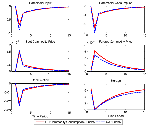
Figure 12 reports the movements in some variables of interest following a severe negative supply shock with and without subsidies. The charts show variables in deviations from steady state, with the exception of storage, which is shown in levels. The chart for storage shows that stocks are slightly higher under a subsidy. A stockout occurs following the shock with or without the subsidy, which causes commodity prices to initially spike. However, more stocks are released to the market when food consumption is subsidized (since the level of stocks is initially higher), and the market supply increases more and commodity prices less as a result. The introduction of the subsidy supports commodity and overall consumption, which decline less following the shock than when food consumption is not subsidized. In turn, firms' demand for commodities is slightly stronger, reflecting the relatively stringer demand for final goods

Overall, our results suggest that food price subsidies offer little bang for the buck in the sense that the overall impact of the commodity market is small given the large fiscal burden required to implement them in the first place.⁹

5  Conclusions

We embedded the canonical rational expectations competitive storage model into a general equilibrium framework. Using this model, we focus our attention on the way in which the broader macroeconomy interacts with the predictions of the partial equilibrium competitive storage model. To our knowledge, this is the first paper to undertake such an analysis. Our main result is that the interaction between storage and interest rates under general equilibrium enhances the effects of competitive storage on commodity prices. Compared to a model in which the real interest rate is fixed, we find that storage in general equilibrium leads to more persistence in commodity prices, but also to slightly less volatility. Moreover, the probability of stock outs is lower under general equilibrium. A key mechanism driving this result is a link between the ability of the household to smooth consumption over time and the level of storage in the stochastic equilibrium. In short, higher levels of storage are required for the household to be able to achieve a sufficiently smooth path for consumption over time.

A key advantage of our framework is the ability to conduct policy analysis in order to better understand the impact of commodity market policy interventions on the broader macroeconomy in an environment that is immune to the Lucas critique. To this end, we examine the impact of subsidies on commodity consumption at the intermediate goods producer level as observed in biofuel subsidies designed to encourage U.S. ethanol production, and at the household level as observed in practise in many emerging market economies during the food and fuel crisis of 2006-'08. On net, our results suggest that these subsidies do little to significantly alter commodity price dynamics and have only minor impacts on the broader macroeconomy. At the same time, they impose a significant fiscal burden on the governments that implement them.

Looking forward, there are a wide number of possible extensions that one could think of for this basic modeling framework. One that is of particular interest would be to introduce staggered price setting on the part of the final goods producing firm in order to open up a role for monetary policy over the business cycle. Such an extension could then be used to better understand how monetary policy interacts with commodity price dynamics. Another interesting extension might be to articulate the role of the exchange rate in commodity price dynamics in a small open economy version of the model.

References

Atkeson, A. and P.J. Kehoe, 1999, "Models of energy use: Putty-putty versus putty-clay," American Economic Review 89(4), 1028-1043.

Babcock, B.A. and J.F. Fabiosa, 2011, "The impact of ethanol and ethanol subsidies on corn prices: Revisiting history", Iowa State University, CARD Policy Brief 11-PB 5.

Bodenstein, M. and L. Guerrieri, 2011, "Oil efficiency, demand, and prices: a tale of ups and downs," Federal Reserve Board of Governors Working Paper 1031.

Cafieri, C., E.S.A. Bobenrieth, J.R.A. Bobenrieth, and B.D. Wright, 2011, "The empirical relevance of the competitive storage model," Journal of Econometrics, 162, 44-54.

Dawe, D., (2009), "The unimportance of `low' world grain stocks for recent wrold price increases," ESA Working Paper, 09-01, Rome, FAO.

Deaton, A., and G. Laroque, 1992, "On the behavior of commodity prices," Review of Economic Studies, 59(1), 1-23.

Deaton, A., and G. Laroque, 1995, "Estimating a nonlinear rational expectations commodity price model with unobservable state variables," Journal of Applied Econometrics, 10, S9-S40.

Deaton, A., and G. Laroque, 1996, "Competitive storage and commodity price dynamics," Journal of Political Economy, 104(5), 896-923.

FAO, 2009, "The state of aggricultural commodity markets,"

Gilchrist, S. and J. Williams, 2000, "Putty-clay and investment: A business cycle analysis," Journal of Political Economy, 108(5), 928-960.

Glick, R. and S. Leduc (forthcoming), "Central bank announcements of asset purchases and the impact on global financial and commodity markets," Journal of International Money and Finance.

IMF, 2008, "Food and fuel prices--Recent developments, macroeconomic impact, and policy responses," Washington, DC: International Monetary Fund.

IMF, 2011, "World Economic Outlook," Washington, DC: International Monetary Fund.

Kim, I.M. and P. Loungani, 1992, "The role of energy in real business cycle models," Journal of Monetary Economics, 29(2), 173-189.

Leduc, S. and K. Sill, 2004, "A quantitative analysis of oil-price shocks, systematic monetary policy, and economic downturns," Journal of Monetary Economics 51, 781-808.

Miao, Y., W. Wo, and N Funke, 2011, "Reviving the competitive storage model: A holistic approach to food commodity prices," IMF Working Paper WP/11/64.

Ng, S., and F. J. Ruge-Murcia, 2000, "Explaining the persistence of commodity prices," Computational Economics, 16, 149-171.

Thomas, J.K., 2002, "Is lumpy investment relevant for the business cycle?" Journal of Political Economy, 110(3), 508-534.

Wei, C., 2003, "Energy, the stock market, and the putty-clay investment model," American Economic Review, 93(1), 311-323.

Williams, J.C., and B. D. Wright, 1991, Storage and Commodity Markets, Cambridge University Press, Cambridge, U.K.

Wright, B. D., 2001, "The economics of grain price volatility," Applied Economic Perspectives and Policy, 33(1), 32-58.

A  Details on Model Solution

The optimal storage decision involves a nonlinear constraint; as such, we need to solve the model using nonlinear methods. Following Williams and Wright (1991), we use a polynomial approximation to link both the expected future price of the commodity, $E_{t}\left[ p_{t+1}\right]$, as well as expected future marginal utilities, $E_{t}\left[ \frac{1}{c_{t+1}}\right]$, to the current level of storage, $s_{t}$, the state variable in the model.¹⁰

In terms of notation, denote the polynomial linking expected future price to the level of storage today as $\psi^{p}(s_{t}).$ Similarly, denote the polynomial linking expected future marginal utilities to the level of storage today as $\psi^{c}(s_{t}).$ We assume a storage grid of size $N$ so that for all finite states the amount of storage taken out of any given period is denoted by the vector $\widetilde{s}_{t}=[s_{t}^{i=1},s_{t}^{i=2},\ldots ,s_{t}^{i=N}].$ $\$For the shock process, we approximate a continuous normal distribution with a discrete approximation with $M$ points, so that for all finite states the vector of all possible shocks is denoted by $\widetilde{\nu }_{t}=[\nu_{t}^{j=1},\nu_{t}^{j=2},\ldots,\nu_{t}^{j=M}].$

The goal of the solution algorithm is to find the coefficients for these two polynomials that are self replicating (ie, consistent with the rational expectations equilibrium). In practise, doing so requires six loops embedded within one another. Conditional on an initial guess for the coefficients of the polynomials $\psi_{0}^{p}(s_{t})$ and $\psi_{0}^{c}(s_{t}),$the algorithm takes the following general form:

Step 1.

Formulate initial guess for coefficients in optimal storage r

ule, $E_{t}\left[ p_{t+1}\right] =\psi^{s}(s_{t}).$

Step 2.

Formulate initial guess for coefficients in optimal savings function, $E_{t}\left[ \frac{1}{c_{t+1}}\right] =\psi^{c}(s_{t})$.

Step 3.

Formulate initial guess for planned production, $\overline{h},$ so that the vector of actual production for each realization of the shock is given by $h_{t}=(1+)\widetilde{\nu}_{t}.$

Step 4.

Conditional on each realization of the shock, for every level of storage available in period $t$ on the grid use MATLAB's non-linear equation solver to find: (1.) the optimal amount of storage, $s_{t+1}^{i,j}$, to take into period $t+1$; and (2.) the optimal amount of consumption, $c_{t}^{i,j}$, that satisfies the [private equilibrium] and, in the case of storage, also respects the non-negativity constraint.

Step 5.

For every level of storage available in period $t$ on the grid, calculate both the expected price, the expected marginal utility of consumption, and the producer's incentive price across all states of the shock. Using the producer's incentive price, calculate actual production, $h_{t},$ for every level of storage conditional on the distribution of the shock.

Step 6.

For every level of storage available in period $t$ on the grid, evaluate $\left\vert h_{t}-\overline{h}\right\vert <\varepsilon.$ If the convergence criteria is satisfied then we have found the optimal level of production and we go on to step 7; otherwise, we update the guess of $\overline{h}$ and the implied vector for actual production, $h_{t}$, and return to Step 4.

Step 7.

Regress $E_{t}\left[ \frac{1}{c_{t+1}}\right]$ across all levels of storage available in period $t$ on the grid and conditional on the shock distribution on storage, $s_{t}$, using the assumed third order polynomial to obtain the coefficient estimates in the vector $\widehat{\psi }_{{}}^{c}(s_{t})$. Evaluate $\left\vert \widehat{\psi}_{{}}^{c}(s_{t} )-\psi_{{}}^{c}(s_{t})\right\vert <\varepsilon.$ If the convergence criteria is satisfied then we have found the self-replicating polynomial expressing $E_{t}\left[ c_{t+1}\right]$ as a function of $s_{t}$ and we proceed to step 8; otherwise, we update the guess for the coefficients in the polynomial $\psi_{0}^{c}(s_{t})$ and return to Step 3.

Step 8.

Regress $E_{t}\left[ p_{t+1}\right]$ across all levels of storage available in period $t$ on the grid and conditional on the shock distribution on storage, $s_{t}$, using the assumed third order polynomial to obtain the coefficient estimates in the vector $\widehat{\psi}_{{}}^{p} (s_{t})$. Evaluate $\left\vert \widehat{\psi}_{{}}^{p}(s_{t})-\psi_{{}} ^{p}(s_{t})\right\vert <\varepsilon.$ If the convergence criteria is satisfied then we have found the self-replicating polynomial expressing $E_{t}\left[ p_{t+1}\right]$ as a function of $s_{t}$ and, hence, the rational expectations equilibrium; otherwise, update the guess for the polynominal $\psi_{0}^{p}(s_{t})$ and return to Step 2.

In our implementation, we use a third-order polynominal with the properites, $\partial\psi(s_{t})/\partial s_{t}<0$ and $\partial^{2}\psi(s_{t})/\partial s_{t}^{2}\geq0$, for both $\psi^{p}(s_{t})$ and $\psi^{c}(s_{t}),.$a storage grid with 60 points, and a convergence criteria of $\varepsilon=1e^{-12} .$

Table 1a: Model Parameterization (Household Utility)

Parameter	Value	Description
$\chi$	1	Scale parameter governing utility over leisure
$\sigma$	1	Curvature parameter for consumption of the primary commodiey
$\beta$	0.99	Household discount factor

Table 1b: Model Parameterization (Final Goods Sector)

Parameter	Value	Description
$z$	1	Steady state level of technology in final goods production
$\gamma$	0.7	Labor's share in final goods production
$\omega$	0.1	Share of primary commodity in production of the intermediate good
$\alpha$	10	Substitutability between capital and primary commodity in production of intermediate good
$\overline{k}$	0.1	Fixed capital stock

Table 1c: Model Parameterization (Primary Commodity Sector)

Parameter	Value	Description
$\overline{h}$	50	Level of production in the non-stochastic steady state
$\eta^{P}$	0	Elasticity of production with respect to price
$\kappa$	0	Cost of storage

Table 2: Properties of Commodity Prices: Annual Data since 1919$^{a}\bigskip$

Commodity	Autocorrelation
Bananas	0.92
Cocoa	0.84
Coffee	0.80
Copper	0.85
Cotton	0.89
Jute	0.72
Maize	0.76
Palm	0.73
Rice	0.84
Sugar	0.63
Tea	0.81
Tin	0.89
Wheat	0.87
Median$^{b}$	0.84

$^{a}$The data is from Deaton and Larocque (1992). We use data from 1919 onward so that we can use industrial production to scale the volatility of commodity prices.

Table 3: Properties of Spot and Futures Commodity Prices: Quarterly Data since 1988$^{a}\bigskip$

Commodity	Spot Prices: Autocorrelation	Spot Prices: Relative Volatility	3-Month Futures Prices: Autocorrelation	3-Month Futures Prices: Relative Volatility
Copper	0.77	6.89	0.78	5.08
Corn	0.68	6.48	0.68	6.71
Oil	0.68	6.71	0.69	6.09
Wheat	0.77	7.22	0.77	5.44

$^{a}$The data is taken from Haver Analytics. Spot and futures prices are detrended using the HP filter. Volatility is reported relative to detrended U.S. Industrial Production.

Table 4: Simulated Moments Under General and Partial Equilibrium

	General Equilibrium	Partial Equilibrium
Autocorrelation: Spot Commodity Price	0.54	0.43
Autocorrelation: Futures Prices	0.78	0.74
Relative Volatility: Spot Commodity Price	2.33	2.33
Relative Volatility: Futures Prices	1.4	1.1
Mean Storage	8	6
Probability of Stock outs	11.7	19.3

Figure 1: Commodity Prices and World Industrial Production

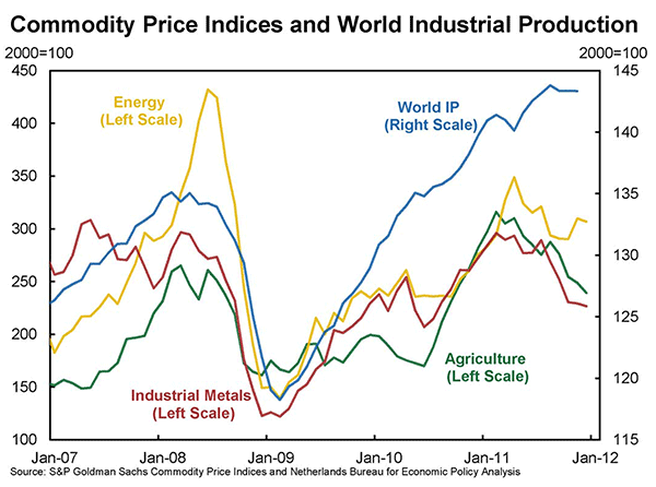
Figure 2: Decision Rules Conditional on a Positive Shock to Commodity Production, Partial Versus General Equilibrium

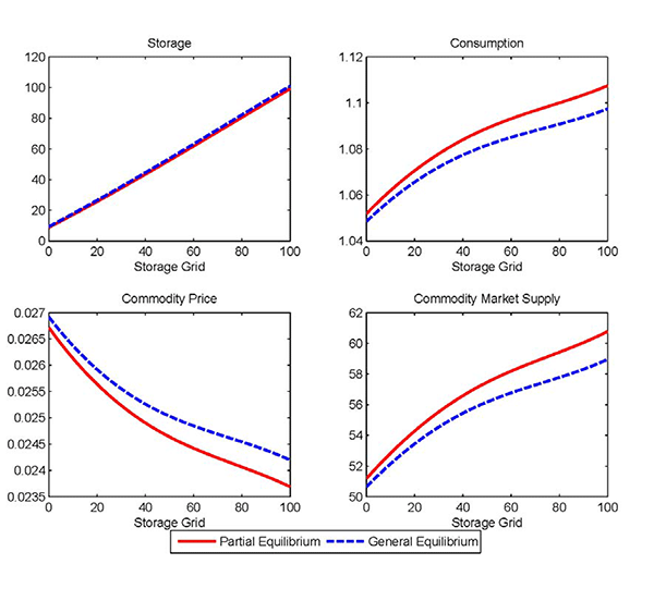
Figure 3: Decision Rules Conditional on a Negative Shock to Commodity Production, Partial Versus General Equilibrium

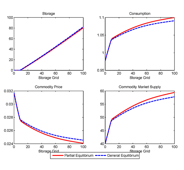
Figure 4: Model Simulated Data

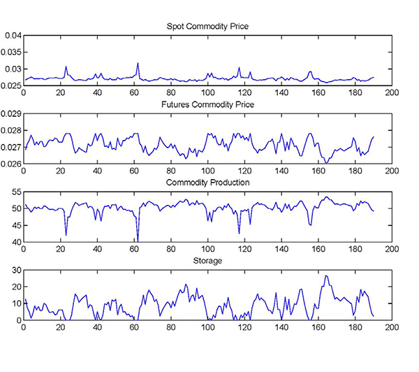
Figure 5: Impulse response functions to a positive shock to commodity production, general versus partial equilibrium. IRFs are calculated by first simulating the model with a series of draws of zero shocks for 100 periods. We then introduce a single shock and let the model gradually return to the stochastic steady state conditional on the series of draws of zero shocks.

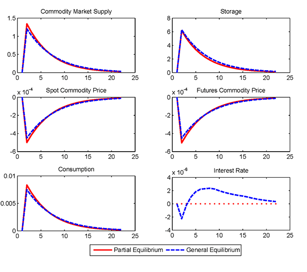
Figure 6: Impulse response functions (IRFs) to a negative shock to commodity production, general versus partial equilibrium. IRFs are calculated by first simulating the model with a series of draws of zero shocks for 100 periods. We then introduce a single shock and let the model gradually return to the stochastic steady state conditional on the series of draws of zero shocks.

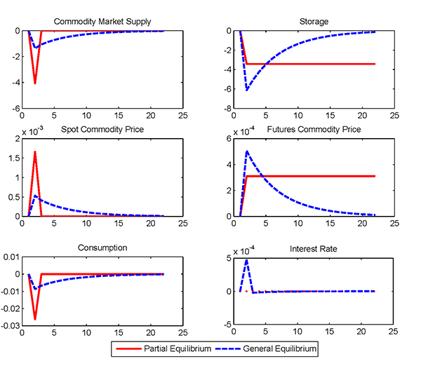
Figure 7: Real Commodity Prices, 1960-2010

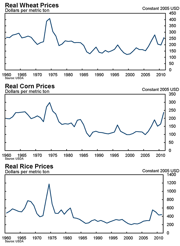
Figure 8: Global Stocks to Consumption Ratio, 1960-2010

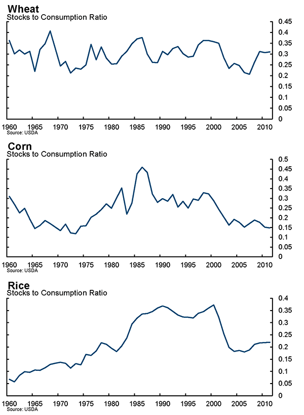
Figure 9: Scatter plot of real commodity price and stock-to-consumption ratio, percent deviation from HP filtered trend.

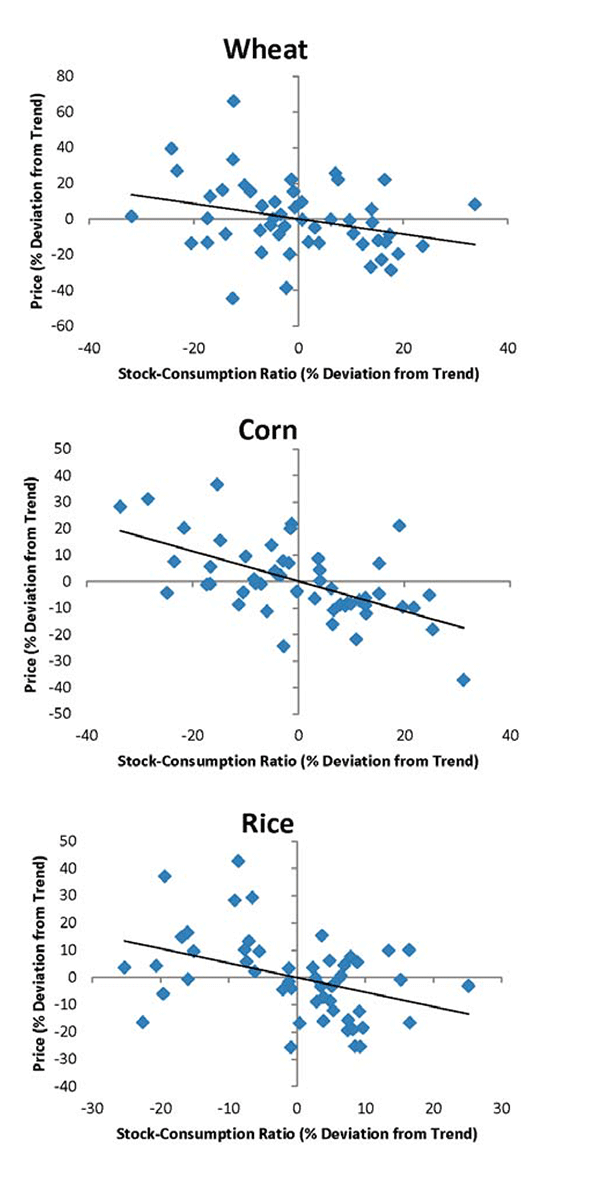
Figure 10: Scatter plot of real commodity price and stock-to-consumption ratio (ex. China), percent deviation from HP filtered trend.

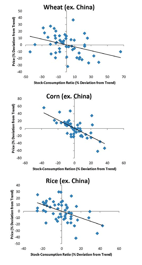
Figure 11: Decision rules conditional on a negative shock to commodity production, with and without input subsidy.

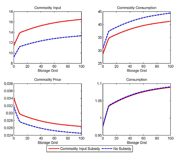
Figure 12: Impulse response functions (IRFs) to a negative shock to commodity production, with and without consumption subsidy. IRFs are calculated by first simulating the model with a series of draws of zero shocks for 100 periods. We then introduce a single shock and let the model gradually return to the stochastic steady state conditional on the series of draws of zero shocks.

Footnotes

1.  Unconventional monetary policy since the onset of the crisis has also lead to the criticism that sustained low interest rates are fueling the rise in oil prices. Using a standard New Keynesian open economy model, Bodenstein and Guerrieri (2011) find that changes in monetary policy have little effects on oil prices. See also the analysis of the effects of large-scale asset purchases by the Federal Reserve on commodity prices in Glick and Leduc (forthcoming). Return to text

2.  See, for instance, Atkeson and Kehoe (1999), Leduc and Sill (2004), or Wei (2003). Return to text

3.  For expositional purposes, we use a relatively short simulation length of 100 model periods. Return to text

4.  This property of the storage model is lacking in the typical real business cycle model and relatively weak in the financial accelerator model. See, for instance, Cogley and Nason (1995) and Carlstrom and Fuerst (1998). Return to text

5.  The difference in sampling period is driven by data availability. Commodity prices at the quarterly frequency--the frequency at which our model is calibrated--are only available from 1988. Return to text

6.  It is worth pointing out that we simply impose these policy interventions on the model economy and abstract from the question of why they were introduced in the first place. In our model, these policies would clearly be welfare reducing. Return to text

7.  The figure shows the decision rules with respect to the most severe negative supply shock. However, the qualitative effects are the same for different values of the shock. Return to text

8.  In practice, goverments are probably more likely to raise subsidies when commodity prices increase rapidly. However, postulating a rule that links the level of subsidies to the change in commodity prices complicates the numerical solution of the model substantially, as it adds a state variable, $p_{t-1},$ to the system of equations. Return to text

9.  To generate a larger effect it is necessary for the responsiveness of the subsidy to price movements, governed by the parameter $\psi_{p},$ to be sufficiently large. However, a large $\psi_{p}$ entails a sizeable fiscal burden--much larger than is feasible for a typical emerging market country to sustain for any significant period of time. Moreover, from a welfare perspective we also note that the larger is $\psi_{p},$ the larger is welfare cost of implementing the policy. The reason is because as $\psi_{p}$ increases the subsidy becomes increasingly time varying. Thus, there is welfare loss not only from the level of the distortion, but also from the fact that it is volatile over time.  Return to text

10.  See Chapter 3, Appendix A.2. in Williams and Wright (1991) for more details on the solution method for the partial equilibrium storage model with elastic production. We have modified this basic algroithm to account for the general equilibrium structure that we have introduced to the model. Return to text

This version is optimized for use by screen readers. Descriptions for all mathematical expressions are provided in LaTex format. A printable pdf version is available. Return to text

Home | Economic research and data | Publications and education resources
Accessibility | Contact us
Last update: July 9, 2013