Skip to: [Printable Version (PDF)]

Board of Governors of the Federal Reserve System
International Finance Discussion Papers
Number 1073, February 2013 --- Screen Reader Version*

A Theory of Rollover Risk, Sudden Stops, and Foreign Reserves

Sewon Hur and Illenin O. Kondo^**

NOTE: International Finance Discussion Papers are preliminary materials circulated to stimulate discussion and critical comment. References in publications to International Finance Discussion Papers (other than an acknowledgment that the writer has had access to unpublished material) should be cleared with the author or authors. Recent IFDPs are available on the Web at http://www.federalreserve.gov/pubs/ifdp/. This paper can be downloaded without charge from the Social Science Research Network electronic library at http://www.ssrn.com/.

Abstract:

Emerging economies, unlike advanced economies, have accumulated large foreign reserve holdings. We argue that this policy is an optimal response to an increase in foreign debt rollover risk. In our model, reserves play a key role in reducing debt rollover crises "sudden stops", akin to the role of bank reserves in preventing bank runs. We find that a small, unexpected, and permanent increase in rollover risk accounts for the outburst of sudden stops in the late 1990s, the subsequent increase in foreign reserves holdings, and the salient resilience of emerging economies to sudden stops ever since. Finally, we show that a policy of pooling reserves can substantially reduce the reserves needed by emerging economies.

Keywords: Rollover risk, reserves, sudden stops

JEL classification: F42, F34, H63

1  Introduction

Since the turn of the century, emerging economies have accumulated massive amounts of international reserves. According to Bernanke (2005), this has been the most important channel through which the global "savings glut" widened the U.S. current account deficit. For instance, in 2007, the foreign reserve holdings of China (1.5 trillion US dollars) alone represented approximately 65 percent of the (negative) net foreign asset position of the United States. While massive from an absolute perspective, China's reserves as a percentage of GDP, which averaged 33 percent from 2002-2007, are comparable to that of other emerging economies such as Korea (25 percent), Malaysia (47 percent), and Russia (23 percent).

This raises the question of why emerging economies have accumulated such large amounts of reserves. One strand of the literature focuses on reserves as a form of precautionary savings in economies where crises occur exogenously (Alfaro and Kanczuk 2009; Bianchi et al. 2012; Caballero and Panageas 2007; Jeanne and Ranciere 2011). These theories imply that reserves should be higher when crises are more frequent. However, Gourinchas and Obstfeld (2012) find that reserves are negatively associated with crises in the data. Another strand of the literature considers the role of a country's net foreign asset (NFA) position in preventing crises, without explicitly modeling reserves (Surdu et al. 2009; Mendoza 2010). In contrast, we document that a country's NFA is not significantly associated with crises in the data.

In this paper, we develop a theory in which reserves endogenously preventcrises. In particular, we focus on sudden stops (unusually large reversals of external capital inflows) because they are a common symptom of financial crises such as currency crises, banking crises, and default crises in emerging economies.¹ In this theory, sudden stops occur when foreign lenders choose not to roll over a country's external liabilities. We consider the problem of a small open economy that borrows short-term from foreign lenders to finance long-term investments. This maturity mismatch gives rise to rollover risk: in the interim, a random fraction of creditors can choose to roll over while the other creditors cannot.² Rollover risk in this environment is endogenous because the actual amount of debt that is rolled over is determined by the optimal debt arrangement. Faced with stochastic interim liquidity needs, the government may pay with the reserves it had set aside or liquidate its investment. For small enough liquidity shocks, interim payments are optimally paid with reserves and no sudden stop occurs. For sufficiently large shocks, the government cannot finance its debt obligations without liquidation. Sufficiently large shocks therefore result in a sudden stop as all lenders refuse to roll over. Reserves in turn reduce the probability of sudden stops and increase with rollover risk.

This paper makes empirical, theoretical, and quantitative contributions. First, using the panel discrete-choice approach of Gourinchas and Obstfeld (2012), we show that reserves are negatively associated with sudden stops in addition to default crises, banking crises, and currency crises. In contrast, we document that a country's net debt is not associated with most crises in emerging economies. These results suggest that reserves should be modeled explicitly to understand financial crises. Second, we develop a tractable model in which reserves endogenously reduce the probability of a sudden stop. Using closed form solutions, we show that both the optimal reserves-to-debt ratio and the induced probability of sudden stop increase as the rollover risk rises.

The model is then calibrated for two quantitative applications. First, a small but unanticipated, and permanent increase in rollover risk can account for the short-lived outburst of sudden stops in the late 1990s, and the large accumulation of foreign reserves since then. A model in which reserves do not affect the probability of a sudden stop cannot jointly match these facts. Second, mutual insurance across emerging economies could reduce the amount of reserves needed by as much as two-thirds: pooling or swapping reserves lowers rollover risk across the board.

This paper builds on a large body of literature on reserves, sudden stops, and debt crises. In particular, it relates to other papers on reserves (Aizenman and Lee 2007; Calvo et al. 2012; Frenkel and Jovanovic 1981; Heller 1966; Obstfeld et al. 2010), and on sudden stops (Calvo et al. 2004; Kehoe et al. 2012; Mendoza 2010). Our work departs from the literature by explicitly modeling the rollover decision of foreign lenders, thereby crucially endogenizing the probability of a sudden stop. The endogenous relationship between reserves, rollover risk, and sudden stops is precisely what allows our model to generate an outburst of sudden stops with a small but unexpected increase in rollover risk.

Our paper is also related to the literature on coordination problems and self-fulfilling crises (Cole and Kehoe 2000; Chang and Velasco 2001). In contrast, this paper focuses on debt rollover crises that arise from an optimal arrangement between a borrower and its lenders. Morris and Shin (2006) and Kim (2008) alternatively use the global games framework of Morris and Shin (1998) to study optimal external bailout and optimal reserves. In these coordination games, information dispersion across creditors and aggregate risk interact to induce rollover risk. This paper generates rollover risk from heterogeneous liquidity shocks and can quantitatively account for both the large buildup in reserves and the outburst of sudden stops in the data.

This paper is structured as follows. Section 2 empirically analyzes foreign reserves and sudden stops in emerging economies from 1990 to 2007. In section 3, we present a model of rollover risk, sudden stops, and reserves, and characterize optimal reserves and endogenous sudden stop probabilities. In section 4, we calibrate a multi-country dynamic extension of the model applied to emerging economies. Section 5 concludes.

2  Reserves and Sudden Stops in Emerging Economies

In this section, we document a set of stylized facts regarding foreign reserves, external debt liabilities, and sudden stops in 23 emerging economies during 1990-2007.³ We use the International Financial Statistics (IFS) dataset in conjunction with the updated and extended version of the dataset constructed by Lane and Milesi-Ferretti (2007).

The list of emerging economies used in this paper includes Argentina, Brazil, Chile, China, Colombia, the Czech Republic, Egypt, Hungary, India, Indonesia, Malaysia, Mexico, Morocco, Pakistan, Peru, Philippines, Poland, Romania, Russia, South Africa, South Korea, Thailand, and Turkey. This list includes countries appearing in most classifications of emerging countries.

2.1  Sudden Stops in Emerging Economies

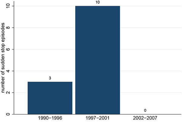
Following Calvo et al. (2004), we define a sudden stop episode as a spell with exceptionally large current account reversals and a recession. We find 13 sudden stop experiences during 1990-2007 across the 23 emerging economies with an outburst of 10 sudden stops between 1997 and 2001.⁴

To highlight the outburst of sudden stops after the mid-1990s, we divide this time frame into three periods as shown in Figure 1: 1990-1996 is a period of low-frequency sudden stops (with 3 occurrences), 1997-2001 is a period of high-frequency sudden stops (with 10 occurrences), and 2002-2007 is a period of low-frequency sudden stops (with no occurrence).

2.2  Foreign Reserves

In the IFS dataset, foreign reserves are defined as all official public sector foreign assets, except gold, that are readily available to and controlled by the monetary authorities. We highlight two notable facts regarding foreign reserves holdings.

Figure 1. Sudden Stops in Emerging Economies

The first fact is that foreign reserves in emerging economies, both as a percent of GDP and and as a percent of external debt liabilities, are significantly higher than those in advanced economies⁵. The second fact is that these ratios have increased in emerging economies while they have decreased in advanced economies. These facts are summarized in Figures 2 and 3.

Figure 2. Foreign Reserves (Percent of GDP)

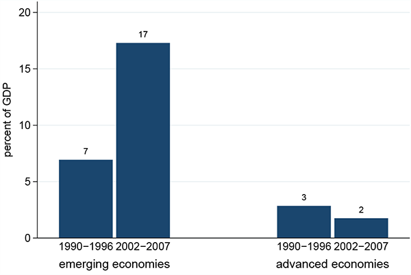
Note: The value for each period and each bloc is the median across economies of the period-average for each economy.

It is worth noting that this phenomenon of increasing reserves is not limited to just a few countries. In fact, foreign reserves are increasing in almost all emerging economies with Chile being the only case in which reserves are decreasing in both measures. This robust observation is shown in Table A.1 (see appendix) of average foreign reserves by country and period.

Figure 3. Foreign Reserves (Percent of External Debt Liabilities)

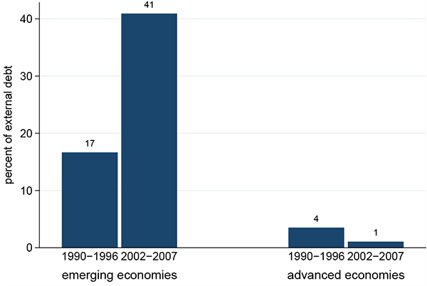
Note: The value for each period and each bloc is the median across economies of the period-average for each economy.

2.3  Reserves and Sudden Stop Probabilities

Following Gourinchas and Obstfeld (2012), we use a panel discrete-choice model to document the effect of foreign reserves on sudden stops. They documented that foreign reserves are associated with reduced banking crisis, currency crisis, or sovereign default. We further document that higher foreign reserves are also associated with reduced sudden stop likelihood. In contrast, net foreign assets are not typically associated with a reduced probability of a crisis.

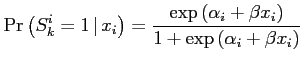
We use a panel logit model with country fixed effects:

$$\Pr\left(S_{k}^{i}=1\,\vert\, x_{i}\right)=\frac{\exp\left(\alpha_{i}+\beta x_{i}\right)}{1+\exp\left(\alpha_{i}+\beta x_{i}\right)}$$

where $S_{k}^{i}$ denotes whether country $i$ is in a sudden stop episode in the next $k$ years and $x_{i}$ are foreign reserves and net foreign assets in country $i$ during a year that is not 0 to 3 years after a sudden stop episode (that is, "tranquil" times using the terminology of Gourinchas and Obstfeld (2012)). The sample is restricted to "tranquil" times to avoid post-crisis bias.

The results of the panel logit estimation are reported in Table 1. Foreign reserves are significantly associated with a reduced probability of sudden stops. For instance, an increase of one standard deviation in the ratio of foreign reserves to external debt liabilities (around 20 percent) is associated with a fall of 7 percent in the probability of a sudden stop over the next two years. The results in Table 1 therefore extend the findings in Gourinchas adn Obstfeld (2012) on the importance of foreign reserves. Table 1 also shows that, unlike foreign reserves, net foreign assets are not commonly associated with crises.⁶ These findings therefore suggest that foreign reserves should be explicitly modeled to understand financial crises in emerging economies. We develop a theory of rollover risk, sudden stops, and foreign reserves in the next section.

3  Model

3.1  Environment

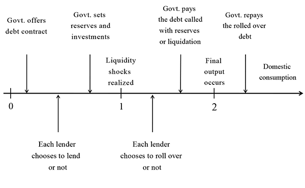
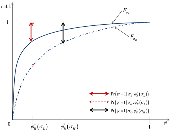
We consider a small open economy model with three stages: s=0 (initial), 1 (interim), 2 (final). There is a unit measure of risk neutral foreign lenders who can lend to the domestic country.⁷ The domestic country has a representative agent who has linear preferences $u(C)=C$ over final stage consumption $C$. The government chooses allocations and debt arrangements to maximize the expected utility of the domestic agent. An overview of the sequence of actions taken by the government and the lenders is presented in Figure 4.

Table 1. Panel Logit Estimation Across Emerging Economies

	S.D.	1-2 Years: δp	1-2 Years: ∂p/∂x	1-3 Years: δp	1-3 Years: ∂p/∂x
Panel A: Sudden Stops: Reserves	20.16	-7.13***	-0.52***	-10.43***	-0.68***
Panel A: Sudden Stops: Reserves over External Debt		(1.45)	(0.14)	(2.28)	(0.19)
Panel A: Sudden Stops: Net Foreign Assets	10.07	-3.86*	0.46	-8.33**	-1.00**
Panel A: Sudden Stops: Net Foreign Assets over GDP		(2.30)	(0.32)	(2.87)	(0.42)
Panel A: Sudden Stops: Probability in percent (p)		11.76		20.37
Panel B: Default Crises: Reserves	21.58	-8.08***	-0.71***	-12.41***	-1.11***
Panel B: Default Crises: Reserves over External Debt		(2.15)	(0.21)	(3.10)	(0.29)
Panel B: Default Crises: Net Foreign Assets	7.79	-3.95*	0.63	-6.16**	-0.98*
Panel B: Default Crises: Net Foreign Assets over GDP		(2.34)	(0.47)	(2.88)	(0.56)
Panel B: Default Crises: Probability in percent (p)		10.11		15.01
Panel C: Banking Crises: Reserves	27.98	-3.92	-0.42**	-7.12**	-0.69***
Panel C: Banking Crises: Reserves over External Debt		(2.47)	(0.17)	(3.00)	(0.18)
Panel C: Banking Crises: Net Foreign Assets	7.42	-0.89	-0.14	-1.64	0.25
Panel C: Banking Crises: Net Foreign Assets over GDP		(0.95)	(0.16)	(1.45)	(0.24)
Panel C: Banking Crises: Probability in percent (p)		4.12		7.67
Panel D: Currency Crises: Reserves	24.54	-2.00	-0.36*	-4.52*	-0.70**
Panel D: Currency Crises: Reserves over External Debt		(1.65)	(0.21)	(2.49)	(0.25)
Panel D: Currency Crises: Net Foreign Assets	8.60	-0.43	0.04	1.95	0.19
Panel D: Currency Crises: Net Foreign Assets over GDP		(0.94)	(0.09)	(2.10)	(0.18)
Panel D: Currency Crises: Probability in percent (p)		2.02		4.62

Note: *, **, and *** denote significance at the 10, 5, and 1 percent level. ∂_p/∂_x is the marginal effect in percentage at "tranquil" sample mean. s.d.(x) is the unconditional standard deviation of x over "tranquil" times. Robust standard errors in parentheses are computed using the delta-method. The estimation sample is an unbalanced panel that spans 20 emerging countries between 1990 and 2007. Currency, banking, and default crises dates follow Gourinchas and Obstfeld (2012).

Figure 4. Timeline

The domestic country has access to two technologies á la Diamond and Dybvig (1983). The first technology transforms the investment $K$ made in the initial stage into $AK$ units in the final stage if production is uninterrupted. However, if production is interrupted in the interim through the liquidation of $L\in[0,K]$ units of investment, the technology yields $\lambda L$ in the interim and $A(K-L)$ in the final stage. We assume that liquidation is costly,

$$\lambda<1.$$ (1)

Further, we impose that there is no partial interim liquidation,

$$L\in\{0,K\}.$$ (2)

This assumption of full liquidation is made for analytical tractability and is relaxed in the next section. The second technology stores resources (reserves) across stages without depreciation. These technologies are summarized by the following table:

Technologies	s=0	s=1	s=2
Production and liquidation	-K investment	λL liquidation	A(K-L) final output
Reserves	-R1 initial reserves	R1
		-R2 interim reserves	R2

In the initial stage, the domestic government borrows $D$ from foreign lenders to finance its initial stage investments,

$$R_{1}+K\leq D.$$ (3)

In the interim, a random fraction $\varphi$ of the foreign lenders receive liquidity shocks denoted by $\varphi^{i}=1$, meaning that they must call the loan and be repaid back. The remaining fraction $\left(1-\varphi\right)$ of lenders with $\varphi^{i}=0$ can call or roll over their loans. The random aggregate liquidity shock $\varphi\in[0,1]$ has a cumulative distribution function that follows the bounded Pareto distribution given by $F_{\sigma}(\varphi)=1-\left(1-\varphi\right)^{1/\sigma}$ with $\sigma>0$.

We denote $\psi^{i}=0$ if lender $i$ rolls over the loan and $\psi^{i}=1$ otherwise. The fraction of lenders calling the loan is: $\psi\equiv\int\psi^{\ell}d\ell$. We assume that individual lenders cannot coordinate on rollover decisions. We call it a sudden stop when all lenders refuse to roll over in the interim ($\psi=1$). However, all lenders may panic and refuse to roll over regardless of the state of the economy. In this paper, we rule out these self-fulfilling "panic" runs, and instead focus on "rational" sudden stops that occur as part of the optimal contract depending on the state of the economy.⁸

We allow the debt repayment of the debt $D$ to be contingent on whether or not the economy is facing a sudden stop. During normal times, foreign lenders receive $P_{1}=D$ if they call the loan in the interim, and $P_{2}=\left(1+r_{N}\right)D$ in the final stage if they roll over the loan.⁹ During a sudden stop, however, all the lenders call the debt and receive $P_{1}=\left(1+r_{S}\right)D$ in the interim. The debt repayment schedule can be summarized as:

	Interim payment P1	Final payment P2
Normal times (ψ<1)	D	(1+rN)D
Sudden stop (ψ=1)	(1+rS)D	0

Because the interest rate can be different when the economy is in sudden stop, the government can choose to partially default during sudden stop episodes by setting $r_{S}<r_{N}$. However, there is a limit to the haircut the lenders can suffer because they can collectively bargain and extract a fraction $\theta$ of the interim resources available $\left(R_{1}+\lambda K\right)$.¹⁰ The constraint arising from this collective bargaining outcome is given by:

$$\left(1+r_{S}\right)D\geq\min\left\{ \left(1+r_{N}\right)D,\theta\left(R_{1}+\lambda K\right)\right\}$$ (4)

In this section, we impose $\theta=1$. This assumption is relaxed in the next section.

3.2  Feasible Debt Contracts

We now define the feasibility constraints that the debt contract offered by the government must satisfy in this environment. First, we define a debt contract as a list of:

• four scalars: $\left\{ R_{1},\,\, K,\,\, r_{N},\,\, r_{S}\right\}$ representing the initial reserves, the invested capital, the normal interest rate, and the sudden stop interest rate, and
• four state-contingent functions: $\left\{ C\left(\varphi\right),\,\, R_{2}\left(\varphi\right),\,\, L\left(\varphi\right),\,\,\psi^{i}\left(\varphi,\varphi^{i}\right)\right\}$ , which denote the final consumption, the interim reserves, the interim liquidation, and the individual rollover policies, respectively.

Resource feasibility  A debt contract is resource feasible if it satisfies equations (2) and (3) as well as the following constraints:

$$R_{2}\left(\varphi\right)+\psi\left(\varphi\right)P_{1}\left(\psi\left(\varphi\right)\right) \leq R_{1}+\lambda L\left(\varphi\right)\quad\forall\varphi$$ (5)

$$C\left(\varphi\right)+\left(1-\psi\left(\varphi\right)\right)P_{2}\left(\psi\left(\varphi\right)\right) \leq R_{2}\left(\varphi\right)+A\left(K-L\left(\varphi\right)\right)\quad\forall\varphi$$ (6)

$$\le R_{1},\; R_{2}\left(\varphi\right),\; C\left(\varphi\right)\quad\forall\varphi.$$ 0 (7)

Equation (5) requires that interim debt payments and interim reserves cannot exceed initial reserves and interim liquidation, while equation (6) requires that final debt payments and consumption cannot exceed interim reserves and final output.

Interim individual rationality  

A debt contract is interim individually rational if, for each aggregate liquidity shock $\varphi$ and individual liquidity shock $\varphi^{i}$,

$V(\psi^{i}\vert\varphi,\varphi^{i})\geq V(1-\psi^{i}\vert\varphi,\varphi^{i})$		(8)
where	$$V(\psi^{i}\vert\varphi,\varphi^{i})=\left\{ \begin{array}[c]{ll} P_{1}(\psi(\varphi)) & \text{if }\psi^{i}=1\ & \ 1_{\varphi_{i=0}}\cdot P_{2}(\psi(\varphi)) & \text{if }\psi^{i}=0 \end{array}\right.$$

This condition requires that the rollover policy yields a payoff at least as high as that from deviating. The lender payoff is given by $P_{1}\left(\psi\left(\varphi\right)\right)$ when calling, and $P_{2}\left(\psi\left(\varphi\right)\right)$ when rolling over, if the lender did not receive a liquidity shock.

Ex ante participation constraint  A debt contract satisfies the ex ante participation constraint if ex ante the debt contract is as profitable as investing at the world interest rate $r_{W}$:

$$\mathbf{E}\left[V\left(\psi^{i}\,\vert\,\varphi,\varphi^{i}\right)\right]\, \geq \,(1+r_{W})D.$$ (9)

Ex post renegotiation proofness  Finally, a debt contract is ex post renegotiation-proof if it satisfies equation (4). This condition limits the haircut suffered by lenders in a sudden stop.

3.3  Optimal Debt Contract

An optimal debt contract is a tuple,

$$B^{*}=\left\{ R_{1}^{*},\, K^{*},\, r_{N}^{*},\, r_{S}^{*},\, C^{*}\left(\varphi\right),\, R_{2}^{*}\left(\varphi\right),\, L^{*}\left(\varphi\right),\,\psi^{i*}\left(\varphi,\varphi^{i}\right)\right\} ,$$

which maximizes the expected utility of the domestic agent subject to resource feasibility, interim individual rationality, the ex ante participation constraint, and ex post renegotiation-proofness. In other words, the government solves:

$\max_{B}E_{\varphi}[C(\varphi)]$
subject to (2)-(9)

3.4  Characterization

We now characterize the solution to the optimal debt contract problem.

Proposition 1. Optimal Debt Contract

An optimal debt contract $B^{*}$ satisfies:

(i) Interim payments are paid exclusively with reserves until they are depleted:

$\exists\quad\varphi_{R}^{*}\in[0,1]\;$s.t.$\;\begin{cases} R_{2}^{*}(\varphi)>0 & \iff\varphi\in[0,\varphi_{R}^{*})\ L^{*}(\varphi)=0 & \iff\varphi\in[0,\varphi_{R}^{*}) \end{cases}$

Furthermore, the optimal reserves ratio is: $\varphi_{R}^{*}=\dfrac{R_{1}^{*}}{D}=1-\left[\dfrac{A-1}{A-\lambda}\left(\dfrac{\sigma}{\sigma+1}\right)\right]^{\sigma}$ .

(ii) For sufficiently large aggregate shocks, all lenders call their loans:

$\exists\quad\varphi_{S}^{*}\in[0,1]\;$s.t.$\;\begin{cases} \psi(\varphi)=\varphi & \forall\varphi\in[0,\varphi_{S})\ \psi(\varphi)=1 & \forall\varphi\in[\varphi_{S},1] \end{cases}$

Furthermore, sudden stops occur whenever reserves are depleted: $\varphi_{S}^{*}=\varphi_{R}^{*}$.

Proof: See appendix.

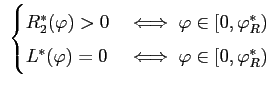
Proposition 1(i) and 1(ii) establish that there are cutoff rules for reserves, liquidation, and sudden stops. In Proposition 1(i), $\varphi_{R}^{*}$ is the liquidity shock at which reserves are depleted and the government must liquidate the invested capital to meet the promised payments. Because $\lambda<1$, the government uses existing reserves to meet payments before eventually liquidating the invested capital. Proposition 1(i) also establishes that the optimal reserves-to-liabilities ratio is $\varphi_{R}^{*}$.

In Proposition 1(ii), $\varphi_{S}^{*}$ is the liquidity shock above which all lenders exit. We identify this debt rollover crisis as a sudden stop. The sudden stop cutoff $\varphi_{S}^{*}$ is equal to the optimal reserves-to-debt ratio $\varphi_{R}^{*}$ because we assumed there is no partial liquidation. A sudden stop therefore occurs as soon as the normal interim payments cannot be met using reserves. We later relax the full liquidation assumption. With partial liquidation, the sudden stop cutoff and the reserves cutoff no longer coincide.

The following corollary establishes the endogenous relation between the optimal reserves and the probability of sudden stops. In this environment, reserves are set to balance the sudden stop risks incurred when reserves are not high enough and the cost of holding idle reserves.

Corollary 1. Endogenous Sudden Stop Probability

The optimal contract $B^{*}$ induces a positive probability $\Pr\left(\psi=1\right)>0$ that a sudden stop occurs. Furthermore, $\Pr\left(\psi=1\right)=1-F_{\sigma}\left(\varphi_{R}^{*}\right)$ .

Proof: This follows immediately from Proposition 1.

3.5  Comparative Statics

In this subsection, we discuss how reserves and sudden stop probabilities are affected by changes in the underlying liquidity risk, that is: changes in $\sigma$.

Proposition 2. Reserves, Sudden Stop Probability, and Debt Rollover Risk

(i) The optimal reserves ratio is increasing in the aggregate liquidity risk. That is:

$$\dfrac{\partial\varphi_{R}^{*}}{\partial\sigma}>0$$

(ii) The sudden stop probability is also increasing in the aggregate liquidity risk. That is:

$$\dfrac{\partial\Pr\left(\psi\left(\varphi\right)=1\;\vert\;\sigma\right)}{\partial\sigma}>0$$

Proof: See appendix.

Proposition 2 establishes that both the optimal reserves and the implied sudden stop probability are increasing in the liquidity risk. A larger liquidity risk $\sigma$ induces larger interim shocks and prompts the domestic government to invest in additional reserves. However, the increase in reserves does not completely offset the higher probability of larger shocks, thus leading to an increase in the debt rollover risk. Based on this proposition, we simply refer to the aggregate liquidity risk parameter $\sigma$ as "rollover risk" throughout the paper.

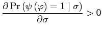
Figure 5. Sudden Stop and Debt Rollover Risk

A central question that we address using Proposition 2 is: what happens during an unexpected increase in rollover risk, say in the wake of globalization? Figure 5 shows how an unexpected increase in $\sigma$ from $\sigma_{L}$ to $\sigma_{H}>\sigma_{L}$ leads to a increase in sudden stop probability as represented by the dashed vertical line. Obviously, the government does not hold enough reserves, given the unexpected increase in rollover risk. We later show quantitatively that a small, but unanticipated increase in rollover risk leads to a short-lived outburst of sudden stops and a dramatic rise in reserves as seen in the data.

3.6  Self-Insurance Versus Mutual Insurance

In the self-insurance setup above, a government faces aggregate uncertainty stemming from its debt rollover risk. An individual government may over-accumulate reserves compared to a world in which governments can pool reserves and mutually insure against their idiosyncratic rollover risk. We now characterize the extent of reserves over-accumulation.

For simplicity, consider the problem of a planner who can swap resources across a continuum of countries facing i.i.d. idiosyncratic liquidity shocks $\varphi^{j}$ with c.d.f. $F_{\sigma}$. By the law of large numbers, the total measure of lenders who must call the debt is $\mathbf{E}\left[\varphi\right]=\sigma/\left(\sigma+1\right)$. In that sense, there is no aggregate uncertainty across countries as they insure each other.¹¹

In fact, the planner could set reserves to $\mathbf{E}\left[\varphi\right]$ and thereby prevent any sudden stop from occurring in any country. This policy is indeed optimal when the liquidity risk is sufficiently low.

Proposition 3. Self-Insurance Versus Mutual Insurance

Consider a continuum of countries subject to i.i.d. liquidity shocks. Each country individually over-accumulates reserves compared to the mutual insurance outcome $\varphi_{R}^{C}$. That is:

$$\varphi_{R}^{*}>\mathbf{E}\left[\varphi\right]\ge\varphi_{R}^{C}\qquad\forall\sigma\in\left(0,1\right)$$

Moreover, if $\sigma\le\left(1-\lambda\right)/A$, then $\mathbf{\varphi_{R}^{C}=E}\left[\varphi\right]$.

Proof: See appendix.

Proposition 3 establishes that countries hold more reserves than needed if they could mutually insure against idiosyncratic liquidity shocks. The mutual insurance problem has similarities with the liquidity provision problem studied by Holmström and Tirole (1998). Under mutual insurance, economies that face large liquidity shocks in the interim can access the reserves of economies with small liquidity needs, thereby reducing the overall debt rollover risk and the reserves required to manage it. In the next section, we quantify the over-accumulation of reserves after calibrating the liquidity risk faced by emerging economies.

4  A Multi-Country Dynamic Application

The previous section highlighted the relationship between rollover risk, sudden stops, and reserves. In this section, we extend this model along two dimensions.

First, the model is extended to an infinite horizon environment in which each period $t$ contains the three stages, $s=0,1,2$, of the basic model. At the end of each period $t$, the government chooses how much reserves to transfer to the next period. Second, the model is extended to a multi-country environment in which agents learn about the underlying rollover risk, $\sigma_{t}$, using information on the sudden stop occurrences each period.

4.1  Environment

We consider $N$ identical small economies indexed by $j=1,\ldots,N$. Time is infinite, discrete, and indexed by $t=0,1,\ldots,\infty$. Each country is populated by an infinitely-lived representative agent and a welfare-maximizing government. The agents in country $j$ order consumption sequences according to $\mathbf{E}_{0}\left[\sum_{t=0}^{\infty}\beta^{t}C_{t}^{j}\right]$ where $\beta$ is the discount factor. There is a continuum of infinitely lived risk-neutral foreign lenders indexed by $i\in\left[0,1\right]$. An overview of the timeline of this extended model is showed in Figure 6.

Figure 6. Extended Timeline

Each time period $t$ is divided into three stages, $s=0,1,2$, and encapsulates the three stages of the previous model:

• $s=0$ is the initial contracting stage,
• $s=1$ is the interim stage when liquidity shocks occur and rollovers decided,
• $s=2$ is the final production and consumption stage.

The aggregate interim liquidity shock in country $j$ at time $t$ is denoted by $\varphi_{t}^{j}\in\left[0,1\right]$. As in the basic model, this means that a fraction $\varphi_{t}^{j}$ of country $j$'s creditors must call the debt in the interim while the others can roll over or call the debt. The aggregate shocks $\left\{ \varphi_{t}^{j}\;:\; j=1\ldots\, N\right\} _{t=0}^{\infty}$ are independent and identically distributed across countries and time, with cumulative distribution function $F_{\sigma_{t}}\left(\varphi\right)=1-\left(1-\varphi\right)^{1/\sigma_{t}}$ . We assume $\sigma_{t}\in\left\{ \sigma_{L},\sigma_{H}\right\}$ with $\sigma_{L}<\sigma_{H}$.

This rollover risk parameter $\sigma_{t}$ is unobserved and unknown to the agents. However, all agents share a common belief $\rho_{t}$ at time $t$:

$$\rho_{t}\equiv\Pr\left(\sigma_{t}=\sigma_{L}\right)$$

At the end of each period $t$, agents observe the sudden stop occurrences in the $N$ countries. Using these sudden stop occurrences and the endogenous sudden stop probabilities, agents update their beliefs according to Bayes' rule as detailed in section 4.3.

Within each period $t$, the technologies available at a stage $s$ are identical to those in the previous section.¹² In addition, at the end of each period, the government can save $R_{0,t+1}^{j}$ reserves for the next period using the remaining reserves $R_{2,t}^{j}$:

$$R_{0,t+1}^{j}\in\left[0\;,\; R_{2,t}^{j}\right].$$

We now allow for partial liquidation in the interim:

$$L_{t}^{j}\in\left[0,\; K_{t}^{j}\right].$$

This implies that sudden stops may not occur as soon as reserves are depleted.

4.2  Optimal Recursive Debt Contracts

We represent the government's infinite horizon problem as a recursive dynamic programming problem. The problem has one endogenous state, the level of incoming saved reserves, $R_{0,t}^{j}$, and one exogenous state, the common belief, $\rho_{t}$. The state of economy $j$ at time $t$ is then given by $\left(R_{0};\rho\right)=\left(R_{0,t}^{j};\rho_{t}\right)$.

The optimal recursive debt contract, $B^{*}\left(R_{0};\rho\right)$, is a set of policy functions for initial reserves: $R_{1}\left(R_{0};\rho\right)$, invested capital: $K\left(R_{0};\rho\right)$, normal interest rates: $r_{N}\left(R_{0};\rho\right)$, sudden stop interest rates: $r_{S}\left(R_{0};\rho\right)$, sudden stop cutoffs: $\varphi_{S}\left(R_{0};\rho\right)$, consumption: $C\left(R_{0},\varphi;\rho\right)$, interim reserves: $R_{2}\left(R_{0},\varphi;\rho\right)$, liquidation: $L\left(R_{0},\varphi;\rho\right)$, saved reserves: $R_{0}'\left(R_{0},\varphi;\rho\right)$, and rollover policies: $\psi^{i}\left(R_{0},\varphi,\varphi^{i};\rho\right)$ which satisfy the functional equation:

$$\begin{array}{ccc} W\left(R_{0};\rho\right)= & \underset{B\in\Gamma\left(R_{0}\right)}{\max} & \mathbf{E}{}_{\varphi\vert\,\rho}\,\left[u\left(C\left(\varphi\right)\right)+\beta W\left(R_{0}';\rho\right)\right]\end{array}$$

As in the previous section a debt contract is feasible, that is, $B\in\Gamma\left(R_{0}\right)$, if it satisfies resource feasibility, interim individual rationality, the ex ante participation constraint, and ex post renegotiation proofness. Resource feasibility is modified to allow for saved reserves and partial liquidation. The initial $(s=0)$ resource constraint, which incorporates incoming reserves saved ($R_{0}$), is now:

$$R_{1}+K\leq D{\color{red}\,\,+\,\, R_{0}.}$$ (10)

The final $(s=2)$ resource constraint, modified to allow for inter-temporal reserves savings ( $R_{0}^{'}\left(\varphi\right)$), is now:

$$C\left(\varphi\right)+\left(1-\psi\left(\varphi\right)\right)P_{2}\left(\psi\left(\varphi\right)\right)\leq R_{2}\left(\varphi\right){\color{red}-\,\, R_{0}'\left(\varphi\right)}+A\left(K-L\left(\varphi\right)\right).$$ (11)

Also, saved reserves and liquidation must satisfy

$$R_{0}'\left(\varphi\right) \in \left[0\;,\; R_{2}\left(\varphi\right)\right]\quad\forall\varphi$$ (12)

$$L\left(\varphi\right) \in \left[0\;,\; K\right]\quad\forall\varphi$$ (13)

4.3  Bayesian Learning

The common belief $\rho_{t}\equiv\Pr\left(\sigma_{t}=\sigma_{L}\right)$ is dynamically updated using the sudden stop occurrences and sudden stop probabilities in the $N$ countries.¹³ Let us denote $\chi_{t}\in\left\{ 0,1\right\} ^{N}$ as the vector of sudden stops where $\chi_{t}^{j}=1$ denotes that country $j$ experienced a sudden stop in period $t$. For each country $j$, given the incoming reserves $R_{0,t}^{j}$, the probability of a sudden stop $\Pr\left(\chi_{t}^{j}\vert R_{0,t}^{j};\rho_{t}\right)$ is endogenously determined by the optimal policy for the prevailing belief $\rho_{t}$.

Bayes' Rule implies that:

$${\displaystyle \rho_{t+1}={\displaystyle \frac{\rho_{t}\Pr\left(\chi_{t}\;\vert\;\sigma_{L}\right)}{\rho_{t}\Pr\left(\chi_{t}\;\vert\;\sigma_{L}\right)+(1-\rho_{t})\Pr\left(\chi_{t}\;\vert\;\sigma_{H}\right)}}}$$

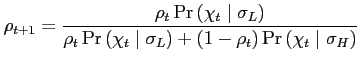
with the joint endogenous sudden stop probabilities $\Pr\left(\chi_{t}\;\vert\;\sigma_{t}\right)$ given by:

$${\displaystyle \begin{array}{rl} \Pr\left(\chi_{t}\vert\sigma_{L}\right) & \equiv{\displaystyle \prod_{j=1}^{N}}\Pr\left(\chi_{t}^{j}\vert R_{0,t}^{j};\rho_{t}=1\right)\ \text{and}\ \Pr\left(\chi_{t}\vert\sigma_{H}\right) & \equiv{\displaystyle \prod_{j=1}^{N}}\Pr\left(\chi_{t}^{j}\vert R_{0,t}^{j};\rho_{t}=0\right) \end{array}}$$

where $\Pr\left(\chi_{t}^{j}=1\vert R_{0,t}^{j};\rho_{t}=1\right)=1-F_{\sigma_{L}}\left(\varphi_{S}\left(R_{0,t}^{j};\rho_{t}=1\right)\right)$

and $\Pr\left(\chi_{t}^{j}=1\vert R_{0,t}^{j};\rho_{t}=0\right)=1-F_{\sigma_{H}}\left(\varphi_{S}\left(R_{0,t}^{j};\rho_{t}=0\right)\right)$ .

4.4  Quantitative Analysis

In this section, we use the calibrated model to establish how a small but unexpected increase in debt rollover risk can explain the sharp increase in reserves and the temporary outburst in sudden stops documented in section 2. Based on our theory, an unexpected increase in the rollover risk will temporarily cause an underinvestment in reserve holdings which increases the probability of sudden stops. Governments and investors, seeing the rise in sudden stops, rationally update their common belief about the prevailing debt rollover risk. Once agents have fully learned the new regime, reserves remain steadily higher and sudden stops subside.

Calibration  A period in the model is assumed to be a quarter. We choose $N=23$ as we have 23 emerging economies in our dataset. We assume the aggregate liquidity shock distributions $\left(F_{\sigma_{L}},F_{\sigma_{H}}\right)$ belong to the class of Pareto distributions on $\left[0,1\right]$: $F_{\sigma}\left(\varphi\right)\equiv1-\left(1-\varphi\right)^{1/\sigma}$ . An increase in $\sigma$ shifts the cumulative distribution function $F_{\sigma}$ to the right as illustrated in Figure 5. An increase from $\sigma_{L}$ to $\sigma_{H}$ therefore represents an increase in the underlying debt rollover risk.

The discount factor $\beta$ is set to match average interest rates of two percent in emerging economies over 1990-2007 and the world interest rate $r_{W}$ is set to match a risk-free rate of one percent. The bargaining parameter $\theta$ is set to match the average haircut of 19.4 percent in sovereign defaults from 1990 to 2007 using the data from Benjamin and Wright (2009). The debt rollover risk parameter $\sigma_{L}$ and $\sigma_{H}$ are set to match median reserves-to-debt ratios in the emerging economies for the periods of 1990-1996 and 2002-2007 respectively. We set the liquidation cost $1-\lambda$ to be 25 percent, which is conservative relative to the range of estimates and values used in the literature.¹⁴ The long-term technology productivity $A$ is set to 1.2.¹⁵ The parameters are summarized in Table 2. See the computation appendix in section 6.2 for details on the computation and calibration strategy.

Table 2. Calibration Values

Name	Symbol	Value	Target
Discount factor	β	0.98	average interest rates (emerging)
World interest rate	rW	0.01	risk-free rate
Low rollover risk	σL	0.061	average reserves-to-debt, 1990-1996
High rollover risk	σH	0.172	average reserves-to-debt, 2002-2007
Divestment parameter	λ	0.75	see discussion
Productivity	A	1.2	-
Bargaining parameter	θ	0.965	average haircut on sovereign debt
Number of economies	N	23	emerging countries in sample

Quantitative Results  We assume that after 1996, there was an unexpected increase from a $\sigma_{L}$-regime to a $\sigma_{H}$-regime. This is motivated by the idea that globalization and widespread financial liberalization led to an unprecedented increase in capital mobility and debt rollover risk.

The $N$ ex ante identical economies experience different aggregate liquidity shock paths $\left\{ \varphi_{t}^{j}\right\} _{j,t}$. As a result, their reserves holdings and sudden stops paths also evolve differently. The results shown are the average across a large number of simulated paths for these $N$ countries.

Table 3 summarizes our key results. The calibration reveals that the debt rollover risk $\sigma$ increased from 0.061 to 0.172. This is a small increase in the sense that the implied sudden stop probabilities only rise from 0.06 percent to 0.19 percent, compared to a 1.58 percent probability during the transition. Despite this small increase in debt rollover risk, there is an outburst of sudden stops with the mode across simulations reaching 7 before subsiding (see Figure 7). In the meantime, the optimal reserves-to-debt ratios climbed from 17 percent to 41 percent. The temporary surge in sudden stops is consistent with our discussion of Proposition 2 in the simple model (see Figure 5): as governments learn the higher rollover risk, they choose to hold a higher level of reserves, thus returning sudden stop probabilities to lower levels. The calibration establishes quantitatively how a small increase in rollover risk can explain the surge we observed in the data. As can be seen in Figure 8, our model can jointly generate the temporary outburst of sudden stops in the transition (1997-2001) along with the permanent rise in reserves ever since.

Table 3. Summary of Results

	1990-1996	1997-2001	2002-2007
Data: Reserves-to-External Debt Liabilities	0.17	0.28	0.41
Data: Sudden Stops	2	10	0
Model: Reserves-to External Debt Liabilities	0.17	0.33	0.41
Model: Sudden Stops	0.40	7.28	1.10
Model: Rollover Risk (σ)	0.061	0.172	0.172
Model: Sudden Stop Probabilities (percent)	0.06	1.58	0.19

International Mutual Insurance and Reserves  Proposition 3 showed that countries over-accumulate reserves compared to an allocation with mutual insurance with other countries. We now use the calibrated parameters to quantify the magnitude of the over-accumulation of reserves due to self-insurance.

Given the calibrated parameter values and using Proposition 3, the international planner facing no aggregate uncertainty will optimally set reserves to the mean liquidity shock because $\sigma_{H}<(1-\lambda)/A$. Therefore, in the higher rollover risk $\left(\sigma_{H}\right)$ regime, the international planner optimally sets the reserves-to-debt ratio at: $\sigma_{H}/\left(1+\sigma_{H}\right)=14.68$ percent. This amounts to nearly one-thirds of the level of 41 percent in reserves-to-debt that emerging economies held from 2002 to 2007.¹⁶

This result clearly underscores the importance of mutual insurance or international coordination across governments facing uninsurable idiosyncratic debt rollover risk. In fact, during the recent global financial crisis, reserves swap agreements such as the ASEAN+3 Chiang Mai Initiative were expanded. The U.S. and Japan also extended swap lines to emerging economies such as Korea.

The IMF could in principle assume the role of an international planner for rollover risk insurance. However, many economists and policymakers argue (see Ito (2012)) that emerging economies still bear the scar and the stigma from the inadequate liquidity assistance provided by the IMF during the crises of the late 1990s.

Figure 7. Histogram of Sudden Stops Frequencies by Era

Figure 8. Results - Reserves and Sudden Stops

Reserves in the Euro Area Periphery Economies  Interestingly, before 1999, the Euro Area Periphery economies (Greece, Ireland, Italy, Portugal, Spain) held the same levels of reserves as the 23 emerging economies we consider. However, upon joining the Euro Area, these economies slashed their reserves holdings, as illustrated in Figure 9.¹⁷

The common currency certainly explains part of the reduction in foreign reserves. However, to the extent that these economies still faced debt rollover risk, they may have under-invested in reserves. For instance, they may have mistakenly believed that they no longer faced rollover risk as they joined the Euro. Alternatively, the Periphery economies ex ante may have counted on a mutual insurance policy against liquidity needs which showed its limits during the Euro crisis.

In the meantime, self-insurance through reserves helped emerging economies weather the global financial crisis as noted by Dominguez et al. (2012) as well as Gourinchas and Obstfeld (2012). This is also consistent with our findings on the preventive role of reserves.

Figure 9. Foreign Reserves in the Euro Area Periphery

Note: The value for each period and each bloc is the median across economies of the period-average for each economy.

5  Conclusion

In this paper, we developed a theory of rollover risk, sudden stops, and reserves that can jointly account for the dynamics of foreign reserves and sudden stops in emerging economies.

In our theory, governments choose reserves to prevent "patient" foreign creditors from refusing to rollover their claims and inducing a sudden stop. We calibrate a dynamic multi-country extension of the model with Bayesian learning to emerging economies. A small, unexpected, but permanent change in rollover risk leads to the surge in sudden stops in the late 1990s, the subsequent rise in reserves, and the salient fall in sudden stops ever since. We also find that a policy of international mutual insurance can substantially reduce the reserves held by emerging economies.

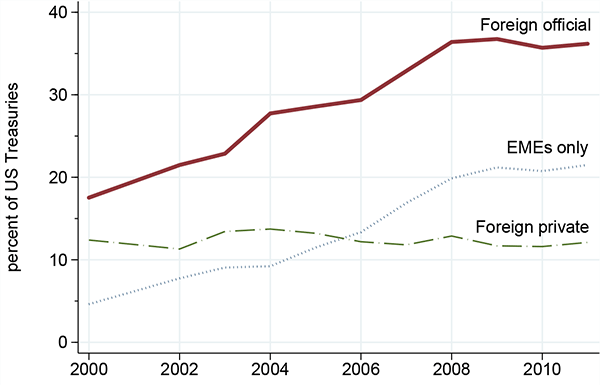
Several caveats are in order. Our model ignores the decision to issue reserve assets. In particular, U.S. Treasuries, the most popular reserve asset, are being increasingly held by foreign officials as they accumulate reserves (see Figure 10). Can the U.S. sustainably issue large amounts of reserve assets? Moreover, our model does not consider the maturity composition of a country's debt. We leave these interesting considerations for future research.

Figure 10: Foreign Holdings of U.S. Treasuries

Bibliography

Aizenman, Joshua, and Lee, Jaewoo. 2007. "International Reserves: Precautionary versus Mercantilist views, Theory and Evidence." Open Economies Review, 18(2): 191-214.

Alderson, Michael J., and Brian L. Betker. 1996. "Liquidation costs and accounting data." Financial Management, 25(2): 25-36.

Alfaro, Laura and Kanczuk, Fabio. 2009. "Optimal Reserve Management and Sovereign Debt." Journal of International Economics, 77(1):23-36.

Akinci, Ozge. 2012. "Global Financial Conditions, Country Spreads and Macroeconomic Fluctuations in Emerging Countries: A Panel VAR Approach."Working Paper.

Arellano, Cristina, and Ananth Ramanarayanan. 2012. "Default and the Maturity Structure in Sovereign Bonds." Journal of Political Economy, 120(2): 187-232.

Benjamin, David, and Mark L. J. Wright. 2009. "Recovery Before Redemption: A Theory of Delays in Sovereign Debt Renegotiations." Working Paper.

Bernanke, Ben. 2005. "The Global Saving Glut and the U.S. Current Account Deficit." Remarks at the Sandridge Lecture, Virginia Association of Economists, Richmond, Virginia, March 10, 2005.

Brown, Richard A., and Seth Epstein. 1992. "Resolution costs of bank failures: An update of the FDIC historical loss model." FDIC Banking Review, 5(2): 1-16.

Bianchi, Javier, Juan Carlos Hatchondo, and Leonardo Martinez. 2012. "International Reserves and Rollover Risk." Working paper.

Broner, Fernando A., Guido Lorenzoni, and Sergio L. Schmukler. 2007. "Why do Emerging Economies Borrow Short Term?" NBER Working Paper No. w13076.

Buera, Francisco J., Alexander Monge-Naranjo, and Giorgio E. Primiceri. 2011. "Learning the Wealth of Nations." Econometrica, 79(1): 1-45.

Caballero, Ricardo, and Stavros Panageas. 2007. "A Quantitative Model of Sudden Stops and External Liquidity Management." NBER Working Paper No. w11293.

Calvo, Guillermo A., Alejandro Izquierdo, and Rudy Loo-Kung. 2012. "Optimal Holdings of International Reserves: Self-Insurance Against Sudden Stops." NBER Working Paper No. w18219.

Calvo, Guillermo A., Alejandro Izquierdo, and Luis-Fernando Mejia. 2004. "On the Empirics of Sudden Stops: The Relevance of Balance-Sheet Effects." NBER Working Paper No. 10520.

Chang, Roberto, and Andres Velasco. 2001. "A model of financial crises in emerging markets." The Quarterly Journal of Economics, 116(2): 489-517.

Cole, Hal L. and Timothy J. Kehoe. 2000. "Self-Fulfilling Debt Crises." Review of Economic Studies, 67(1): 91–116.

Diamond, Douglas W., and Philip H. Dybvig. 1983. "Bank Runs, Deposit Insurance, and Liquidity." Journal of Political Economy, 91(3): 401–419.

Dominguez, Kathryn ME, Yuko Hashimoto, and Takatoshi Ito. 2012. "International reserves and the global financial crisis." Journal of International Economics, 88(2): 388-406.

Dooley, Michael P., David Folkerts-Landau, and Peter Garber. 2004. "The Revived Bretton Woods System." International Journal of Finance and Economics, 9(4): 307-313.

Durdu, Ceyhun Bora, Enrique G. Mendoza, and Marco E. Terrones. 2009. "Precautionary Demand for Foreign Assets in Sudden Stop Economies: An Assessment of the New Mercantilism." Journal of Development Economics, 89(2): 194-209.

Ennis, Huberto M., and Todd Keister. 2003. "Economic Growth, Liquidity, and Bank Runs." Journal of Economic Theory, 109(2): 220–245.

Frenkel, Jacob, and Boyan Jovanovic. 1981. "Optimal International Reserves: A Stochastic Framework." The Economic Journal, 91(362): 507-514.

Gendreau, Brian C., and Scott S. Prince. 1986. "The Private Costs of Bank Failures: Some Historical Evidence." Federal Reserve Bank of Philadelphia Business Review, March/April: 3-14.

Gourinchas, Pierre-Olivier and Maurice Obstfeld. 2012. "Stories of the Twentieth Century for the Twenty-First." American Economic Journal: Macroeconomics, 4(1): 226–65.

Heller, Heinz Robert. 1966. "Optimal International Reserves." The Economic Journal, 76(302): 296-311.

Holmström, Bengt, and Jean Tirole. 1998. "Private and Public Supply of Liquidity."The Journal of Political Economy, 106(1): 1-40.

International Monetary Fund. 2012. "Assessing the Need for Foreign Currency Reserves."IMF Survey Magazine: Policy.

Ito, Takatoshi. 2012. "Can Asia Overcome the IMF Stigma?" American Economic Review, 102(3): 198-202.

James, Christopher. 2012. "The losses realized in bank failures." The Journal of Finance, 46(4):1223-1242.

Jeanne, Olivier and Romain Ranciere. 2011. "The Optimal Level of International Reserves for Emerging Market Countries: A New Formula and Some Applications."The Economic Journal, 121: 905–930.

Kehoe, Timothy J., Kim J. Ruhl, and Joe Steinberg. 2012. "A Sudden Stop to the Savings Glut and the Future of the U.S. Economy," Federal Reserve Bank of Minneapolis Research Department Staff Report.

Kim, Jun Il. 2008. "Sudden Stops and Optimal Self-Insurance." IMF Working Papers, No 8144.

Lane, Philip R., and Gian Maria Milesi-Ferretti (2007). "The External Wealth of Nations Mark II: Revised and Extended Estimates of Foreign Assets and Liabilities, 1970–2004." Journal of International Economics, 73(4): 223–25.

Mendoza, Enrique G. 2010. "Sudden stops, financial crises, and leverage." American Economic Review, 100(5): 1941-1966.

Morris, Stephen, and Hyun Song Shin. 1998. "Unique equilibrium in a model of self-fulfilling currency attacks." American Economic Review, 88(3): 587-597.

Morris, Stephen, and Hyun Song Shin. 2006. "Catalytic finance: When does it work?" Journal of international Economics, 70(1): 161-177.

Obstfeld, Maurice, Jay C. Shambaugh, and Alan M. Taylor. 2010. "Financial Stability, the Trilemma, and International Reserves." American Economic Journal: Macroeconomics, 2(2): 57-94.

Yue, Vivian. 2010. "Sovereign Default and Debt Renegotiation." Journal of International Economics, 80(2): 176-187.

6  Appendix

6.1  Tables

Table A.1. Foreign Reserves

	(percent of GDP) 1990-1996	(percent of GDP) 2002-2007	(percent of External Debt Liabilities) 1990-1996	(percent of External Debt Liabilities) 2002-2007
Argentina	4.9	13.5	14.3	21.4
Brazil	4.9	8.6	19.5	35.3
Chile	20.4	16.5	50.9	39.0
China	8.4	33.2	54.3	271.4
Colombia	9.9	10.8	35.6	35.1
Czech Republic	17.4	25.3	57.2	77.5
Egypt	20.9	19.8	35.2	65.5
Hungary	15.5	16.6	26.6	26.2
India	3.5	18.4	11.8	101.0
Indonesia	6.5	12.4	11.7	25.2
Korea	5.4	24.6	28.0	97.4
Malaysia	28.5	47.1	77.0	125.6
Mexioc	4.6	8.2	12.2	40.9
Morocco	10.4	28.6	15.9	99.1
Pakistan	1.8	10.4	4.3	28.2
Peru	11.2	18.4	16.7	49.1
Philippines	8.0	17.3	13.3	28.4
Poland	6.9	14.2	15.9	35.8
Romania	4.2	18.5	22.7	53.9
Russia	3.0	23.2	7.3	68.5
South Africa	1.0	7.1	4.7	34.9
Thailand	19.3	30.6	41.8	112.1
Turkey	3.9	10.9	13.0	25.5

Table A.2. Sensitivity Analysis

	1990-1996	1997-2001	2002-2007
λ = 0.7: Reserves-to External Debt Liabilities	0.17	0.32	0.41
λ = 0.7: Sudden Stops	0.40	7.56	1.22
λ = 0.7: Rollover Risk (σ)	0.058	0.161	0.161
λ = 0.7: Suddent Stop Probabilities (percent)	0.06	1.64	0.21
λ = 0.8: Reserves-to External Debt Liabilities	0.17	0.33	0.41
λ = 0.8: Sudden Stops	0.26	7.60	1.69
λ = 0.8: Rollover Risk (σ)	0.061	0.198	0.198
λ = 0.8: Suddent Stop Probabilities (percent)	0.04	1.65	0.19

Computational Appendix

The computation strategy involves solving for policy functions and simulating the induced equilibrium paths with Bayesian learning. The government problem has two state variables: (i) the incoming reserves, $R_{0}$, and (ii) the belief, $\rho$. The policy functions are : (i) the initial reserves, $R_{1}$, (ii) the sudden stop policy, $\varphi_{S}$,¹⁸ (iii) the liquidation policy, $L(\varphi)$, and (iv) the saved reserves, $R_{0}'(\varphi)$, where $\varphi$ is the interim aggregate liquidity shock. These policy functions are solved by value function iteration. We discretize the state space and decision variables by choosing a finite grid, and use interpolation methods.

Algorithm for Solving Equilibrium and Calibration

1. Guess a vector of parameters $\left\{ \sigma_{L},\sigma_{H},\theta\right\}$
2. For each belief on the belief grid, using value function iteration, solve for value functions and policy functions.
3. Set initial reserves for $N$ countries $\left\{ R_{0,0}^{j}\right\} _{j=1,..,N}=\mathbf{0}$, and initial belief $\rho_{0}=0.97$
4. For $t=1,...,T$,
   1. Set $$\sigma_{t}=\left\{ \begin{array}[c]{lll} \sigma_{L} & & \text{if }t<T_{1}\ & & \ \sigma_{H} & & \text{if }t\geq T_{1} \end{array}\right.$$
   2. Draw aggregate liquidity shocks $\left\{ \varphi_{t}^{j}\right\} _{j=1,..,N}$ from $F_{\sigma_{t}}$
   3. Using distribution of incoming reserves, $\left\{ R_{0,t}^{j}\right\} _{j=1,..,N}$, policy functions, $R_{1}\left(R_{0,t}^{j};\rho_{t-1}\right),\varphi_{S}\left(R_{0,t}^{j};\rho_{t-1}\right),L\left(R_{0,t}^{j},\varphi_{t}^{j};\rho_{t-1}\right),$

      $R_{0}'\left(R_{0,t}^{j},\varphi_{t}^{j};\rho_{t-1}\right)$, and shock realizations, $\left\{ \varphi_{t}^{j}\right\} _{j=1,..,N}$, compute distribution of saved reserves, $\left\{ R_{0,t+1}^{j}\right\} _{j=1,..,N}$

   4. using sudden stop probabilities and realizations, compute posterior as detailed in section 4.3
5. Repeat step 4$M$ times, compute averages over $M$ simulations. When computing averages, exclude $t=1,..,5$.
6. Repeat steps 1-5 until the difference between model moments and corresponding data targets are less than a specified threshold.

6.3  Proofs

PROOF OF PROPOSITION 1:

We proceed in eight steps.

Step 1: Interest rates satisfy

$$r_{S}^{*}<0<r_{N}^{*}$$ (14)

$1+r_{N}^{*}\ge1$ follows from equation (8). Equation (3) and $\lambda<1$ imply that $R_{1}+\lambda K<D$. Since $\theta=1$, equation (4) implies $1+r_{S}^{*}=\left(R_{1}+\lambda K\right)/D$. Hence $r_{S}^{*}<r_{N}^{*}$.

Step 2: If $\psi^{*}(\varphi)=1$, then

$$L^{*}(\varphi) = K^{*}$$ (15)

$$R_{2}^{*}(\varphi) = 0$$ (16)

$$C^{*}(\varphi) = 0$$ (17)

By definition, if $\psi^{*}(\varphi)=1$, then $P_{1}^{*}(\varphi)=\left(1+r_{S}^{*}\right)D$. From step 1, we have that $r_{S}^{*}=\left(R_{1}+\lambda K\right)/D$. Equations (5) and (7) imply equations (15) and (16). Then equation (17) follows from equations (6) and (7) .

Step 3: If $\psi^{*}(\varphi)=\varphi$, then

$$L^{*}(\varphi) = 0$$ (18)

$$R_{2}^{*}(\varphi) = R_{1}^{*}-\varphi D$$ (19)

$$C^{*}(\varphi) = AK^{*}+R_{2}^{*}(\varphi)-\left(1-\varphi\right)\left(1+r_{N}^{*}\right)D$$ (20)

By definition, if $\psi^{*}(\varphi)=\varphi$, then $P_{1}^{*}(\varphi)=D$ and $P_{2}^{*}(\varphi)=\left(1+r_{N}^{*}\right)D$. Suppose for contradiction that $L^{*}(\varphi)=K$. Then equation (5) implies $R_{2}^{*}(\varphi)=R_{1}^{*}+\lambda K^{*}-\varphi D$. Then we have that

$$\begin{eqnarray*} C^{*}(\varphi) & = & R_{1}^{*}+\lambda K^{*}-\varphi D-\left(1-\varphi\right)\left(1+r_{N}^{*}\right)D\ & \le & R_{1}^{*}+\lambda K^{*}-D\ & < & 0 \end{eqnarray*}$$

where the first equality comes from equation (6), the second inequality comes from $1+r_{N}^{*}\ge1$, and the third inequality comes from (3) and $\lambda<1$. This violates equation (7). Hence equation (18) holds. Then equation (19) follows from equation (5), and equation (20) follows from (6).

Step 4: If $\psi^{*}(\varphi_{1})=\varphi_{1}<\varphi_{2}=\psi^{*}(\varphi_{2})$ , then

$$R_{2}^{*}(\varphi_{1}) > R_{2}^{*}(\varphi_{2})$$ (21)

$$C^{*}(\varphi_{1}) < C^{*}(\varphi_{2})$$ (22)

Equation (19) implies that $R_{2}^{*}(\varphi_{1})=R_{1}^{*}-\varphi_{1}D>R_{1}^{*}-\varphi_{2}D=R_{2}^{*}(\varphi_{2})$ . Similarly, step 3 implies that

$$\begin{eqnarray*} C^{*}(\varphi_{1}) & = & AK^{*}+R_{1}^{*}-\varphi_{1}D-\left(1-\varphi_{1}\right)\left(1+r_{N}^{*}\right)D\ & < & AK^{*}+R_{1}^{*}-\varphi_{2}D-\left(1-\varphi_{2}\right)\left(1+r_{N}^{*}\right)D\ & = & C^{*}(\varphi_{2}). \end{eqnarray*}$$

Step 5: Sudden stop policy satisfies

$$\exists\varphi_{S}^{\ast}\in\lbrack0,1]s.t.\left\{ \begin{array}[c]{lll} \psi^{\ast}(\varphi)=\varphi & & \forall\varphi\in\left[ 0,\varphi _{S}\right) \ & & \ \psi^{\ast}(\varphi)=1 & & \forall\varphi\in\left[ \varphi_{S},1\right] \end{array}\right.$$

First, note that $\psi^{*}(\varphi)\in\{\varphi,1\}$, which follows from symmetry. Then, suppose, without loss of generality, that the optimal debt contract $B^{*}$ has $\varphi_{1}^{*}<\varphi_{2}^{*}<\varphi_{3}^{*}$ such that

$$\psi^{\ast}(\varphi)=\left\{ \begin{array}[c]{lll} \varphi & & \forall\varphi\in\left[ 0,\varphi_{1}\right) \ & & \ 1 & & \forall\varphi\in\left[ \varphi_{1},\varphi_{2}\right) \ & & \ \varphi & & \forall\varphi\in\left[ \varphi_{2},\varphi_{3}\right) \end{array}\right.$$

Then consider an alternative debt contract $\hat{B}$ that is identical to $B^{*}$ except that $\hat{\psi}(\varphi)=\varphi\;\forall\varphi\in[\varphi_{2}-\epsilon,\varphi_{2})$ for some $\epsilon>0$. From equations (7) and (22), we know that $C^{*}(\varphi_{2})>C^{*}(0)\ge0$. By continuity, $\hat{C}(\varphi)>0\;\forall\varphi\in[\varphi_{2}-\epsilon,\varphi_{2}]$ for $\epsilon$ small enough. In contrast, from step 2, $C^{*}(\varphi)=0\;\forall\varphi\in[\varphi_{2}-\epsilon,\varphi_{2}]$ . Similarly, from equations (7) and (21), we know that $R_{2}^{*}(\varphi_{2})>R_{2}^{*}(\varphi_{3}-\epsilon)\ge0$. By continuity, $\hat{R}_{2}(\varphi)>0\;\forall\varphi\in[\varphi_{2}-\epsilon,\varphi_{2}]$ for $\epsilon$ small enough. It remains to show that equation (9) holds. This is obvious since $P_{1}^{*}(\varphi)=\left(1+r_{S}^{*}\right)D<1=\hat{P}_{1}(\varphi)<\left(1+r_{N}^{*}\right)D=\hat{P}_{2}(\varphi)\;\forall\varphi\in[\varphi_{2}-\epsilon,\varphi_{2}]$ . Hence $\hat{B}$ is feasible, yet has strictly higher consumption than $B^{*}$, which is a contradiction.

Step 6: Reserves and Liquidation policies satisfy

$$\exists\varphi_{R}^{\ast}\in\lbrack0,1]s.t.\left\{ \begin{array}[c]{lll} R_{2}^{\ast}(\varphi)>0 & \Leftrightarrow & \varphi\in\left[ 0,\varphi _{R}\right) \ & & \ L^{\ast}(\varphi)=0 & \Leftrightarrow & \varphi\in\left[ 0,\varphi _{R}\right) \end{array}\right.$$

From step 5, we know that

$$\exists\varphi_{S}^{\ast}\in\lbrack0,1]s.t.\left\{ \begin{array}[c]{lll} \psi^{\ast}(\varphi)=\varphi & & \forall\varphi\in\left[ 0,\varphi _{S}\right) \ & & \ \psi^{\ast}(\varphi)=1 & & \forall\varphi\in\left[ \varphi_{S},1\right] \end{array}\right.$$

Let $\varphi_{R}^{*}=\varphi_{S}^{*}$. Then the result follows from steps 2 and 3. It also follows that $\varphi_{R}^{*}=R_{1}^{*}/D$.

Step 7: The Optimal Reserves-to-Debt ratio satisfies

$\varphi_{R}^{\ast}=1-\left[ \frac{A-1}{A-\lambda}(\frac{\sigma}{\sigma +1})\right] ^{\sigma}$

The cutoff conditions imply that the state-contingent policy and payment functions can be written as:

$$\begin{array}[c]{lll} L^{\ast}(\varphi) & = & \left\{ \begin{array}[c]{lll} 0 & & \text{if }\varphi<\varphi_{R}^{\ast}\ & & \ K^{\ast} & & \text{otherwise} \end{array}\right. \ R_{2}^{\ast}(\varphi) & = & \left\{ \begin{array}[c]{lll} R_{1}^{\ast}-\varphi D & & \text{if }\varphi<\varphi_{R}^{\ast}\ & & \ 0 & & \text{otherwise} \end{array}\right. \ \psi_{i}^{\ast}(\varphi,\varphi_{i}) & = & \left\{ \begin{array}[c]{lll} 0 & \text{if }\varphi<\varphi_{R}^{\ast} & \text{and }\varphi_{i}=0\ & & \ 1 & & \text{otherwise} \end{array}\right. \ P_{1}^{\ast}(\varphi) & = & \left\{ \begin{array}[c]{lll} D & & \text{if }\varphi<\varphi_{R}^{\ast}\ & & \ R_{1}^{\ast}+\lambda K^{\ast} & & \text{otherwise} \end{array}\right. \ P_{2}^{\ast}(\varphi) & = & \left\{ \begin{array}[c]{lll} (1+r_{N}^{\ast})D & & \text{if }\varphi<\varphi_{R}^{\ast}\ & & \ 0 & & \text{otherwise} \end{array}\right. \end{array}$$

The participation constraint, holding with equality, can be written as $\left(1+r_{W}\right)=G(\varphi_{R}^{*})+\left(1+r_{N}^{*}\right)\left(F(\varphi_{R}^{*})-G(\varphi_{R}^{*})\right)+\left(1-F(\varphi_{R}^{*})\right)\left(1+r_{S}^{*}\right)$ where $G(x)=\int_{0}^{x}\varphi dF(\varphi)$.

Substituting the resource constraints and the condition $\varphi_{R}=R_{1}/D$, the optimal debt contract problem can be written as:

$\max_{\varphi_{R}}D\int_{0}^{\varphi_{R}}\left[ A(1-\varphi_{R})+\varphi _{R}-\varphi+(1-\varphi)\frac{G(\varphi_{R})+(1-F(\varphi_{R}))(\lambda +(1-\lambda)\varphi_{R})-(1+r_{W})}{F(\varphi_{R})-G(\varphi_{R})}\right] dF(\varphi)$

The first order condition is given by:

$(1-\varphi_{R}^{\ast})f(\varphi_{R}^{\ast})+1-F(\varphi_{R}^{\ast} )=\frac{A-1}{A-\lambda}$

Using the bounded Pareto distribution, we get:

$\varphi_{R}^{\ast}=1-\left[ \frac{A-1}{A-\lambda}(\frac{\sigma}{\sigma +1})\right] ^{\sigma}$

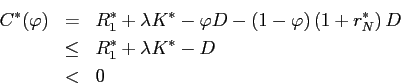
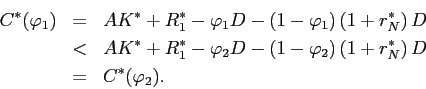
Step 8: To verify the equilibrium, it suffices to show that

$$C^{*}(\varphi)\ge0\;\forall\varphi\in[0,\varphi_{R}^{*}).$$

Since $C^{*}(\varphi)$ is strictly increasing in $\varphi$, it suffices to show $C^{*}(0)\ge0$.

$$\begin{array}[c]{lll} C^{\ast}(0) & = & (A(1-\varphi_{R}^{\ast})+\varphi_{R}^{\ast})D+\frac {G(\varphi_{R}^{\ast})+(1-F(\varphi_{R}^{\ast}))(\lambda+(1-\lambda )\varphi_{R}^{\ast})-(1+r_{W})}{F(\varphi_{R}^{\ast})-G(\varphi_{R}^{\ast} )}D\ & = & (A-1)(1-\varphi_{R}^{\ast})D-\frac{(1-\lambda)(1-\varphi_{R}^{\ast })(1-F(\varphi_{R}^{\ast}))+r_{W}}{F(\varphi_{R}^{\ast})-G(\varphi_{R}^{\ast })}D\ & = & (A-1)(1-\varphi_{R}^{\ast})D-(\sigma+1)\frac{(1-\lambda)(1-\varphi _{R}^{\ast})(1-\varphi_{R}^{\ast})^{\frac{1}{\sigma}}+r_{W}}{1-(1-\varphi _{R}^{\ast})^{\frac{1}{\sigma}+1}}D\ & = & (A-1)\left[ \frac{A-1}{A-\lambda}(\frac{\sigma}{\sigma+1})\right] ^{\sigma}D-(\sigma+1)\frac{(1-\lambda)(\frac{A-1}{A-\lambda}(\frac{\sigma }{\sigma+1}))^{\sigma+1}+r_{W}}{1-(\frac{A-1}{A-\lambda}(\frac{\sigma} {\sigma+1}))^{\sigma+1}}D \end{array}$$

Note that

$\underset{A\rightarrow\infty}{\lim}\left[ (A-1)\left[ \frac{A-1}{A-\lambda }(\frac{\sigma}{\sigma+1})\right] ^{\sigma}-(\sigma+1)\frac{(1-\lambda )(\frac{A-1}{A-\lambda}(\frac{\sigma}{\sigma+1}))^{\sigma+1}+r_{W}} {1-(\frac{A-1}{A-\lambda}(\frac{\sigma}{\sigma+1}))^{\sigma+1}}\right] =+\infty$

Hence $\exists A^{*}(\lambda,\sigma,r_{W})$ such that $\forall A\ge A^{*}$, $C^{*}(0)\ge0$.

PROOF OF PROPOSITION 2:

(i) From Proposition 1, we know that

$\varphi_{R}^{\ast}=1-\left[ \frac{A-1}{A-\lambda}(\frac{\sigma}{\sigma +1})\right] ^{\sigma}\cdot$

Then,

$$\begin{array}[c]{lll} \partial\varphi_{R}^{\ast} & > & 0\ & \Leftrightarrow & \ -\left\{ \log\left[ \frac{A-1}{A-\lambda}(\frac{\sigma}{\sigma+1})\right] +\left. \frac{1}{\sigma+1}\right\} \left[ \frac{A-1}{A-\lambda} (\frac{\sigma}{\sigma+1})\right] ^{\sigma}\right. & > & 0\ & \Leftrightarrow & \ \log\left[ \frac{A-1}{A-\lambda}(\frac{\sigma}{\sigma+1})\right] +\frac {1}{\sigma+1} & < & 0 \end{array}$$

Since $\lambda<1<A$, it suffices to show

$h(\sigma)\equiv\log(\frac{\sigma}{\sigma+1})+\frac{1}{\sigma+1}\leq0$

, which is true since $h(\sigma)$ is increasing in $\sigma$, $\underset{\sigma\rightarrow+\infty}{\lim}h(\sigma)=0^{+},$and $\underset{\sigma\rightarrow0^{+}}{\lim}h(\sigma)=-\infty,$ which implies that $h(\sigma)<0$ for all $\sigma>0$.

(ii) From Corollary 1, we know that

$\Pr\left(\psi=1\right)=1-F\left(\varphi_{R}^{*}\right)$

Substituting for $\varphi_{R}^{*}$, we get

$\Pr(\psi=1)=\frac{A-1}{A-\lambda}(\frac{\sigma}{\sigma+1})$

The result is obvious.

PROOF OF PROPOSITION 3:

Reserves Shortfall  Before writing the planner's problem, it is useful to derive how many countries have to suffer a crisis for a given level of reserves shortfall. Suppose all countries coordinate to set $\varphi_{R}^{C}=\left(\bar{\varphi}-\varepsilon\right)$ reserves aside and invest $\bar{K}+\varepsilon D$¹⁹. The interim shortfall is: $\varepsilon D$.

Some countries will have to (fully) liquidate to pay $1+r_{S}(\epsilon)=\bar{\varphi}+\lambda\bar{K}/D-\left(1-\lambda\right)\varepsilon$ since their normal interim payments cannot be met. Let us denote $\ell\left(\varepsilon\right)$, the measure of countries that face a crisis. We have:

$$1-\ell\left(\varepsilon\right)=F_{\sigma}\left(\widehat{\varphi}\left(\varepsilon\right)\right)$$

where:

$$\bar{\varphi}-\varepsilon=\int_{0}^{\widehat{\varphi}\left(\varepsilon\right)}\varphi dF_{\sigma}\left(\varphi\right)=G_{\sigma}\left(\widehat{\varphi}\left(\varepsilon\right)\right)\quad\Leftrightarrow\quad\widehat{\varphi}\left(\varepsilon\right)=G_{\sigma}^{-1}\left(\bar{\varphi}-\varepsilon\right)$$

So:

$$\ell\left(\varepsilon\right)=1-F_{\sigma}\left[G_{\sigma}^{-1}\left(\bar{\varphi}-\varepsilon\right)\right]$$

The reserves decision $\varepsilon$ determines the probability $\ell\left(\varepsilon\right)$ that a country is in a sudden stop. The shortfall limits the interim insurance since the interim debt repayment of some countries, the ones with the largest shocks, cannot be met. We know:

• $\ell\left(0\right)=0$ and $\ell\left(\bar{\varphi}\right)=1$
• $\ell\left(\varepsilon\right)$ is strictly increasing in $\varepsilon$
• $G_{\sigma}\left(\varphi\right)=\frac{\sigma}{\sigma+1}\left[1-\left(1-\frac{1}{\sigma}\varphi\right)\left(1-\varphi\right)^{\frac{1}{\sigma}}\right]\quad\Rightarrow\quad\ell\left(\varepsilon\right)=\left[1-G_{\sigma}^{-1}\left(\bar{\varphi}-\varepsilon\right)\right]^{\frac{1}{\sigma}}$

We now write the planner's problem as choice of reserves shortfall.

Planner's Problem  Noting that the interim decision has been solved above, the planner's problem is:

$$\begin{array}{cc} \max_{\varepsilon} & C\ \text{subject to} \end{array}$$

$$\left(\bar{\varphi}-\varepsilon\right)D+\left(\bar{K}+\varepsilon D\right)-D \le 0$$ (23)

$$C+\left[\int_{0}^{\widehat{\varphi}\left(\varepsilon\right)}\left(1-\varphi\right)dF_{\sigma}\left(\varphi\right)\right]\left(1+r_{N}\right)D-A\left(1-\ell\left(\varepsilon\right)\right)\left(\bar{K}+\varepsilon D\right) \le 0$$ (24)

$$\ell\left(\varepsilon\right)\left(1+r_{S}(\epsilon)\right)+\int_{0}^{\widehat{\varphi}\left(\varepsilon\right)}\left[\varphi+\left(1-\varphi\right)\left(1+r_{N}\right)\right]dF_{\sigma}\left(\varphi\right)-\left(1+r_{W}\right) \ge 0$$ (25)

$$\left(1+r_{S}(\epsilon)\right)-\left[\left(\bar{\varphi}-\varepsilon\right)D+\lambda\left(\bar{K}+\varepsilon D\right)\right] \ge 0$$ (26)

$$C,\;\epsilon \ge 0$$ (27)

Equations (23) - (27) represent initial resource constraint, final resource constraint, participation constraint, renegotiation proofness, and non-negativity constraint, which are analogous to equations (3), (6), (9), (4) , and (7), respectively. This simplifies to:

$$\begin{array}{cc} \max_{\varepsilon} & C\ \text{subject to} \end{array}$$

$$C+\left[1-\ell\left(\varepsilon\right)-\left(\bar{\varphi}-\varepsilon\right)\right]\left(1+r_{N}\right)D-A\left(1-\ell\left(\varepsilon\right)\right)\left(\bar{K}+\varepsilon D\right) \le 0$$ (28)

$$\ell\left(\varepsilon\right)\left(1+r_{S}(\epsilon)\right)+\int_{0}^{\widehat{\varphi}\left(\varepsilon\right)}\left[\varphi+\left(1-\varphi\right)\left(1+r_{N}\right)\right]dF_{\sigma}\left(\varphi\right)-\left(1+r_{W}\right) \le 0$$ (29)

$$\left(1+r_{S}(\epsilon)\right)-\left[\left(\bar{\varphi}-\varepsilon\right)D+\lambda\left(\bar{K}+\varepsilon D\right)\right] \ge 0$$ (30)

$$C,\;\epsilon \ge 0$$ (31)

Equation (29) can be written as²⁰:

$$\begin{array}{ccc} \ell\left(\varepsilon\right)\left(1+r_{S}(\epsilon)\right)+\left(\bar{\varphi}-\varepsilon\right)+\left(1+r_{N}\right)\left[1-\ell\left(\varepsilon\right)-\left(\bar{\varphi}-\varepsilon\right)\right] & = & \left(1+r_{W}\right)\end{array}$$ (32)

Substituting (32) into (28) yields:

$$C+\left(\left(1+r_{W}\right)-\left(\bar{\varphi}-\varepsilon\right)-\ell\left(\varepsilon\right)\left(1+r_{S}(\epsilon)\right)\right)D-A\left(1-\ell\left(\varepsilon\right)\right)\left(\bar{K}+\varepsilon D\right)\le0$$

The planner's problem can then be written as:

$$\begin{array}[c]{ll} \max_{\varepsilon} & A(1-l(\varepsilon))(\frac{\overline{K}}{D}+\varepsilon )-((1+r_{W})-(\overline{\varphi}-\varepsilon)-l(\varepsilon)(1+r_{S} (\varepsilon)))\ & \Leftrightarrow\ \max_{\varepsilon} & -l(\varepsilon)A\frac{\overline{K}}{D}+A(1-l)(\varepsilon ))\varepsilon-\varepsilon+l(\varepsilon)(1+r_{S}(\varepsilon))+A\frac {\overline{K}}{D}+\overline{\varphi}-(1-r_{W})\ & \Leftrightarrow\ \max_{\varepsilon} & -l(\varepsilon)A\frac{\overline{K}}{D}+A(1-l)(\varepsilon ))\varepsilon-\varepsilon+l(\varepsilon)\left[ \overline{\varphi} +\lambda\frac{\overline{K}}{D}-(1-\lambda)\varepsilon\right] \end{array}$$

This is not a linear problem in $\varepsilon$ since $\ell\left(\varepsilon\right)$ is not linear. However, we know that:

$$\begin{array}[c]{llll} l(\varepsilon) & = & 1-F_{\sigma}\left[ G_{\sigma}^{-1}(\overline{\varphi }-\varepsilon)\right] & \ & \Downarrow & & \ l^{\prime}(\varepsilon) & = & -F_{\sigma}^{^{\prime}}\left[ G_{\sigma} ^{-1}(\overline{\varphi}-\varepsilon)\right] \times\left( \frac{1} {G_{\sigma}^{^{\prime}}\left[ G_{\sigma}^{-1}(\overline{\varphi} -\varepsilon)\right] }\right) \times(-1) & \ & = & \frac{F_{\sigma}^{^{\prime}}\left[ G_{\sigma}^{-1}(\overline{\varphi }-\varepsilon)\right] }{G_{\sigma}^{^{\prime}}\left[ G_{\sigma}^{^{\prime} }(\overline{\varphi}-\varepsilon)\right] } & \ & = & \frac{f\left[ G_{\sigma}^{-1}(\overline{\varphi}-\varepsilon)\right] }{\left[ G_{\sigma}^{-1}(\overline{\varphi}-\varepsilon)\right] f\left[ G_{\sigma}^{-1}(\overline{\varphi}-\varepsilon)\right] } & \text{as }F^{\prime}=f\text{ and }G^{\prime}(\varphi)=\varphi f(\varphi)\ & = & \frac{1}{G_{\sigma}^{-1}(\overline{\varphi}-\varepsilon)} & \ & = & \frac{1}{\widehat{\varphi}(\varepsilon)} & \end{array}$$

The F.O.C. w.r.t. $\varepsilon$ gives:

$-l^{^{\prime}}(\varepsilon)A\frac{\overline{K}}{D}-l^{^{\prime}} (\varepsilon)A\varepsilon+A(1-l(\varepsilon))-1+l^{^{\prime}}(\varepsilon )\left[ \overline{\varphi}+\lambda\frac{\overline{K}}{D}-(1-\lambda )\varepsilon\right] -(1-\lambda)l(\varepsilon)\geq0$

with equality if $\epsilon>0$. Rearranging yields:

$$\begin{array}[c]{ll} -l^{^{\prime}}(\varepsilon)A\left( \frac{\overline{K}}{D}+\varepsilon\right) +A(1-l(\varepsilon))-(1-\lambda)l(\varepsilon)+l^{^{\prime}}(\varepsilon )(1+r_{S}(\varepsilon))-1 & \geq0\ & \Leftrightarrow\ (A-1)-(A+1-\lambda)l(\varepsilon)-l^{^{\prime}}(\varepsilon)\left[ A\left( \frac{\overline{K}}{D}+\varepsilon\right) -(1+r_{S}(\varepsilon))\right] & \geq0\ & \Leftrightarrow\ (A+1-\lambda)F_{\sigma}(\widehat{\varphi}(\varepsilon))-\frac{A\left( \frac{\overline{K}}{D}+\varepsilon\right) -\left( \overline{\varphi} +\lambda\frac{\overline{K}}{D}-(1-\lambda)\varepsilon\right) } {\widehat{\varphi}(\varepsilon)}-(2-\lambda) & \geq0\ & \Leftrightarrow\ (A+1-\lambda)F_{\sigma}(\widehat{\varphi}(\varepsilon))-\frac{A(1-\overline {\varphi}+\varepsilon)-(\overline{\varphi}+\lambda-\lambda\overline{\varphi }-(1-\lambda)\varepsilon)}{\widehat{\varphi}(\varepsilon)}-(2-\lambda) & \geq0\ & \Leftrightarrow\ (A+1-\lambda)F_{\sigma}(\widehat{\varphi}(\varepsilon))-\frac{(A-\lambda )-(A+1-\lambda)(\overline{\varphi}-\varepsilon)}{\widehat{\varphi} (\varepsilon)}-(2-\lambda) & \geq0 \end{array}$$

At $\varepsilon=0$, the L.H.S. of the F.O.C. is:

$$\begin{array}[c]{l} (A+1-\lambda)-\left[ (A-\lambda)-(A+1-\lambda)(\overline{\varphi})\right] -(2-\lambda)\ =(A+1-\lambda)\overline{\varphi}-(1-\lambda)\ >0\text{ iff }\sigma>\frac{1-\lambda}{A} \end{array}$$

Therefore, $\varphi_{R}^{C}=\bar{\varphi}$ if and only if $\sigma\leq\left(1-\lambda\right)/A$. Otherwise, $\varphi_{R}^{C}<\bar{\varphi}$. Obviously, in any case: $\varphi_{R}^{C}\leq\bar{\varphi}$.

Finally, given that $\varphi_{R}^{*}=1-\left[\left(A-1\right)/\left(A-\lambda\right)\sigma/\left(\sigma+1\right)\right]^{\sigma}$ and $\bar{\varphi}=\frac{\sigma}{\sigma+1}$:

$$\varphi_{R}^{*}>\bar{\varphi}\Leftrightarrow\frac{1}{\sigma+1}>\left(\frac{A-1}{A-\lambda}\right)^{\sigma}\left(\frac{\sigma}{1+\sigma}\right)^{\sigma}$$

Since $\lambda<1<A$, it is sufficient to show that:

$$\frac{1}{\sigma+1}>\left(\frac{\sigma}{1+\sigma}\right)^{\sigma}$$

This is always true for $\sigma\in\left(0,1\right)$.

Footnotes

**  Sewon Hur (University of Pittsburgh): [email protected] | Illenin O. Kondo (Federal Reserve Board): [email protected]. We thank Cristina Arellano, Andrew Atkeson, V.V. Chari, Daniele Coen-Pirani, Bora Durdu, Tim Kehoe, Enrique Mendoza, Fabrizio Perri, Marla Ripoll, and John Rogers for many valuable comments. We have also benefited from comments by seminar participants at the University of Minnesota, Washington University in St. Louis, the Society for Economic Dynamics 2011 meetings, the Cantabria Nobel Campus 2012 meetings, the University of Pittsburgh, the Federal Reserve Board, the Midwest Macroeconomics 2012 Fall Meetings, and the Federal Reserve Bank of Minneapolis. The data used in this paper are available online. First draft: September 2010. The views in this paper are solely the responsibility of the authors and should not be interpreted as reflecting the views of the Board of Governors of the Federal Reserve System or of any other person associated with the Federal Reserve System. All errors and shortcomings are ours alone. Return to text

1.  While acknowledging other potential motives for holding reserves such as foreign exchange management (see for example Dooley et al. 2004), we focus on the role of reserves as a buffer (and preventive measure) against sudden stops. This is consistent with the view of policymakers. For example, Ben Bernanke stated that "foreign reserves have been used as a buffer against potential capital outflows" (Bernanke 2005) and a recent IMF survey of reserve managers found that building a "buffer for liquidity needs" was the foremost reason for building reserves (International Monetary Fund 2011).  Return to text

2.  Arellano and Ramanarayanan (2012) and Broner et al. (2007) explore models of debt maturity and why emerging economies issue short-term debt.  Return to text

3.  The dataset stops in 2007 because the external debt liabilities series constructed by Lane and Milesi-Ferretti (2007) stops in 2007. Other data on these emerging economies after 2007 indicates that sudden stops were still rare and reserves remained high compared to the late 1990s. The dataset starts after 1990 because of data availability, especially for current account data. Moreover, financial liberalization in emerging economies was largely still ongoing in the late 1980s, as documented by Buera et al. (2011).  Return to text

4.  Our sudden stop episodes are: Turkey (1994), Argentina, Mexico (1995), Thailand (1997), Czech Republic, Indonesia, Philippines, South Korea (1998), Chile, Peru, Russia (1999), Argentina, Turkey (2001). Durdu et al. (2009) report other episodes: Malaysia (1997), Brazil, Colombia, Pakistan (1999). In any case, there was an outburst in sudden stops between 1997 and 2001. Our methodology for constructing sudden stop episodes is explained in the data appendix.  Return to text

5.  Advanced economies here include the major reserve currencies: France, Germany, U.K., and U.S.  Return to text

6.  We obtain similar results when we separately estimate the model for each variable. The findings are also similar using alternative measures of reserves such as the reserves-to-GDP ratio used by Gourinchas and Obstfeld (2012). We prefer reserves as a fraction of external debt liabilities since it is a measure consistent with our theory.  Return to text

7.  We assume that the foreigners' capital endowment is finite and large enough.  Return to text

8.  This is in contrast to Diamond and Dybvig (1983) who focus on the limits to optimal risk-sharing among creditors that arise from self-fulfilling "panic" runs. More generally, one can allow for both "panic" crises and "rational" sudden stops to occur using a sunspot variable. Our restriction is without loss of generality if crisis payoff for the government is zero as is the case in this section.  Return to text

9.  The assumption that lenders receive zero net return on debt called in the interim is not essential.  Return to text

10.  The sovereign debt literature (see Yue 2010) documents the use of collective action during debt renegotiation.  Return to text

11.  Clearly, to the extent that liquidity shocks are correlated across countries, the i.i.d. case overstates the gains from mutual insurance. Akinci (2012) finds that global factors account for 20 percent of movements in aggregate activity in emerging economies.  Return to text

12.  The superscript $j$ and the subscript $t$ are therefore added to the variables from the previous model to denote the country and the period. We keep the subscripts indicating the stage $s$ when necessary.  Return to text

13.  Alternatively, agents can update their priors using the realized liquidity shocks, $\left\{ \varphi_{t}^{j}\right\} _{j=1,..,N}$. This specification yields similar results with the only noticeable difference being that the speed of learning is faster, and therefore slightly fewer sudden stops in the interim. However, there is still an outburst of sudden stops during the transition. We find it more appealing to have countries learn using sudden stop occurrences around the world instead.  Return to text

14.  For example, estimates for liquidation costs include 30.5 percent (James 2012) and 49.9 percent (Brown and Epstein 1992) in bank failures, and 37 percent (Alderson and Betker 1996) in Chapter 7 liquidations, while Ennis and Keister 2003 use liquidation costs of 60 percent and 70 percent in their analysis. We also run sensitivity analysis with different values of $\lambda$, and find little variation in the main results. See Table A.2 in the appendix for details.  Return to text

15.  The results hold as long as the productivity is sufficiently high.  Return to text

16.  Technically, a planner with a discrete number of countries still faces aggregate uncertainty. The case of a continuum of countries is more tractable and corresponds to an upper bound on the over-accumulation of reserves.  Return to text

17.  Reserves relative to GDP show exactly the same pattern.  Return to text

18.  For computational convenience, we impose that the cutoff rule such that sudden stops occur if and only if $\varphi\ge\varphi_{S}\left(R_{0};\rho\right)$. While this condition was an equilibrium result in the basic model, we cannot analytically prove the cutoff rule in the extended model. The cutoff rule significantly lowers the computational burden. We find that this restriction is not binding in our simulations.  Return to text

19.   $\bar{\varphi}D+\bar{K}=D$ Return to text

20.  This is assuming the shortfall is not too high. Otherwise, the consumption would be negative due to the high interest implied by the high reserves shortfall.  Return to text

This version is optimized for use by screen readers. Descriptions for all mathematical expressions are provided in LaTex format. A printable pdf version is available. Return to text

Home | Economic research and data | Publications and education resources
Accessibility | Contact us
Last update: August 1, 2014