Skip to: [Printable Version (PDF)]

Board of Governors of the Federal Reserve System
International Finance Discussion Papers
Number 1081, June 2013 --- Screen Reader Version*

Capital Flows to Emerging Market Economies: A Brave New World?^**

Shaghil Ahmed and Andrei Zlate

NOTE: International Finance Discussion Papers are preliminary materials circulated to stimulate discussion and critical comment. References in publications to International Finance Discussion Papers (other than an acknowledgment that the writer has had access to unpublished material) should be cleared with the author or authors. Recent IFDPs are available on the Web at http://www.federalreserve.gov/pubs/ifdp/. This paper can be downloaded without charge from the Social Science Research Network electronic library at http://www.ssrn.com/.

Abstract:

We examine the determinants of net private capital inflows to emerging market economies. These inflows are computed from quarterly balance-of-payments data from 2002:Q1 to 2012:Q2. Our main findings are: First, growth and interest rate differentials between EMEs and advanced economies and global risk appetite are statistically and economically important determinants of net private capital inflows. Second, there have been significant changes in the behavior of net inflows from the period before the recent global financial crisis to the post-crisis period, especially for portfolio inflows, partly explained by the greater sensitivity of such flows to interest rate differentials and risk aversion. Third, capital control measures introduced in recent years do appear to have discouraged both total and portfolio inflows. Fourth, in the pre-crisis period, there is some evidence that greater foreign exchange intervention to curb currency appreciation pressures brought more capital inflows down the line, but we cannot identify such an effect in the post-crisis period. Finally, we do not find statistically significant positive effects of unconventional U.S. monetary expansion on total net EME inflows, although there does seem to be a change in composition toward portfolio flows. Even for portfolio flows, U.S. unconventional policy is only one among several important factors.

Keywords: Emerging market economies, capital flows, capital controls, foreign exchange

JEL classification: F3, E5.

1  Introduction

According to economic theory, free movement of capital across national borders is beneficial to all countries, as it leads to an efficient allocation of resources that raises productivity and economic growth everywhere. In practice, however, as now appears to be well recognized, large capital flows can also create substantial challenges for policymakers. These challenges have recently come to the forefront again for emerging market economies (EMEs). After tanking during the global financial crisis of 2008-09, net private capital flows to EMEs surged in the aftermath of the crisis and have been volatile since then, raising a number of concerns in recipient economies.¹ To the extent that the volatility is driven by the fickleness of international investors, it creates a risk of financial instability. Large inflows can also make more difficult the pursuit of appropriate macroeconomic policies to maintain solid economic growth without rising inflation. If, in response, authorities raise policy rates while allowing their currencies to appreciate, this leads to a loss of international competitiveness which could hurt export and growth performance. But if they slow the pace of monetary tightening to deter inflows, or if they resist currency appreciation pressures through intervention, the ability to follow appropriate independent monetary policies is compromised. Such a course of action could result in excessive liquidity and economic overheating, creating vulnerability to boom-bust cycles. And finally, if they resort to capital controls, not only is it an open question how effective these may prove based on the past historical experience, but the use of such controls also risks creating economic distortions that could weigh on economic activity over the longer term.

EMEs appear to have employed a mix of policy responses to try and address these concerns. In response to the sharp rebound in capital flows after the global financial crisis, policymakers allowed some currency appreciation but also intervened in foreign exchange markets to partially stem currency appreciation pressures; several of them introduced some capital controls and macroprudential measures; and they eased somewhat on policy rate increases needed to stabilize their economies. With advanced economies providing powerful monetary stimulus to revive their sluggish economies and the EMEs facing a plethora of capital inflows amid strong recoveries, policy tensions arose between these two groups of economies. Several EMEs argued that the advanced-economy policies, including unconventional monetary expansion in the United States through large-scale asset purchases, were primarily responsible for the excessive flows of capital to their economies and creating adverse spillover effects.

In light of these developments, concerns and policy tensions, our paper considers a number of important questions related to the behavior of private capital flows to EMEs in recent years and the policy responses they have triggered in the recipient economies: (1) What are the main drivers of private capital flows into EMEs? (2) Has there been a sea-change in their behavior from before the global financial crisis to after? (3) Have the latest round of capital control measures introduced in several EMEs since the crisis proved effective in slowing down these inflows? (4) To what extent are capital inflows into EMEs exacerbated in the first place by policies that allow only limited flexibility of the exchange rate? (5) How much has unconventional monetary policy easing in the United States spurred capital flows into EMEs? Despite a substantial amount of recent work on aspects of these issues, the answers to these questions are not settled. Our paper attempts to shed some further light.

The answer to the first question would seem to be crucial in informing the debate about the appropriate policy responses to capital inflows by EMEs. It would be particularly relevant whether such inflows were primarily a result of factors such as international investors' risk appetite, or of economic fundamentals of the recipient countries, including their growth prospects.

The existing literature does not generally favor one determinant over another. Among the more recent studies, Byrne and Fiess (2011) find U.S. interest rates to be a crucial determinant of at least the common component of global capital flows to EMEs.² Similarly, using a panel-data approach, IMF (2011a) finds loose policy in the advanced economies to be an important determinant, but so also are the improved fundamentals and growth prospects of EMEs. Ghosh et al. (2012) identify episodes of capital inflow surges and find a variety of factors to be important in increasing the likelihood of a surge to EMEs, including lower U.S. interest rates, greater global risk appetite, and a particular EME's own attractiveness as an investment destination.³ Focusing on effects of Federal Reserve balance sheet changes on net flows to emerging market-dedicated funds, Fratzscher et al. (2012) find that unconventional monetary policies in the United States have exerted sizable effects on net inflows. But they also conclude that the effects of U.S. unconventional policies have been relatively small compared to other factors. On the other hand, Forbes and Warnock (2012), focusing on gross flows, find no significant role for changes in global interest rates or in global liquidity (as measured by the money supplies of key advanced economies) in affecting surges or stops of foreign inflows; however, like other studies, they do find global risk aversion to be an important and robust factor. Their results, though, are not purely for flows to EMEs, but focus on cross-border inflows into a large sample of countries that includes both advanced and emerging economies. Consistent with the general findings in the literature, our results also point to several factors being important in driving EME capital inflows, namely growth and policy rate differentials as well as global risk appetite. Given this, one contribution of our work is to try to gauge the importance of the different factors for the variability of capital inflows.

Turning to the effectiveness of capital controls, results based on the historical experience prior to 2009 generally suggest that capital controls have been more successful in altering the composition of flows to a country than in changing the aggregate volume, except perhaps in the very short run. (See, for example, Cardoso and Goldfajn, 1998; Cardenas and Barrera, 1997; Montiel and Reinhart, 1999; De Gregorio et al., 2000; Clements and Kamil, 2009; Ostry et al., 2010; and Qureshi et al, 2011).⁴ In a more recent paper, Forbes and Warnock (2012) look at a variety of capital account restrictions and find virtually no effect of such restrictions on cross-border flows. Their sample period goes through 2009, but there is relatively little empirical evidence on the effectiveness or otherwise of the cyclical types of capital controls that several EME have introduced since 2009 in the aftermath of the global financial crisis, which we focus on.

With respect to the question of the role of limited exchange rate flexibility in creating a vicious circle of capital inflows and currency appreciation pressures, some previous studies have also considered the role of exchange rate regimes. For example, the Ghosh et al. (2012) study mentioned earlier finds that while having a more flexible exchange rate regime does not statistically significantly affect the likelihood of a surge in capital flows, conditional on having a surge, it does diminish the magnitude of the surge. The magnitude of the surge is also positively related to their measure of currency undervaluation.⁵ In this paper, we use a direct measure of foreign exchange intervention that has been carefully constructed by Malloy (2013) to examine its importance for EME capital flows in both the pre-crisis and post-crisis period.

Finally, regarding the impact of recent advanced-economy monetary policies on EME capital flows, despite much debate on this topic, there have not been many empirical studies that systematically look at this channel, including isolating the impact of unconventional tools. Most discussions of the impact of monetary expansion in advanced economies are inferred from studies of the effect of long-term U.S. interest rates (or other proxy for global interest rates) on the EME capital flows mostly in the pre-crisis period, and often do not cover the period of the recent unconventional monetary policy as part of their sample period. One important exception is the Fratzcher et al. (2012) study discussed above, which focuses directly on the Federal Reserve's asset purchase announcements and actual balance sheet changes. The effect measured, though, is on flows to EME-dedicated funds, which form only a small part of total capital inflows to these economies. In our paper, unlike in the existing literature, we isolate changes in long-term U.S. interest rates that can be directly attributed to unconventional policies, and then examine the effect of such changes on EME balance-of-payments (BOP) capital flows.

The remainder of this paper is organized as follows. As background, section 2 provides the main properties of capital flows to EMEs over the past decade or so and the policy responses they have elicited in recent years. Section 3 presents the empirical methodology we utilize to answer the five questions posed in this paper, compares this methodology to those of others, and describes the data used in the paper. Section 4 presents our main results, interprets them, and briefly points to some robustness exercises we have done. Section 5 concludes.

2  Main Features of Capital Flows to EMEs and Policy Responses

Figure 1 (top panel) shows the total net private capital inflows into major emerging Asian and Latin American economies since 2002, along with their components by type of investment.⁶ For several years prior to the global financial crisis, these economies received sizable net inflows of private capital. These net inflows turned sharply negative (i.e. to net outflows) at the onset of the crisis. They then surged in the second half of 2009 and 2010 as strong economic recoveries took hold in these economies. But net inflows dried up again in the second half of 2011 with the intensification of the European crisis and the associated rise in global risk aversion, before picking up again as the easing of financial stresses in Europe appeared to improve investor sentiment. Looking at components of the net inflows, foreign direct investment (FDI, the green bars) has been relatively stable over the years, with most of the volatility concentrated in portfolio flows (the blue bars) and banking and other flows (the red bars).⁷

The middle and bottom panels of figure 1 present the gross inflows and the gross outflows, separately. Note that India and Malaysia are excluded in these panels because they report only some of the components of gross flows by investment type.⁸ However, since these two countries' flows are relatively small, the difference between gross inflows in the middle panel and the gross outflows in the bottom panel comes fairly close to the net inflows reported in the top panel. Interestingly, gross outflows mimic a pattern similar to gross inflows - that is, when foreign investors are increasing their holding of EME assets, EME investors are also increasing their holdings of foreign assets. Yet, because these similar movements in gross outflows are generally lower in magnitude, the behavior of net inflows is similar to that of gross inflows with a fairly high correlation. The issue of using net inflows versus gross inflows is a topic of debate in the literature, and we will return to this question in our methodology section.

Figure 2 shows the cumulative net inflows since 2002, which abstracting from valuation changes, can give a sense of how the outstanding amounts of these investments have evolved. A noteworthy feature of the cumulative flows is that the pre-crisis runup in flows was especially concentrated in banking and other investments (the red line), whereas the subsequent collapse during the crisis occurred in both portfolio flows and banking flows. Also, the post-crisis recovery was dominated by portfolio flows (the blue line). Finally, cumulative net inflows of FDI have been much bigger in magnitude than cumulative net inflows of portfolio or banking and other investments.

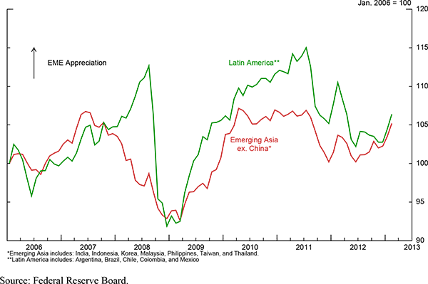
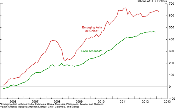
Next we turn to the policy responses in EMEs that these capital flows have elicited. First, as can be seen from figure 3, EME policymakers in both emerging Asia and Latin America allowed their currencies to appreciate some in response to the sharp rebound in capital inflows after the global financial crisis, which resulted in less monetary stimulus than would have occurred under a fixed exchange rate regime. However, EME policymakers did not let exchange rates adjust completely freely. They leaned against currency appreciation through intervention sales of domestic currency in the foreign exchange market, thereby accumulating significant amounts of foreign exchange reserves, especially in the case of emerging Asia, as shown in figure 4.

Intervention generally compromises the ability to follow independent monetary policies. Indeed, EME policymakers appear to have tempered somewhat the policy rate increases that their strong post-crisis recoveries seemed to warrant, for fear that policy rate increases might attract even more inflows and thwart their attempts to stabilize their economies. Figure 5 graphs the aggregate output gaps and real policy rate of a select group of EMEs. The figure illustrates that following their sharp recoveries and amid overheating pressures in 2009 and 2010, authorities started reversing the earlier policy rate increases only with a significant lag. EMEs have also used more macroprudential measures in recent years to strengthen their financial systems and target specific sectors, such as property markets, that may be especially susceptible to asset bubbles.

Finally, a number of countries also employed capital controls seeking to slow capital inflows and currency appreciation pressures. Our paper constructs a database of these recent measures, which we will introduce later. For now, table 1 illustrates the control measures by country, the type of flows being targeted to be restricted, and the type of measure used. Capital controls had long been viewed with disfavor in the official international community. But in recent years, there has been a reassessment in both academic and policy circles of the role of controls in reducing risks associated with capital flows. This reassessment has been led by the IMF, which now supports the use of controls in certain, relatively limited, circumstances: when the domestic currency is not undervalued, when the level of reserves is already adequate, and when the economy is in danger of overheating, so that monetary easing to alleviate capital inflows would be undesirable (see, for example, IMF 2010, 2011a, 2012; Ostry et al., 2011). In laying down these conditions, the IMF emphasizes that controls should not be used to substitute for necessary macroeconomic policy adjustments.⁹

3  Methodology

3.1  Empirical Model

We model net private capital inflows to major EMEs in the emerging Asia and Latin America using quarterly panel data since 2002. We will present estimation results for total net inflows and portfolio net inflows; we were less successful in modeling foreign direct investment and banking and other flows individually. The start date of 2002 allows us to compare the period before the global financial crisis, when flows were also strong, to the surge in capital flows after the crisis. Specifically, the general empirical model, variants of which we estimate, can be written as:

$$\frac{NPI_{it}}{Y_{it}}=\alpha _{0}+\dsum \limits_{i=1}^{n-1}\alpha _{i}D_{i}+\beta ^{\prime }X_{it}+\gamma _{1}RA_{t}+\gamma _{2}CC_{it}+\varepsilon _{it}$$ (1)

The left hand side represents the ratio of net private inflows ($NPI$) - either total or portfolio only - to country $i$ during time period $t$ as a fraction of the country's nominal GDP ($Y$), and $n$ is the number of cross-sections (countries) in the panel. These flows as a share of GDP are modeled as a function of fixed effects ($D_{i}=1\$if an observation pertains to country $i$, 0 otherwise), a vector of variables that are likely to influence return differentials ($X$) (that are discussed in more detail below), a measure of global risk aversion ($RA$) that does not vary across countries and thus has no $i$ subscript, and a variable capturing the number of capital control measures ($CC$). The $\alpha$'s, the vector $\beta$, $\gamma _{1}$, and $\gamma _{2}$ represent parameters to be estimated, and $\varepsilon _{it}$ is the unexplained portion of the variation in capital inflows for country $i$ during period $t$.

The most important return differentials driving flows of net foreign investment to the EMEs are generally found to be those between the EMEs and the advanced economies. In addition, returns to foreign investors will be positively influenced by expected appreciation of the currency of the country in which they are investing. Our stance here is that expected appreciation is difficult to measure directly, but that intervention activities systematically aimed at keeping currencies from appreciating increase the expected rate of currency appreciation down the line, and thus are likely to induce capital inflows. Accordingly, return differentials in our empirical work are assumed to be related to the following variables:

$$X_{it}=\left( \begin{array}{c} X_{1it} \\ X_{2it} \\ X_{3it} \\ X_{4it} \end{array} \right) =\left( \begin{array}{c} g_{it}-g_{t}^{AE} \\ R_{it}-R_{t}^{US} \\ \dsum \limits_{k=1}^{8}INTV_{i,t-k}/Y_{it} \\ USLSAPS_{t} \end{array} \right)$$ (2)

where $g_{i}$ and $g^{AE}$ represent, respectively, real GDP growth in country $i$ and in an aggregate of the advanced economies; $R_{i}$ and $R^{US}$ represent the monetary policy rates in country $i$ and in the United States, respectively; $INTV_{i,t-k}$ measures foreign exchange intervention undertaken by country $i$, $k$ quarters ago, with positive values indicating intervention to contain currency appreciation pressures (leading to accumulation of foreign reserves), and negative values indicting intervention to curb currency depreciation pressures (leading to decumulation of foreign reserves). Thus, the first three variables assumed to affect return differentials are the economic growth differential between a given EME and an aggregate of advanced economies, the policy rate differential between a given EME and the United States, and the amount of intervention undertaken on net over the past 8 quarters as a share of GDP. Intervention is expressed as a share of GDP because the dependent variable also expresses net capital private inflows as a share of GDP. Note that we have used a policy differential with the United States only, rather than with the AE aggregate, because most discussions of the impact of AE policies on EME capital flows focus primarily on U.S. policies, and U.S. interest rates are also used generally as a proxy for global interest rates in the empirical work. However, in practice, it makes little difference if the U.S. policy rate is substituted by an aggregate AE policy rate.¹⁰ In addition to these three variables, in the post-crisis period when the lower bound of zero on the U.S. policy rate has been binding, return differentials are also generally expected to be influenced by unconventional U.S. monetary expansion. Accordingly, we also include a variable designed to capture the effects of U.S. Large-Scale Asset Purchases (LSAPs), $USLSAPS$.

Based on (1) and (2), the empirical model can be expressed as:

$$\frac{NPI_{it}}{Y_{it}} = \alpha _{0}+\dsum \limits_{i=1}^{n-1}\alpha _{i}D_{i}+\beta _{1}(g_{it}-g_{t}^{AE})+\beta _{2}(R_{it}-R_{t}^{US})+\beta _{3}\left( \dsum \limits_{k=1}^{8}INTV_{i,t-k}/Y_{it}\right) \notag$$ (3)

$$+\beta _{4}USLSAPS_{t}+\gamma _{1}RA_{t}+\gamma _{2}CC_{it}+\varepsilon _{it}$$

3.2  Comparison With Earlier Methodologies

Much of the previous literature on the determinants of capital flows to EMEs, such as Ghosh et al.(2012) and Forbes and Warnock (2012) mentioned above, has focused on identifying "surges" and "sudden stops," the presumption being that times of unusual flows are different from normal times and may have different determinants.¹¹ While this seems to be a reasonable strategy, it has the downside that it does not easily allow us to see how much of the unusual flows is a result of outsized movements in the explanatory variables that influence these flows in normal times as well, and how much truly cannot be explained by models that apply during normal times. Moreover, with the periods of unusual flows being, by definition, much less common than periods of normal flows, it is difficult to identify how the determinants of capital flows may have changed over time when considering only surges and stops. Yet one of the key questions with respect to recent EME capital flows is whether the resilience of these economies through the global crisis has led to a new world in terms of what is driving these flows. We, therefore, want to investigate how far we can get with the more traditional approach of estimating the same model irrespective of the size of the flows, but looking for structural breaks at different times.

Another point of debate in the literature is whether focusing on gross capital inflows (featuring actions of non-resident investors only) or net inflows (which also take into account the action of domestic residents in foreign markets) is more appropriate, and whether it makes any difference to the results. For example, in the Forbes and Warnock (2012) study, the authors argue that the distinction is material because episodes of surges measured by net inflows - the usual practice in the literature - result, in fact, both from cases of sharp retrenchments by domestic investors of their investments abroad, as well as from cases of genuine surges of investment into the country by foreign investors. As indicated earlier, we do not identify surges or retrenchments, but instead look at investment flows during all times, and our earlier discussion of the behavior of gross versus net flows for the economies we are studying suggests that the pattern of gross vs. net capital inflows is similar. Conceptually, whether to focus on net inflows or gross inflows would seem to depend on the particular question at hand. Thus, net inflows may be more relevant for exchange rate appreciation and general overheating concerns, whereas gross flows may be more relevant for financial stability issues and the capacity of EME financial systems to effectively intermediate the flows. Given the issues we are interested in, we report results on net inflows as our core results, but as part of our robustness checks, we discuss in the Appendix how the results differ if instead we use gross inflows.¹²

The set of countries used also differs across studies of cross-border flows of capital. As we mentioned earlier, Forbes and Warnock (2013) use a mixture of advanced and emerging market economies, but for the set of issues at hand we would want to focus on the EMEs only. Other papers discussed before (for example, Ghosh et al., 2012; Fratzcher et al., 2012; Byrne and Fiess, 2011; and IMF, 2011a) use a mixture of EMEs. The issues we are mainly interested in, however - such as concerns about real exchange rate appreciation pressures, spillover effects of advanced-economy expansionary policies, the effectiveness of recent capital controls - would seem to apply with particular force to the emerging Asian and Latin American EMEs. A very different set of considerations and issues applies to eastern European economies, for example. Even within the Asian EMEs, important world financial hubs like Hong Kong and Singapore have much larger gross capital inflows and outflows, a large portion of which may not be influenced by the same variables that are relevant for other EMEs. Accordingly, in our benchmark results we focus our analysis on emerging Asian and Latin American economies, excluding Hong Kong and Singapore. The economies we include are some of the largest recipients of private capital inflows among emerging markets. In our robustness results (reported in the Appendix), we also study what implications that including other EMEs, such as those in eastern Europe, has for our results.

In discussing our methodology, we also want to raise the issue of whether to include fixed effects or not. It would seem natural to do so, but one relevant consideration is that there are also long-lasting growth differentials between EMEs and AEs that arise from their long-term growth potentials being different. To the extent that such differences are more or less constant over time, but may differ from country to country, they would likely show up in fixed effects and diminish the importance of the growth differential variable. So, one interpretation of fixed effects could be that they are capturing long-lasting growth differentials between countries. On the other hand, anything else that is different between countries that does not vary over time but that affects capital flows to them would also show up in the fixed effects. Based on these considerations, we present both models that include and do not include fixed effects.

Finally, in contrast to our paper, some other studies approach the issue of the determinants of capital flows by first isolating the common component of such flows across countries. Byrne and Fiess (2011) do this in the context of emerging markets, by first identifying the common component of EME capital flows, and then by studying whether this common component has a stochastic trend and what are its determinants. They also find a significant role for human capital and the quality of institutions in driving capital flows.¹³

3.3  Data and Measurement

Our core results are based on a balanced, quarterly panel data set that covers 12 EMEs from emerging Asia and Latin America over the period 2002:Q1 to 2012:Q2. This sample period covers not only the global wave of capital flows from before the 2008-09 crisis (see IMF, 2011a), but also the post-crisis surge through mid-2012. We have discussed in the methodology section above our rationale for focusing on EMEs from these regions. The EMEs included are seven Asian economies (India, Indonesia, Korea, Malaysia, the Philippines, Taiwan and Thailand) and five Latin American ones (Argentina, Brazil, Chile, Colombia and Mexico). The basic sample excludes China, for which quarterly balance of payments (BOP) data are not available prior to 2010; as discussed earlier, it also excludes Hong Kong and Singapore, whose capital flows are not determined by the usual EME considerations, given their status as financial centers. However, for the robustness checks, details of which are in the Appendix, we use an extended sample of 28 EMEs from Asia (including China, Hong Kong and Singapore), Latin America, and emerging Europe.

3.3.1  Capital Flows and Macroeconomic Indicators

To construct the dependent variables, we use quarterly BOP data on net private capital inflows expressed in nominal U.S. dollars and normalized by the quarterly nominal GDP of the recipient economy. In separate specifications, our dependent variables are the total net flows and, alternatively, the portfolio net flows, each normalized by GDP.¹⁴

Turning to explanatory variables, the economic growth differential is measured as the difference between four-quarter real GDP growth rates in each EME and an aggregate of advanced economies.¹⁵ As shown in Figure 6 (top panel), aggregate real GDP growth in EMEs (the red line) has consistently outpaced that in the advanced economies (the blue line), and the growth differential (the orange bars) has fluctuated over the sample period. Note that the growth differential widened in late-2009 and early-2010, reflecting the faster pace of recovery from the crisis in the EMEs. However, as the EMEs slowed more recently, the growth differential narrowed, although it remains sizeable.

The policy interest rate differential is computed as the difference between the nominal policy rate for each EME and the U.S. Federal Funds rate. As shown in Figure 6 (middle panel), the interest rate differential (the orange bars) has been positive, but fluctuated notably over the sample period. During the post-crisis recovery, the differing cyclical positions of the EMEs and advanced economies called for different monetary policy settings, and drove up the interest rate differential. However, over the past several quarters, several EMEs have been lowering policy rates, leading to some narrowing of the interest rate differentials.

As an indicator of global risk appetite or the lack thereof, we use the quarterly average of the Volatility Index (VIX) computed by the Chicago Board Options. This is a measure of the implied volatility of the S&P 500 index, and serves in our regressions as a proxy for the combination of perceived risk and risk aversion. Indeed, Figure 6 (bottom panel) shows that the flows to emerging market-dedicated funds (the red line) have been correlated with the VIX index (the blue line, plotted on an inverted scale so that a movement in the upper direction represents more appetite for risk and less risk aversion). Thus, capital flows to EMEs plunged during the investor panic after Lehman Brothers in 2008, and again as the European situation worsened in the second half of 2011 and in May 2012.¹⁶

Summary statistics on these explanatory variables are provided in table 2.¹⁷

3.3.2  Capital Control Measures

We construct a novel database for the new measures attempting to control capital inflows introduced since the global financial crisis by the EMEs in our sample. We have compiled these measures from local press releases and news bulletins since 2009. We have already mentioned table 1, which illustrates these measures by country, according to the type of inflows targeted and the type of measures used. To give a bit more detail here, among the measures restricting portfolio inflows, taxes on investments by foreigners apply either to the total volume of inflows (Brazil), or to the foreign investors' income from holding local government bonds (in Korea and Thailand). Restrictions on asset holdings include a minimum holding requirement in Indonesia on the short-term bills issued by the central bank.¹⁸ To restrict banking inflows, countries have used taxes on short-term external borrowing or limits on banks' exposure to foreign exchange derivatives, which seek in part to reduce the short-term external debt that banks would use to hedge these derivatives. Finally, a number of EMEs have increased the required reserves on banks' liabilities denominated in foreign currencies.¹⁹

Keeping track of the measures to control capital inflows introduced by the economies in our sample since 2009 - with five of the 12 EMEs having introduced such measures - we construct two types of variables, shown in Figure 7. First, we use the cumulative number of measures in place in any given quarter (the blue/solid lines). Second, we also use the number of new measures introduced in any given quarter (the red/dashed lines), which is the first difference of the number of measures in place.²⁰ As an example, in Brazil, authorities introduced new measures in 2009:Q4 (when the IOF tax was reinstated on foreign investment in both equity and fixed income) and again in 2010:Q4 (when the IOF on fixed income and mutual fund investments was raised twice, and was also extended to derivatives). The IOF on mutual fund investments was lowered in late 2010, but authorities then raised the unremunerated reserve requirements on banks' short dollar positions, and imposed and raised the IOF on banks' short-term external loans in 2011:Q2 and 2011:Q3.²¹

3.3.3  Foreign Exchange Intervention

To study the effect of foreign exchange (FX) intervention on capital flows, we use data on central bank FX intervention that are constructed by Malloy (2013). He compiles the degree of intervention either from published reports provided by certain EMEs on their intervention activities or, if such reports are not available, from monthly changes in central bank reserves adjusted for exchange rate valuation effects. Positive values reflect purchases of foreign currency and thus intervention to prevent currency appreciation. The data are available for nine of the 12 EMEs in our core sample (Argentina, Chile and Malaysia are excluded).²²

3.3.4  Large Scale Asset Purchases (LSAPs)

We use several measures to assess the effect of unconventional U.S. monetary policy on capital flows to EMEs. First, we use indicator variables to assess whether the behavior of flows is unusual during the initial announcements and the implementation periods of the first two rounds of large-scale asset purchases (LSAP) by the Federal Reserve. The indicator variable is equal to 1 for quarters when the programs were first announced or when the amount of purchases was extended, using the standard announcement dates documented by the literature (see Gagnon et al., 2011, Krishnamurthy and Vissing-Jorgensen, 2011, and Bauer, 2012). The " implementation'' indicator variable is equal to 1 for the duration of each program. Second, we use the yields on 10-year U.S. treasury bonds to try to capture the effect of unconventional monetary easing. Third, we use net asset purchases by the Federal Reserve from 2003:Q1 to 2012:Q2 as an instrumental variable to try to isolate more directly the change in Treasury yields that could be attributed to unconventional U.S. monetary policy.²³

4  Core Results

4.1  The Basic Model

We first estimate a basic model without the foreign exchange intervention and capital control variables, separately for the pre-crisis and post-crisis periods. The intervention data are only available for a subset of our countries, and our database does not cover cyclical capital controls before the crisis. Since one of our goals is to compare the pre-crisis to the post-crisis flows, we start off with a model with the same variables over the two periods.²⁴ The empirical models focus on explaining both total and portfolio net capital inflows. However, we do not estimate the model separately for the FDI or the banking and other flows components. FDI flows have been relatively stable, and banking flows are influenced by many additional factors, such as advanced economy regulations, leverage, and banking sector equity (see Brookings, 2012 and Bruno and Shin, 2013b).

Table 3 presents the results of the basic model with total net inflows and portfolio net inflows, both expressed as a percent of GDP, as the alternative dependent variables. As described earlier, the real GDP growth differentials, the policy rate differentials (both expressed in percentage points), and global risk aversion (as measured by the VIX index) are the explanatory variables. The pre-crisis sample period is 2002:Q1 to 2008:Q2, ending just before the collapse of Lehman Brothers, and the post-crisis period is 2009:Q3 to 2012:Q2, with the start date of this period corresponding to the quarter by which flows had definitively recovered from their weakness during the crisis.²⁵ Both simple OLS estimates and estimates with fixed effects (FE) are provided.

In general, the explanatory variables come in statistically significant and with the expected sign, and the magnitudes of the estimated effects appear to be economically significant as well.²⁶ In both the pre-crisis and post-crisis period, the main determinants of total net inflows (columns 1-4) are the growth differentials and policy rate differentials, whereas risk aversion does not come in statistically significant. A one percentage point increase in real GDP growth differentials is associated with additional total net private inflows of 0.3 to 0.5 percent of GDP, with the effects about equal for the pre- and post-crisis periods. A one percentage point increase in the policy rate differential, when statistically significant, is associated with additional total net inflows of 0.2 to 0.7 percent of GDP, with the lower end of the range applying to the pre-crisis period and the upper end of the range applying to the post-crisis period.

The story of the determinants of portfolio net inflows is somewhat different (columns 5-8). Unlike in the case of total net inflows, global risk aversion plays an important part in explaining portfolio flows. As we would expect, greater global risk aversion, measured as an increase in the VIX index, has a negative effect on net portfolio inflows, and the effect is generally statistically significant. Policy interest rate differentials still matter for the models without FE, with a one percentage-point increase in this differential raising net portfolio inflows by 0.16 percent of GDP in the pre-crisis period and by about twice as much, 0.34 percent of GDP, in the post-crisis period. Once FE are included, the importance of the policy rate differential diminishes in terms of statistical significance. Growth differentials appear to be much less important for portfolio inflows than they were found to be for total inflows, especially in the FE model. The diminished significance of growth and interest rate differentials when FE are included is consistent with the idea that these fixed effects may partly be capturing the long-standing growth potential and the long-run interest rate differentials between EMEs and AEs.

The previous literature often divides variables driving the capital flows to EMEs into the so-called "pull" and "push" factors. The variables related to the EMEs themselves are regarded as factors "pulling" flows into these economies, while the rest of the world variables are considered factors "pushing" capital flows into these economies. The usual interpretation seems to be that "push" brings in the problematic kind of flows, while "pull" brings in the acceptable kind. We are not especially fond of this distinction. For example, whether growth differentials widen because foreign growth is low or EME growth is high, in both cases it is economic fundamentals at work driving the flows, which should not be a cause for alarm.²⁷ In any case, the F-statisics reported at the bottom of table 3 suggest that the null hypothesis - according to which the EME and AE growth effects and the EME and U.S. policy rate effects, respectively, are jointly equal in magnitude but of opposite signs - cannot be rejected. As such, in what follows we proceed with the model expressed in growth and policy rate differentials. However, to compare our results to those from other studies, the robustness results in the Appendix present estimates for which the growth and policy differentials are separated into the individual variables that make up the differential.

In general, our results so far support the previous literature (discussed earlier) that finds, on balance, a variety of factors to be important in influencing capital flows to EMEs.

4.1.1  How Important are the Different Drivers?

The coefficients given in table 3 by themselves do not directly tell us the economic importance of the different variables implied by the estimated model. One way to gauge the economic importance of a particular variable is to compare the fitted value from the full model with the model prediction under the counterfactual that keeps the variable of interest at its initial value, rather than allowing it to evolve as it did in reality. Figure 8 reports the results of this exercise for the total net inflows model, for both the pre-crisis period and the post-crisis periods, using the FE model. For the pre-crisis period, the figure shows that if the policy rate differential had been kept constant at its initial value, it would have made little difference to the predicted value of the total net capital inflows, suggesting that policy rate differentials were not an economically important driving force behind the total net inflows. In contrast, if the growth differential or VIX variables were kept constant, this makes a substantial difference to the predicted values, suggesting that these two variables were economically more significant. In the post-crisis period, all three variables appear to matter quite a bit, with their economic importance roughly equal.

Figure 9 presents the corresponding results for the model with net portfolio inflows. In both periods, global risk aversion appears to the most important factor, while the growth and policy rate differentials appear to matter relatively less, especially in the pre-crisis period.

4.1.2  How Different is the Post-Crisis Period From the Pre-Crisis Period?

Alarm bells were ringing particularly loud with respect to surges of capital flows to EMEs in the late 2009 and 2010 period, with some arguing that this was another particularly acute example of the volatility of capital flows problem. Others, however, were arguing that, after having proved their relative resilience to the global financial crisis, the EMEs were entering a brave new world where capital flows may be permanently higher, largely driven by macroeconomic fundamentals.²⁸ With our sample period going up to 2012:Q2, our data set allows us to examine more systematically if and how the post-crisis period differs from the pre-crisis period.²⁹

We begin by asking if the post-crisis behavior of net inflows would be considered unusual relative to what the FE models estimated over the pre-crisis period would predict, given the actual evolution of the determining variables. Figure 10 presents the results, with the flows converted into billions of U.S. dollars (from shares of GDP) and cumulated to provide a clearer picture of their evolution. For the total net inflows model, shown in the left panel, after the crisis, the actual cumulative net inflows (the green line) have been growing at a consistently faster pace than the pre-crisis model would have predicted (the orange line). This can be seen by the slope of the green line being greater than the slope of the orange line in the post-crisis period. Initially, the higher-than-predicted growth rate was just making up for the greater-than-expected loss of flows that occurred during the crisis, but although these losses had been overcome by around late-2010, cumulative flows continued to rise at a faster pace. Thus, there is some evidence of acceleration of total net inflows relative to what the pre-crisis model would predict.

The evidence of acceleration relative to the pre-crisis model prediction (using the FE model) is much stronger for portfolio flows. Interestingly, for cumulative portfolio flows, the model is able to account for the fall during the crisis period. Risk aversion is an important variable in the pre-crisis model, and it also rose sharply during the crisis, which accounts for this result. However, the pre-crisis period model would have predicted cumulative flows to remain subdued in the post-crisis period, whereas actual cumulative flows took off.

In sum, total cumulative net inflows have been somewhat higher in the post-crisis period than the pre-crisis model would have been predicted, but the sea-change appears to be in the behavior of cumulative net portfolio inflows. One possibility might be that flows have simply become less able to be explained by the variables in the model, but the $R^{2}$ values from the FE regressions do not support that. On the contrary, the fits of both the total inflows model and the portfolio inflows models have increased in the post-crisis period.

Another possibility is that the sensitivities to the determining variables have changed from before the crisis to after the crisis, and table 4 presents some structural break tests to asses this. Essentially table 4 re-estimates the model presented in table 3 earlier in such a way that the hypothesis that the effects of the explanatory variables have changed in the post-crisis period can be easily tested. This is done by introducing interaction terms of the explanatory variables with a post-crisis dummy variable. The first three rows reproduce the estimates of the pre-crisis period in table 3; the next three rows represent the difference between effects in the post-crisis period and those in the pre-crisis period. (If we add these effects to the corresponding effects in the first three rows, we will get the total effect for the post-crisis period reported in table 3.)

Consider first the structural break tests for the total net inflows model and the differences in the post-crisis period. The policy rate differential has much bigger effects in the post-crisis period compared to the pre-crisis period, although the difference is statistically significant only for the OLS model (column 2). For the FE model, which was used in figure 10, while a percentage point increase in the policy rate differential in the pre-crisis period would enhance net total inflows by a negligible amount, in the post-crisis period, the effect would be 0.7 percent of GDP. This appears to be the main reason behind flows being stronger than the pre-crisis model would predict.

For the portfolio flows model, the sensitivity to policy rate differentials increases statistically significantly in the post-crisis period (column 4), again from a negligible effect in the pre-crisis period to a 0.6 percent of GDP effect in the post-crisis period. The sensitivity to risk aversion also goes up in magnitude (by about 70 percent) for the post-crisis period. The difference from the pre-crisis period is statistically insignificant, although economically large.

On balance, we would conclude that there have been some structural changes in the sensitivities of flows to policy rate differentials and to risk aversion that do make the post-crisis period different from the pre-crisis period, with the implications for portfolio flows for the two periods being especially stark. But the changes are not always precisely enough determined to be statistically significant.

4.2  The Extended Model

4.2.1  Capital Controls

Table 5 presents the results of adding the capital control variables we have constructed for the post-crisis period to the basic model. Recall that these variables are, alternatively, the number of capital control measures in place every quarter and the contemporaneous and lagged number of new capital control measures introduced every quarter.³⁰

The results suggest that the new capital control measures introduced since 2009 have exerted a significant dampening effect on inflows. Specifically, the number of capital control measures in place variable has a negative and statistically significant coefficient for both total flows (columns 1-2) and portfolio flows (columns 5-6).³¹ In addition, the number of new measures introduced every quarter also have negative and statistically significant effects on capital inflows, although these effects occur with a bit of a lag (columns 3-4 and 7-8).³² The introduction of these capital control variables does not take away from the importance of the growth and interest rate differentials as well as VIX that were reported earlier in table 3.³³ Note that the capital controls did not prevent a surge of flows in the post-crisis period, but the results suggest that flows would have been even higher in the absence of these controls.

The lagged relation between new capital controls and capital flows is consistent with the findings in existing literature suggesting that investors take time to adjust their portfolios (see Forbes et al., 2012). In addition, since our database only includes the original capital control measures - and not the subsequent measures introduced to close loopholes - the lagged relation between controls and flows also suggests a weaker effect initially, but which becomes stronger as loopholes are effectively closed over time.

4.2.2  Foreign Exchange Intervention

Table 6 reports the results for the effect of foreign exchange (FX) intervention by EME central banks on net capital inflows in the pre-crisis period. Recall that our variable measures the cumulative intervention undertaken over the previous two years (i.e. quarters $t-1$ to $t-8$). The use of intervention over the previous two years helps to overcome the endogeneity problem that might arise due to EMEs intervening contemporaneously in response to strong capital inflows.³⁴ Our results indicate that lagged FX purchases had a positive and statistically significant effect on capital inflows during the pre-crisis period, for both total and portfolio net flows. Specifically, $1 billion of intervention brought in about $0.2 billion of portfolio net inflows and about $0.45 billion of total net inflows. The results are consistent with the view that the undervaluation of some EME currencies resulting from FX purchases generates greater expectation of future currency appreciation, thereby increasing expected return differentials in favor of EMEs and enhancing capital flows to these economies.³⁵

For the post-crisis period (not reported), we could not identify any strong effect that intervention brought in significantly more inflows down the road. We attribute this to several factors. First, the crisis period was unusual, and the use of lagged FX intervention over the past two years means that intervention from the crisis period would be used to inform about flows during the post-crisis period. But in the crisis period, intervention was either low or skewed toward FX sales to prevent currency depreciations, while the net inflows to EMEs rebounded quite quickly after the crisis, which tends to create a negative correlation between the two variables. Second, if to address this issue we cut the start of the post-crisis sample period by two years, this leaves too few observations even with a panel setting, to get meaningful estimates. Third, the data suggest significant correlation between FX intervention and some of the other explanatory variables in the post-crisis period, such as capital controls, making it difficult to isolate the effect of intervention by itself. Notably, as shown in column 5 of table 6, even after taking into account a time trend in the number of capital controls in place and fixed effects, FX intervention in the past to stem currency appreciation pressures tends to be followed by the imposition of capital controls, with this effect being statistically significant. This result is consistent with the notion that FX intervention encouraged capital inflows to EMEs, in turn forcing countries to introduce capital controls to discourage these inflows. But it is also consistent with the idea that in response to expectations of large capital inflows, countries use a variety of measures, including first direct FX intervention followed by capital controls.

4.2.3  Unconventional U.S. Monetary Policy

After policy interest rates had reached the zero lower bound and with their economic recoveries still fragile, a number of AE central banks, including the Federal Reserve, resorted to unconventional monetary expansion in efforts to continue to boost economic activity. It is important to emphasize that these unconventional monetary policies are just another form of monetary easing, made necessary because of hitting the zero lower bound on the policy rate; these policies work much through the same channels, by affecting interest rates in the economy to which private spending is sensitive. Indeed, there is some evidence that such unconventional policies in the U.S. lowered yields on U.S. long-term Treasury bonds and similar securities (see D'Amico and King, 2013, D'Amico et al., 2012, and Gagnon et al., 2011). In turn, it has been suggested that lower yields on longer-term U.S. securities may have encouraged capital flows to EMEs (see Fratzcher et., 2012, and IMF, 2011a). We provide some new evidence on this, using several variables related to U.S. LSAPs.

First, table 7 presents results from the inclusion of LSAP indicator variables that were mentioned earlier and are shown in figure 11. These indicator variables are equal to 1 for the quarters in which LSAPs are initially announced and the quarters during which LSAP programs are still in place. In addition to this variable, the models include the earlier growth differential, policy rate differential, and risk aversion variables (but with interaction terms for the crisis- and post-crisis periods), as well as capital controls in place. Note that the crisis period has been included in these regressions, unlike those reported earlier. This is because the first round of LSAPs began during the crisis, and the variation of LSAPs over the sample this provides seems to be necessary to determine their effects on capital flows more precisely. Turing to the specific results in table 7, as we found before, the sensitivity of capital flows to policy rate differentials appears to be higher during the post-crisis period. Interestingly, for the crisis period, the interaction coefficient on the growth differential is negative and about the same in magnitude as the growth differential coefficient for the pre-crisis period, suggesting that the growth differentials ceased to be a determinant of capital flows during the crisis period. With respect to unconventional U.S. monetary policy, the coefficients on the indicator variables for LSAP announcements and implementation are not statistically significant for the total net inflows (columns 1-4), but are positive and statistically significant for the portfolio net inflows (columns 5-8).³⁶

These results suggest that LSAPs changed the composition of EME net capital inflows toward portfolio flows, an issue which we now investigate further. To do so, we first directly include the 10-year Treasury bond yield among the explanatory variables, along with the other variables (see columns 1-2 and 5-6 of table 8). Again, we do not find the Treasury yields to have a statistically significant effect on the total net inflows, but the coefficient of the yield variable in the portfolio investment equation is statistically significant and negative. During the crisis period, the effect of Treasury yields on portfolio flows appears larger, as the slope interaction coefficient is negative and statistically significant. This suggests that the first LSAP program initiated during the crisis - which coincided with net capital outflows from the EMEs - helped to contain some of the portfolio outflows from EMEs. During the post-crisis period, the effect of U.S. Treasury yields on portfolio investment equation is still negative; the positive slope interaction term indicates that the effect is smaller than in the pre-crisis period, but this interaction term is not statistically significant. The results are consistent with the existing literature showing that U.S. Treasury yields have affected capital flows to EMEs in significant ways (see, for example, IMF, 2011a). However, we find no evidence that the effect of Treasury yields has been more pronounced in the post-crisis period than in the pre-crisis period.

U.S. Treasury yields, of course, are also affected by factors other than U.S. monetary policy actions. In an attempt to isolate more directly the effects of unconventional monetary policy on Treasury yields, we use the LSAPs undertaken by the Federal Reserve as an instrument to compute the change in the U.S. 10-year bond yield that could be attributed to the unconventional U.S. monetary policy. Specifically, we first regress the yields (in percentage points) on asset purchases one quarter ahead (in billions of U.S. dollars) over the interval from 2003:Q1 to 2012:Q2. (These two variables are shown in figure 12.) The one-quarter ahead value of asset purchases, rather than the contemporaneous value, fits better, which perhaps is not surprising given that LSAPs are anticipated to some degree and announcements precede the actual purchases.³⁷ Next, we use the difference between the actual yield and what the yield would have been without LSAPs as representing the effect of LSAPs on the yield. As can be seen from columns 3-4 of table 8, total net EME capital inflows do not appear to be statistically significantly affected by the yield changes related to LSAPs, but portfolio flows (columns 7-8) are negatively and statistically significantly affected, once again suggesting that LSAPs have affected the composition of flows. Specifically, a 10 basis point-reduction in the Treasury bond yields related to LSAPs is associated with enhanced net portfolio capital flows to EMEs of about 0.2 percent of the recipients' GDP. The results on the other variables are pretty similar to those reported in table 7.

4.2.4  Robustness Checks

To facilitate an easier comparison with other studies in this literature, we examined the robustness of our results to several alternative specifications. These include separating out the EME and advanced-economy growth differentials into the individual growth rates and policy rates, adding smaller countries in emerging Asia and Latin America, adding emerging European countries as well and allowing regional effects, using Credit Suisse's global risk appetite index (GRAI) instead of VIX, and focusing on gross inflows rather than net inflows. Most of the results were fairly robust qualitatively, but some important quantitative differences could be observed. These robustness results are discussed in detail in the Appendix to this paper.

5  Conclusions

We conclude by giving the answers to the questions we posed that are suggested by our empirical work.

First, consistent with the evidence presented in previous studies, we find net capital flows to EMEs to be determined in the expected manner and statistically significantly by a number of different factors, including growth differentials, policy rate differentials, and global risk aversion. In terms of the economic importance of these factors, in the post-crisis period all three appear to be equally important for both total net inflows and portfolio net inflows, whereas in the pre-crisis period growth differentials were relatively more important for total inflows while risk aversion was relatively more important for portfolio inflows.

Second, we find that there have been some important and significant changes in the behavior of capital flows to EMEs from before the crisis to after. If we apply the pre-crisis model to the post-crisis behavior of the determining variables, the model somewhat underpredicts total net capital inflows, but vastly underpredicts portfolio net inflows. However, these results are not due to an increase in inherent instability of the flows, but due to changes in the sensitivity of the flows to some of the explanatory variables. Primarily, the sensitivity of portfolio flows to policy rate differentials and to risk aversion appears to have increased during the post-crisis period.

Third, using a novel data set that we constructed of capital control measures that several EMEs have used in recent years, we find that these measures appear to have had some effect in dampening capital inflows to these EMEs. While some case studies reach similar conclusions, we are not aware of any previous cross-country study that looks at these effects for the latest capital controls introduced since mid-2009.

Fourth, our results from the pre-crisis period strongly suggest that when countries step up their foreign currency intervention to counter currency appreciation pressures, this intervention tends to be followed by stronger inflows of capital. This is consistent with the idea that such interventions create expectations of future currency appreciations that induce more capital inflows. However, we cannot identify such an effect in the post-crisis period. Some preliminary results suggest that this may be because of the correlation of the intervention variable with other important determinants of flows, such as capital controls, in the post-crisis period.

Finally, we do not find statistically significant effects of unconventional U.S. monetary policy expansion on total net inflows of capital into EMEs. The evidence suggests that such policies have affected only the composition of flows toward portfolio flows. Moreover, the inclusion of variables related to unconventional U.S. monetary policies does not drive out or detract from the importance of other determinants of EME flows. Thus, even looking at just portfolio flows, unconventional U.S. monetary policy appears to be only one among several important factors.

References

Arias, Fernando, Daria Garrido, Daniel Parra and Hernan Rincon, 2012. Do the different types of capital flows respond to the same fundamentals and in the same degree? Recent evidence for emerging markets. Banco de la Republica, Colombia, mimeo, October 2012.

Bauer, Michael D., 2012. Fed asset buying and private borrowing rates. FRBSF Economic Letter 2012-16, May 21.

Bernanke, Ben, 2005. The global saving glut and the U.S. current account deficit. Speech delivered at the Sandridge Lecture, Virginia Association of Economists, Richmond, VA, March 10.

Bernanke, Ben , 2007. Global imbalances: recent developments and prospects. Speech delivered at the Bundesbank Lecture, Berlin, Germany, September 11.

Bernanke, Ben, Carol Bertaut, Laurie Pounder DeMarco, and Steven Kamin, 2011. International capital flows and returns to safe assets in the United States, 2003-2007. Banque de France Financial Stability Review, 15, 13-26. (Also issued as International Financial Discussion Paper 1014, Board of Governors of the Federal Reserve System, February.)

Bianchi, Javier, 2011. Overborrowing and systematic externalities in the business cycle. American Economic Review, 101, 3400-3426, December.

Binici, Mahir, Michael Hutchison, and Martin Schindler, 2010. Controlling capital? Legal restrictions and the asset composition of international financial flows. Journal of International Money and Finance, 29(4) 666-684, September.

Brookings, 2012. Banks and cross-border capital flows: Policy challenges and regulatory responses. Committee on International Economic Policy and Reform report, September.

Bruno, Valentina and Hyun Song Shin, 2013a. Capital flows and the risk-taking channel of monetary policy. Mimeo, Princeton University, March.

Bruno, Valentina and Hyun Song Shin, 2013b. Capital flows, cross-border banking, and global liquidity. Mimeo, April.

Byrne Joseph P. and Norbert Fiess, 2011. International capital flows to emerging and developing countries: national and global determinants. University of Glasgow Working Paper, January.

Calvo, Guillermo, 1998. Capital flows and capital-market crises: the simple economics of sudden stops. Journal of Applied Economics, 1(1) 35-54.

Calvo, Guillermo, Izquierdo, Alejandro, Mejía, Luis-Fernando, 2004. On the empirics of sudden stops: the relevance of balance-sheet effects. NBER Working Paper 10520, May.

Calvo, Guillermo, Leonardo Leiderman, and Carmen Reinhart, 1996. Inflows of capital to developing countries in the 1990s. Journal of Economic Perspectives, 10(2), 123-139, Spring.

Cardarelli, Roberto, Selim Elekdag, and M. Ayhan Kose, 2009. Capital inflows: macroeconomic implications and policy responses. IMF Working Paper WP/09/40, March.

Cardenas, Mauricio and Felipe Barrera, 1997. On the effectiveness of capital controls: The experience of Colombia during the 1990s. Journal of Development Economics 54(1), 27-57.

Cardoso, Eliana and Ilan Goldfajn, 1998. Capital flows to Brazil: The endogeneity of capital controls. IMF Staff Papers, 45(1), 161-202, March.

Cetorelli, Nicola and Linda Goldberg, 2011. Global banks and international shock transmission: evidence from the crisis. IMF Economic Review, 59(1), 41-76.

Clements, Benedict J., and Herman Kamil, 2009. Are capital controls effective in the 21st century? The recent experience of Colombia. IMF Working Paper WP/09/30.

Coelho, Bruno, and Kevin P. Gallagher, 2010, Capital controls and 21st century financial crises: evidence from Colombia and Thailand. Political Economy Research Institute Working Paper 213, Amherst, MA.

D'Amico, Stefania and Thomas B. King, 2013. Flow and stock effects of large-scale Treasury purchases: Evidence on the importance of local supply. Journal of Financial Economics, 108, 425-448, forthcoming May.

D'Amico, Stefania, William English, David Lopez-Salido, and Edward Nelson, 2012. The Federal Reserve's large-scale asset purchase programmes: rationale and effects. Economic Journal, Nov.

De Gregorio, Jose, Sebastian Edwards and Rodrigo O. Valdes, 2000. Controls on capital inflows: do they work? Journal of Development Economics, 63(1), 59-83.

Forbes, Kristin, Marcel Fratzscher, Thomas Kostka and Roland Straub. 2012. Bubble thy neighbor: Portfolio effects and externalities from capital controls. NBER Working Paper 18052, May.

Forbes, Kristin J. and Frank E. Warnock, 2012. Capital flow waves: Surges, stops, flight, and retrenchment. Journal of International Economics, 88(2), 235-251.

Fratzsher, Marcel, Marco Lo Duca, and Roland Straub, 2012. A global monetary tsunami? On the spillovers of U.S. quantitative easing. Center for Economic Policy and Research, Discussion Paper Number 9195, October.

Gagnon, Joseph, Matthew Raskin, Julie Remache, and Brian Sack, 2011. Large-scale asset purchases by the Federal Reserve: did they work? Staff Reports 441, Federal Reserve Bank of New York

Gallagher, Kevin P, 2011. Regaining control? Capital controls and the global financial crisis. Political Economy Research Institute Working Paper 250, Amherst, Massachusetts.

Ghosh, Atish R., Jun Kim, Mahvash Qureshi, and Juan Zalduendo, 2012. Surges. IMF Working Paper WP/12/22.

Hendry, David F., 1999. An econometric analysis of U.S. food expenditure, 1931-1989. Chapter 17 in J.R. Magnus and M.S. Morgan (eds.), Methodology and Tacit Knowledge: Two Experiments in Applied Econometrics, John Wiley and Sons, Chichester, U.K., pp. 341-361.

International Monetary Fund, 2007. World economic outlook. Chapter 3, Managing large capital inflows, October.

International Monetary Fund, 2010. Capital inflows: The role of controls. IMF Staff Position Note SPN/10/04.

International Monetary Fund, 2011a. Recent experiences in managing capital inflow--Cross-cutting themes and possible guidelines. IMF paper, February.

International Monetary Fund, 2011b. International capital flows: reliable or fickle? Chapter 4 of World Economic Outlook: Tensions from the Two-Speed Recovery, April.

International Monetary Fund, 2012. The liberalization and management of capital flows: An institutional view. IMF paper, November.

Jeanne, Olivier, 2012. Capital flow management. American Economic Review: Papers & Proceedings, 102(3), 203-206, May.

Jeanne, Olivier, Arvind Subramanian, and John Williamson, 2012. Who needs to open the capital account? Peterson Institute for International Economics: Washington DC, April.

Johansen, Søren and Brent Nielsen, 2009. An analysis of the indicator saturation estimator as a robust regression estimator. Chapter 1 in Castle, J.L. and Shephard, N. (eds.) The Methodology and Practice of Econometrics: A Festschrift in Honour of David F. Hendry, Oxford University Press, Oxford, U.K., pp. 1-36.

Korinek, Anton, 2011. The new economics of prudential capital controls: a research agenda. IMF Economic Review, 59(3), 523-561.

Kose, M. Ayhan, Eswar Prasad, Kenneth Rogoff, and Shang-Jin Wei, 2009. Financial globalization: a reappraisal. IMF Staff Papers, 56(1), 8-62.

Kose, M. Ayhan, Eswar Prasad, and Ashley Taylor, 2011. Thresholds in the process of international financial integration. Journal of International Money and Finance, 30(1), 147-179, February.

Krishnamurthy, Arvind and Anette Vissing-Jorgensen, 2011. The effects of quantitative easing on interest rates: Channels and implications for policy. Brookings Papers on Economic Activity, Fall.

Lambert, Frederic, Julio Ramos-Tallada and Cyril Rebillard, 2011. Capital controls and spillover effects: Evidence from Latin-American countries. Working Paper 357, December, Banque de France.

Magud, Nicolas, Carmen Reinhart, and Kenneth Rogoff, 2011. Capital controls: myth and reality - a portfolio balance approach. NBER Working Paper 16805, February.

Malloy, Matthew, 2013. Factors influencing emerging market central banks' decision to intervene in foreign exchange markets. IMF Working Paper WP/13/70.

Milesi-Ferretti, Gian-Maria and Cedric Tille, 2011. The great retrenchment: international capital flows during the global financial crisis. Economic Policy 26(66), 289-346, April.

Miniane, Jaques, 2004. A new set of measures on capital account restrictions. IMF Staff Papers (51)2, 276-308.

Montiel, Peter and Carmen Reinhart, 1999. Do capital controls and macroeconomic policies influence the volume and composition of capital flows? Evidence from the 1990s. Journal of International Money and Finance, 18(4), 619-635, August.

Ostry, Johnathan, Atish R. Ghosh, Karl Habermeier, Marcos Chamon, Mahvash S. Qureshi, and Dennis B.S. Reinhardt, 2010. Capital inflows: The role of controls. IMF Staff Position Note SPN/10/04.

Ostry, Johnathan, Atish R. Ghosh, Karl Habermeier, Luc Laeven, Marcos Chamon, Mahvash S. Qureshi, and Annamaria Kokenyne, 2011. Managing capital inflows: What tools to use? IMF Staff Discussion Note SDN/11/06.

Papaioannou, Elias, 2009. What drives international financial flows? Politics, institutions, and other determinants. Journal of Development Economics, 88(2), 269-281, Mach.

Pasricha, Gurnain Kaur, 2012. Recent Trends in Measures to Manage Capital Flows in Emerging Economies. Mimeo, Bank of Canada.

Pradan, Mahmood, Ravi Balakrishnan, Reza Baquir, Geoffrey Heenan, Sylwia Nowak, Ceyda Oner, and Sanjaya Panth, 2011. Policy responses to capital flows in emerging markets. IMF Staff Discussion Note, SDN/11/10.

Qureshi, Mahvash, Jonathan Ostry, Atish Ghosh, and Marcos Chamon, 2011. Managing capital inflows: the role of capital controls and prudential policies. NBER Working Paper, August.

Reinhart, Carmen and Vincent Reinhart, 2009. Capital flow bonanzas: an encompassing view of the past and present. NBER International Seminar on Macroeconomics 2008, 9-62.

Taylor, Mark and Lucio Sarno, 1997. Capital flows to developing countries: long- and short-term determinants. The World Bank Economic Review, 11(3), 451-470, September.

Figure 1: Net and Gross Private Capital Flows to EMEs

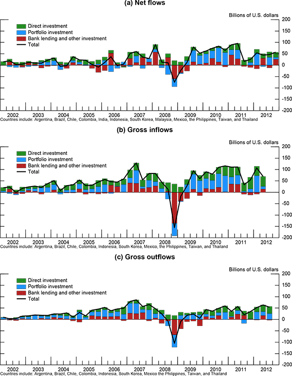
Source: Balance of payments (BOP) data collected from national sources. Gross inflows are BOP liabilities, and consist of the non-residents' purchases of domestic assets net of sales. Gross outflows are BOP assets, and consist of the residents' purchases of foreign assets net of sales. Net inflows represent the difference between gross inflows and outflows. Panels (b) and (c) do not include India and Malaysia, for which some gross inflow components are not available. Note that a gross outflow is reported in panel (c) with the plus sign, in contrast with the usual BOP practice.

Figure 2: Cumulative Net Inflows to EMEs

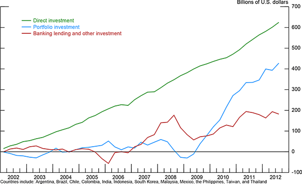
Source: BOP data collected from national sources.

Figure 3: Real Effective Exchange Rates in EMEs

Source: Federal Reserve Board.

Figure 4: Reserves Accumulation Since End-2005

Source: Haver Analytics.

Figure 5: Real Policy Rates and Output Gaps: Aggregate of Selected EMEs

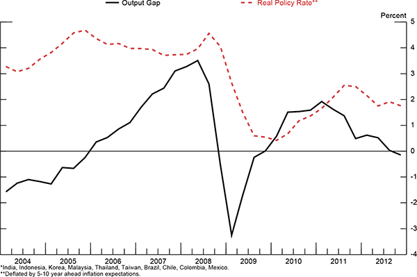
Source: Federal Reserve Board staff calculations. The output gap is expressed as the percent deviation of real GDP from its potential level, where the potential level is the Hodrick-Prescott trend of log-real GDP over 1994:Q4-2012:Q2. The aggregate is weighted in proportion to each country's share in U.S. exports.

Figure 6: Some Key Determinants of Net Inflows to EMEs

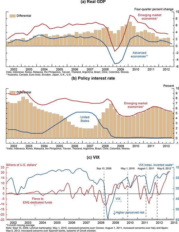
Source: Haver Analytics for quarterly real GDP (expressed as the 4-quarter percent change) and the nominal policy interest rates; Emerging Portfolio Fund Research for flows to EME-dedicated funds; Bloomberg for VIX.

Figure 7: Number of Capital Control Measures Introduced in EMEs Since 2009

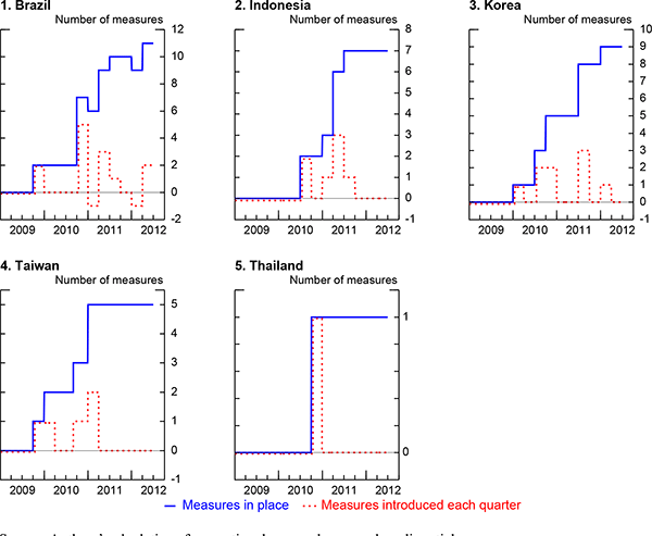
Source: Authors' calculations from national press releases and media articles.

Figure 8: Fitted Values vs. Counterfactuals for Total Net Inflows

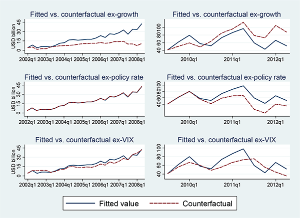
Note: The fitted values and counterfactuals are based on the model with country fixed effects, estimated separately for the periods 2002:Q1-2008:Q2 and 2009:Q2 to 2012:Q2. The counterfactuals are the fitted values obtained under the assumption that a particular determinant was equal to its initial value for each interval.

Figure 9: Fitted Values vs. Counterfactuals for Portfolio Net Inflows

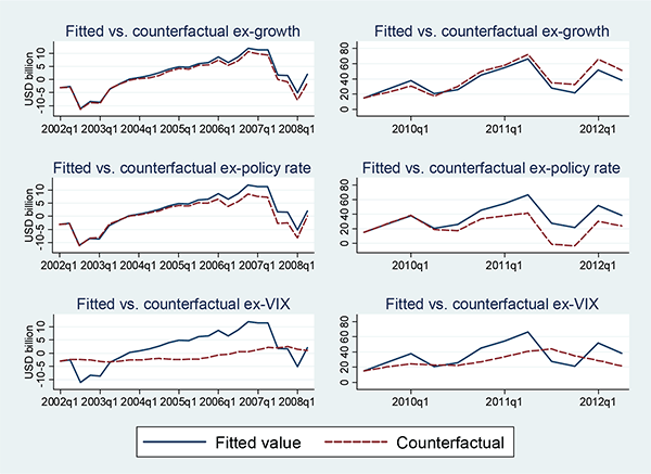
Note: The fitted values and counterfactuals are based on the model with country fixed effects, estimated separately for the periods 2002:Q1-2008:Q2 and 2009:Q2 to 2012:Q2. The counterfactuals are the fitted values obtained under the assumption that a particular determinant was equal to its initial value for each interval.

Figure 10: Shifting Behavior of Net Inflows Since 2008-09

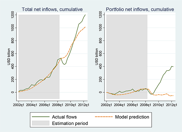
Note: The model predictions are based on results from the model with fixed effects estimated over the period 2002:Q1 to 2008:Q2.

Figure 11: Indicator Variables for LSAP Events

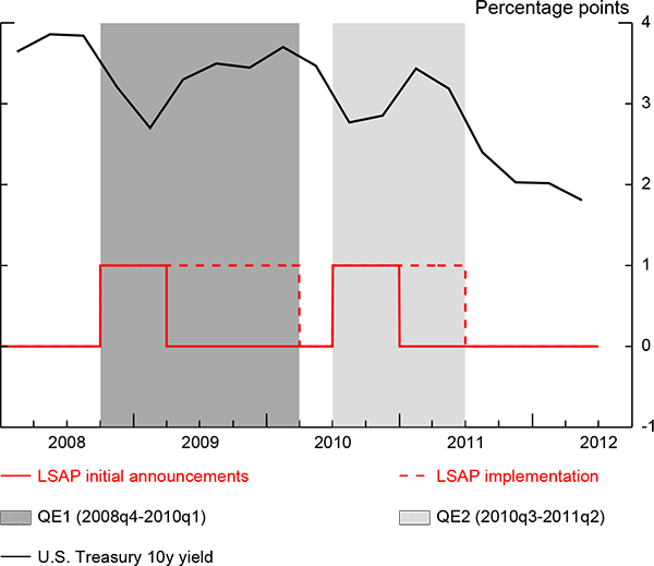
Note: The "initial announcements" variable equals 1 in 2008:Q4 and 2009:Q1 for QE1 and in 2010:Q3 and 2010:Q4 for QE2, when the corresponding programs were announced or extended. The "implementation" variable equals 1 for 2008:Q4-2010:Q1 and 2010:Q3-2011:Q2.

Figure 12: LSAP Purchases

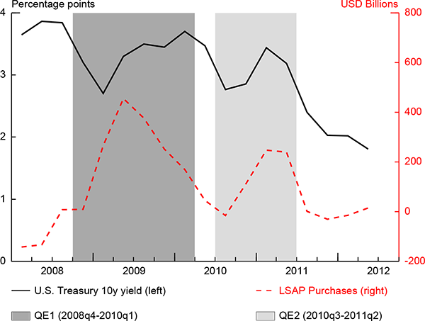
Source: Bloomberg (for the Treasury bond yield) and the Federal Reserve (for asset purchases). The net asset purchases are obtained as the change in the end-of-quarter total holdings of agency debt securities, mortgage-backed securities, and U.S. Treasury securities by the Federal Reserve.

Table 1: Capital Control Measures Introduced in EMEs Since 2009

Country	Restrictions on portfolio flows: Tax on foreign investments	Restrictions on portfolio flows: Restrictions by asset type or maturity	Restrictions on banking flows: Tax on short-term external borrowing	Restrictions on banking flows: Quantitative limits on banks' FX exposure	Restrictions on banking flows: Required reserves on FX liabilities
Brazil	Oct, Nov 09R, Oct, Dec 10R, Jul, Dec 2011R		Mar-Apr- Jul-Aug 11 Mar- Jun-Dec 12		Jan, Jul 11, Dec 12
Indonesia		Mar, Jun 10, Apr 11		Jun, Dec 10	Dec 10R
South Korea	Nov 10R, Jan 12R	Jul 11	Apr 11	Nov 09D, Jan 10, Jun 10D, Jun 11D, Nov 12D
Taiwan		Nov 09R Nov 10R		Dec 10D	Jan, Dec 10R
Thailand	Oct 10R

Source: Authors' calculations from national press releases and media articles (also see Figure 7). "R" denotes measures that discriminate by residency and "D" denotes limits on banks' FX derivatives positions.

Table 2: Summary Statistics

Period/Variable	Obs.	Mean %	Std. Dev. %-points	Min %	Max %
Pre-crisis period (2002q1-2008q2): tot_ngdp	312	0.55	5.73	-32.81	18.50
Pre-crisis period (2002q1-2008q2): port_ngdp	312	-0.33	4.30	-17.08	16.49
Pre-crisis period (2002q1-2008q2): growth_diff_ae	312	2.95	2.76	-16.12	9.11
Pre-crisis period (2002q1-2008q2): growth_eme	312	5.19	2.92	-15.22	11.83
Pre-crisis period (2002q1-2008q2): growth_ae	312	2.24	0.63	0.89	3.26
Pre-crisis period (2002q1-2008q2): policy_rate_diff_us	312	2.94	4.60	-4.60	25.18
Pre-crisis period (2002q1-2008q2): policy_rate_eme	312	5.82	4.39	0.49	26.44
Pre-crisis period (2002q1-2008q2): policy_rate_us	312	2.87	1.61	1.00	5.26
Pre-crisis period (2002q1-2008q2): treas_10yr_us	312	4.37	0.41	3.60	5.08
Pre-crisis period (2002q1-2008q2): vix	312	18.39	6.33	11.03	35.07
Pre-crisis period (2002q1-2008q2): interv_2y_ngdp	234	2.14	2.49	-1.75	12.11
Crisis period (2008q3-2009q2): tot_ngdp	48	-2.47	9.56	-38.96	17.21
Crisis period (2008q3-2009q2): port_ngdp	48	-1.97	6.01	-27.74	7.74
Crisis period (2008q3-2009q2): growth_diff_ae	48	3.62	3.88	-4.45	10.78
Crisis period (2008q3-2009q2): growth_eme	48	0.25	4.62	-9.59	8.09
Crisis period (2008q3-2009q2): growth_ae	48	-3.37	1.93	-5.14	-0.39
Crisis period (2008q3-2009q2): policy_rate_diff_us	48	4.58	3.41	-1.35	13.22
Crisis period (2008q3-2009q2): policy_rate_eme	48	5.30	3.49	0.53	13.75
Crisis period (2008q3-2009q2): policy_rate_us	48	0.71	0.74	0.18	1.96
Crisis period (2008q3-2009q2): treas_10yr_us	48	3.26	0.41	2.70	3.84
Crisis period (2008q3-2009q2): vix	48	40.41	12.78	25.07	58.54
Crisis period (2008q3-2009q2): interv_2y_ngdp	36	2.22	3.23	-5.07	9.93
Post-crisis period (2009q3-2012q2): tot_ngdp	144	1.87	4.74	-12.37	23.43
Post-crisis period (2009q3-2012q2): port_ngdp	144	1.07	4.43	-12.75	22.03
Post-crisis period (2009q3-2012q2): growth_diff_ae	144	3.90	2.92	-10.04	12.69
Post-crisis period (2009q3-2012q2): growth_eme	144	5.09	3.38	-8.79	13.65
Post-crisis period (2009q3-2012q2): growth_ae	144	1.20	1.81	-3.87	3.06
Post-crisis period (2009q3-2012q2): policy_rate_diff_us	144	3.78	2.68	0.11	12.19
Post-crisis period (2009q3-2012q2): policy_rate_eme	144	3.91	2.67	0.27	12.28
Post-crisis period (2009q3-2012q2): policy_rate_us	144	0.14	0.04	0.08	0.19
Post-crisis period (2009q3-2012q2): treas_10yr_us	144	2.89	0.65	1.81	3.70
Post-crisis period (2009q3-2012q2): vix	144	22.80	4.37	17.48	30.58
Post-crisis period (2009q3-2012q2): interv_2y_ngdp	108	3.11	3.50	-3.75	11.94

Table 3: Determinants of Net Private Capital Inflows: Basic Results*

Dependent variable:	(1) Total net inflows/NGDP	(2) Total net inflows/NGDP	(3) Total net inflows/NGDP	(4) Total net inflows/NGDP	(5) Portfolio net inflows/NGDP	(6) Portfolio net inflows/NGDP	(7) Portfolio net inflows/NGDP	(8) Portfolio net inflows/NGDP
Interval:	2002q1-2008q2	2002q1-2008q2:	2009q3-2012q2:	2009q3-2012q2:	2002q1-2008q2:	2002q1-2008q2:	2009q3-2012q2:	2009q3-2012q2:
Model:	OLS	FE	OLS	FE	OLS	FE	OLS	FE
growth_diff_eme-ae	0.48*** (0.12)	0.43*** (0.13)	0.34*** (0.13)	0.53 (0.14)	0.17* (0.091)0.16***	0.045 (0.095)	0.060 (0.13)	0.19 (0.13)
policy_rate_diff_eme-us	0.22*** (0.073)	0.0047 (0.16)	0.63*** (0.14)	0.70* (0.38)	0.16*** (0.055)	-0.055 (0.11)	0.34** (0.14)	0.58 (0.35)
vix	-0.060 (0.051)	-0.036 (0.052)	-0.12 (0.084)	-0.12 (0.079)	-0.095** (0.038)	-0.075** (0.037)	-0.13 (0.083)	-0.13* (0.072)
Constant	-0.40 (1.09)	-2.59* (1.53)	0.93 (2.09)	-0.66 (2.28)	0.43 (0.83)	-0.45 (1.09)	2.42 (2.07)	2.19 (2.07)
Observation	312	312	144	144	312	312	144	144
R-squared	0.063	0.154	0.158	0.319	0.046	0.227	0.055	0.357
F-test 1	0.40	2.06			0.11	0.94
Prob > F	0.67	0.13			0.89	0.39
F-test 2			0.11	0.12			0.083	0.060
Prob > F			0.74	0.73			0.77	0.81

Standard errors in parentheses

*** p<0.01, ** p<0.05, * p<0.1

Note: F-test 1 refers to the joint null hypothesis that the coefficients on EME growth and AE growth, as well as on the EME policy rate and the U.S. policy rate are equal in magnitude but opposite in sign. Similarly, F-test 2 refers to the null hypothesis that the coefficients on EME growth and AE growth are equal but opposite in sign. For the post-crisis period, F-test 1 is not applicable, because the U.S. policy rate was zero, and hence the policy rate differential is driven entirely by changes in the EME policy rate. *Economies included are India, Indonesia, Malaysia, the Philippines, South Korea, Taiwan, and Thailand from emerging Asia, and Argentina, Brazil, Chile, Colombia, and Mexico from Latin America.

Table 4: Structural Break Tests for the Determinants of Net Inflows*

Dependent variable:	(1) Total net inflows/NGDP	(2) Total net inflows/NGDP	(4) Portfolio net inflows/NGDP	(5) Portfolio net inflows/NGDP
Interval:	2002q1-2012q2	2002q1-2012q2:	2002q1-2012q2:	2002q1-2012q2:
Model:	OLS	FE	OLS	FE
growth_diff_eme-ae	0.48*** (0.11)	0.43*** (0.12)	0.17* (0.092)	0.045 (0.094)
policy_rate_diff_eme-us	0.22*** (0.069)	0.0047 (0.15)	0.16*** (0.056)	-0.055 (0.11)
Vix	-0.060 (0.048)	-0.036 (0.048)	-0.095** (0.039)	-0.075** (0.037)
post-crisis * growth_diff_eme-ae	-0.14 (0.19)	0.095 (0.21)	-0.11 (0.15)	0.15 (0.16)
post-crisis * policy_rate_diff_eme-us	0.41** (0.18)	0.69 (0.49)	0.17 (0.15)	0.63* (0.37)
post-crisis * Vix	-0.061 (0.11)	-0.086 (0.11)	-0.030 (0.090)	-0.053 (0.082)
post-crisis	1.33 (2.69)	-2.75 (4.21)	2.00 (2.19)	-2.45 (3.19)
Constant	-0.40 (1.02)	1.42 (2.32)	0.43 (0.83)	2.81 (1.76)
Observation	456	456	456	456
R-squared	0.097	0.204	0.070	0.286

Standard errors in parentheses, *** p<0.01, ** p<0.05, * p<0.1

Note: post-crisis is an indicator variable that equals 1 for the period 2009:Q3-2012:Q2. The fixed effects, when included (columns 2 and 4), are allowed to vary across the pre-crisis and post-crisis periods. *Economies included are the same as in table 3.

Table 5: The Effect of Capital Controls on Net Inflows*

Dependent variable:	(1) Total net inflows/NGDP	(2) Total net inflows/NGDP	(3) Total net inflows/NGDP	(4) Total net inflows/NGDP	(5) Portfolio net inflows/NGDP	(6) Portfolio net inflows/NGDP	(7) Portfolio net inflows/NGDP	(8) Portfolio net inflows/NGDP
Interval:	2009q3-2012q2	2009q3-2012q2	2009q3-2012q2	2009q3-2012q2	2009q3-2012q2	2009q3-2012q2	2009q3-2012q2	2009q3-2012q2
Model:	OLS	FE	OLS	FE	OLS	FE	OLS	FE
growth_diff_eme-ae	0.23* (0.13)	0.43*** (.15)	0.30** (0.13)	0.50 (0.14)	-0.029 (0.13)	0.090 (0.13)	0.036 (0.13)	0.18 (0.13)
policy_rate_diff_eme-us	0.84*** (0.14)	0.84** (0.39)	0.83*** (0.15)	0.90** (0.40)	0.51*** (0.15)	0.72** (0.35)	0.48*** (0.15)	0.82* (0.36)
Vix	-0.13 (0.080)	-0.13* (0.078)	-0.12 (0.082)	-0.12 (0.079)	-0.13 (0.081)	-0.13* (0.070)	-0.12 (0.083)	-0.13* (0.071)
capital_controls_in_place	-0.54*** (0.15)	-0.44** (0.21)			-0.44*** (0.15)	-0.45** (0.19)
new_capital_controls			-0.43 (0.50)	-0.37 (0.53)			0.057 (0.51)	-0.076 (0.48)
1_new_capital_controls			-0.43 (0.51)	-0.36 (0.55)			-0.77 (0.51)	-0.96* (0.50)
12_new_capital_controls			-0.97* (0.52)	-0.79 (0.56)			-0.98* (0.52)	-1.05** (0.50)
13_new_capital_controls			-1.26** (0.53)	-1.04* (0.55)			-0.59 (0.53)	-0.59 (0.49)
Constant	1.54 (2.01)	-0.00087 (2.27)	1.04 (2.04)	-0.51 (2.27)	2.93 (2.02)	2.86 (2.05)	2.37 (2.05)	2.14 (2.05)
Observations	144	144	144	144	144	144	144	144
R-squared	0.234	0.342	0.226	0.345	0.113	0.385	0.102	0.393

Standard errors in parentheses
*** p<0.01, ** p<0.05, * p<0.1

Note: capital_controls_in_place is the number of capital control measures introduced since 2009 that are in place in any given quarter. new_capital_controls is the number of new capital control measures introduced in a given quarter (l, l2, l3 indicate lagged values). *Economies included are the same as in table 3.

Table 6: The Effect of Foreign Exchange Intervention on Net Inflows*

Dependent variable:	(1) Total net inflows/NGDP	(2) Total net inflows/NGDP	(3) Portfolio net inflows/NGDP	(4) Portfolio net inflows/NGDP	(5) No. of capital controls in place
Interval:	2002q1-2008q2	2002q1-2008q2	2002q1-2008q2	2002q1-2008q2	2009q3-20012q2
Model:	OLS	FE	OLS	FE	FE
growth_diff_eme-ae	0.32* (0.17)	0.22 (0.21)	0.16 (0.11)	0.0044 (0.13)
policy_rate_diff_eme-us	0.11 (0.082)	0.062 (0.16)	0.11* (0.055)	0.053 (0.10)
Vix	-0.061 (0.051)	-0.043 (0.051)	-0.071** (0.034)	-0.053 (0.033)
fx_intervention	0.085 (0.15)	0.45** (0.18)	-0.13 (0.10)	0.20* (0.12)	0.20** (0.095)
trend					0.35*** (0.048)
Constant	0.94 (1.22)	-3.60** (1.82)	0.81 (0.82)	-3.89*** (1.17)	-71.3*** (9.79)
Observations	234	234	234	234	108
R-squared	0.024	0.127	0.056	0.220	0.731

Standard errors in parentheses
*** p<0.01, ** p<0.05, * p<0.1

Note: fx_intervention is the extent of net foreign exchange intervention, expressed in U.S. dollars, cumulated over the previous 8 quarters (i.e. lagged t-1 to t-9), expressed as a percent of contemporaneous quarterly nominal GDP expressed in the same units. Since flows on the left hand side are also normalized by the same nominal GDP, the coefficient on fx_intervention in columns (1)-(4) has the interpretation of the effect on capital flows in billions of dollars of a $1 billion net FX intervention over the previous two years. Data on intervention generously provided by Matt Malloy-see Malloy (2013) for a description. *Economies included are the same as in table 3.

Table 7: Behavior of Net Flows to EMEs During LSAP Events*

Dependent variable:	(1) Total net inflows/NGDP	(2) Total net inflows/NGDP	(3) Total net inflows/NGDP	(4) Total net inflows/NGDP	(5) Portfolio net inflows/NGDP	(6) Portfolio net inflows/NGDP	(7) Portfolio net inflows/NGDP	(8) Portfolio net inflows/NGDP
Model:	OLS	FE	OLS	FE	OLS	FE	OLS	FE
Interval:	2002q1-2012q2	2002q1-2012q2	2002q1-2012q2	2002q1-2012q2	2002q1-2012q2	2002q1-2012q2	2002q1-2012q2	2002q1-2012q2
d_lsap_announcements	1.09 (1.12)	1.10 (1.07)			1.51* (0.87)	1.44* (0.82)
d_lsap_implementation			1.02 (0.88)	0.96 (0.85)			1.26* (0.69)	1.19* (0.65)
growth_diff_eme-ae	0.46*** (0.12)	0.47*** (0.13)	0.48*** (0.12)	0.48*** (0.13)	0.17* (0.094)	0.094 (0.097)	0.19** (0.094)	0.11 (0.098)
policy_rate_diff_eme-us	0.21*** (0.074)	0.12 (0.13)	0.22*** (0.074)	0.13 (0.13)	0.16*** (0.058)	0.045 (0.10)	0.17*** (0.058)	0.054 (0.10)
Vix	-0.073 (0.047)	-0.063 (0.046)	-0.063 (0.048)	-0.054 (0.046)	-0.093** (0.037)	-0.086** (0.035)	-0.080** (0.037)	-0.074** (0.036)
crisis * growth_diff_eme-ae	-0.46* (0.24)	-0.42* (0.23)	-0.49** (0.24)	-0.44* (0.23)	-0.36* (0.19)	-0.41** (0.18)	-0.39** (0.19)	-0.45** (0.18)
crisis * policy_rate_diff_eme-us	0.65** (0.26)	0.54** (0.26)	0.65** (0.26)	0.54** (0.26)	0.18 (0.21)	0.24 (0.20)	0.19 (0.21)	0.24 (0.20)
crisis * vix	-0.099* (0.051)	-0.093* (0.048)	-0.11** (0.052)	-0.100** (0.050)	-0.0014 (0.039)	-0.00069 (0.037)	-0.0089 (0.041)	-0.0076 (0.039)
post-crisis * growth_diff_eme-ae	-0.20 (0.20)	-0.12 (0.19)	-0.27 (0.21)	-0.18 (0.20)	-0.16 (0.15)	-0.060 (0.15)	-0.24 (0.16)	-0.14 (0.16)
post-crisis * policy_rate_diff_eme-us	0.65*** (0.20)	0.54** (0.21)	0.63*** (0.21)	0.52** (0.21)	0.38** (0.16)	0.26 (0.16)	0.36** (0.16)	0.24 (0.16)
post-crisis * vix	-0.0047 (0.053)	-0.0092 (0.052)	-0.010 (00.54)	-0.014 (0.052)	0.044 (0.041)	0.048 (0.040)	0.038 (0.042)	0.042 (0.040)
capital_controls_in_place	-0.52*** (0.20)	-0.38* (0.20)	-0.50** (0.20)	-0.36* (0.20)	-0.42*** (0.15)	-0.34** (0.16)	-0.40** (0.15)	-0.32** (0.16)
Constant	-0.068 (0.97)	-1.41 (1.28)	-0.32 (0.99)	-1.61 (1.29)	0.38 (0.76)	0.31 (0.99)	0.062 (0.77)	0.063 (0.99)
Observations	504	504	504	504	504	504	504	504
R-squared	0.139	0.234	0.140	0.234	0.095	0.216	0.096	0.216

Standard errors in parentheses, *** p<0.01, ** p<0.05, * p<0.1

Note: d_lsap_announcements is an indicator variable equal to 1 for the quarters in which the initial announcements of LSAPs, so-called "QE1" and "QE2," and the decisions to continue them were made (2008:Q4, 2009:Q1, 2010:Q3 and 2010:Q4). d_lsap_implementation is equal to 1 for the entire duration of the "QE1" and "QE2" programs (2008:Q4-2010:Q1 and 2010:Q3-2011:Q2). *Economies included are the same as in table 3.

Table 8: Effects of LSAP Purchases on Net Inflows Through the 10-Year U.S. Treasury Bond Yields*

Dependent variable:	(1) Total net inflows/NGDP	(2) Total net inflows/NGDP	(3) Total net inflows/NGDP	(4) Total net inflows/NGDP	(5) Portfolio net inflows/NGDP	(6) Portfolio net inflows/NGDP	(7) Portfolio net inflows/NGDP	(8) Portfolio net inflows/NGDP
Model:	OLS	FE	OLS	FE	OLS	FE	OLS	FE
Interval:	2002q1-2012q2	2002q1-2012q2	2002q1-2012q2	2002q1-2012q2	2002q1-2012q2	2002q1-2012q2	2002q1-2012q2	2002q1-2012q2
treas_10yr_us	-0.38 (0.57)	-0.53 (0.58)			-0.64 (0.44)	-0.86* (0.44)
treas_10yr_us * crisis	-0.057 (0.76)	0.011 (0.72)			-1.36** (0.59)	1.23** (0.55)
treas_10yr_us * post-crisis	0.63 (0.64)	0.62 (0.61)			0.66 (0.49)	0.70 (0.47)
lsap_purchases_effect			-1.63 (1.64)	-1.60 (1.57)			-2.35* (1.31)	-2.18* (1.24)
growth_diff_ae	0.47*** (0.12)	0.47*** (0.13)	0.26 (0.16)	0.24 (0.18)	0.16* (0.095)	0.062 (0.098)	0.22* (0.13)	0.12 (0.15)
Policy_rate_diff_us	0.21*** (0.075)	0.088 (0.14)	0.19** (0.080)	0.12 (0.14)	0.16*** (0.058)	-0.0097 (0.11)	0.18*** (0.064)	0.064 (0.11)
Vix	-0.066 (0.050)	-0.055 (0.049)	-0.036 (0.056)	-0.030 (0.054)	-0.11*** (0.039)	-0.099*** (0.037)	-0.092** (0.045)	-0.084* (0.043)
crisis * growth_diff	-0.49* (0.25)	-0.45* (0.25)	-0.28 (0.26)	-0.27 (0.25)	-0.25 (0.20)	-0.30 (0.19)	-0.42** (0.21)	-0.46** (0.20)
crisis * policy_diff	0.65** (0.27)	0.52** (0.26)	0.68** (0.26)	0.62** (0.26)	0.24 (0.21)	0.28 (0.20)	0.18 (0.21)	0.25 (0.20)
crisis * vix	-0.091 (0.071)	-0.091 (0.068)	-0.14** (0.060)	-0.14** (0.058)	0.095* (0.055)	0.082 (0.052)	-0.0071 (0.048)	-0.0082 (0.046)
post-crisis * growth_diff	-0.27 (0.22)	-0.17 (0.21)	-0.024 (0.23)	0.068 (0.23)	-0.20 (0.17)	-0.083 (0.16)	-0.23 (0.18)	-0.12 (0.18)
post-crisis * policy_diff	0.62** (0.21)	0.49** (0.22)	0.67*** (0.21)	0.57*** (0.21)	0.34** (0.16)	0.19 (0.17)	0.36** (0.16)	0.26 (0.17)
post-crisis * vix	-0.082 (0.095)	-0.091 (0.091)	-0.042 (0.058)	-0.050 (0.057)	-0.048 (0.074)	-0.058 (0.069)	0.053 (0.046)	0.052 (0.045)
no_meas_ext	-0.53*** (0.20)	-0.40* (0.21)	-0.51*** (0.20)	-0.34* (0.20)	-0.44*** (0.15)	-0.39** (0.16)	-0.40** (0.16)	-0.33** (0.16)
Constant	1.38 (2.78)	0.62 (2.80)	-0.040 (1.08)	-0.29 (2.16)	3.55 (2.16)	4.31** (2.14)	0.14 (0.86)	1.10 (1.72)
Observation	504	504	468	468	504	504	468	468
R-squared	0.140	0.235	0.127	0.233	0.106	0.227	0.093	0.216

Standard errors in parentheses, *** p<0.01, ** p<0.05, * p<0.1

Note: lsap_purchases_effect is the difference between the actual 10-year U.S. Treasury bond yield and an estimate of what the yield would have been without LSAPs. To construct this effect, we regress the 10-year U.S. Treasury bond yields on Fed purchases one quarter ahead over the period 2003:Q1-2012:Q2 and subtract from the fitted value the estimated constant and error terms. *Economies included are the same as in table 3.

Appendix: Capital Flows to Emerging Market Economies: A Brave New World?³⁸

This appendix explores the robustness of our main results from the paper to several alternative specifications. These include: (1) decomposing the growth and policy rate differentials into separate emerging market economy (EME) and advanced-economy (AE) variables; (2) adding smaller countries in emerging Asia and Latin America; (3) adding emerging Euro- pean countries as well and allowing for regional effects; (4) using Credit Suisse's global risk appetite index (GRAI) instead of VIX; and (5) focusing on gross inflows rather than net inflows.

A  Robustness

A.1  Decomposing Differentials into EME and Rest-of-the World Variables

To compare our results to others in the literature, we have separated the growth and policy rate differentials into their relative counterparts, namely the growth of EMEs separated from the growth of their AE trading partners, and the policy rates of EME separated from the U.S. policy rate. The results are presented in table A1. First, they show that the coefficients are generally of the expected sign, positive on EME growth and EME policy rates, and negative on AE growth and the U.S. policy rate. They are also roughly equal in magnitude in several cases, suggesting the differential models may be a fairly reasonable approximation to the more general models. Second, considering statistical significance, the EME variables and sometimes also the AE/U.S. variables are significance for total inflows (columns 1-4). For portfolio inflows, the significance of EME variables declines, and the AE variables are no longer significant (columns 5-8). Note, though, that since the AE growth and the U.S. policy rate do not differ across the cross-sections in the panel, it is a taller order for them to come out statistically significant. Finally, of course, we cannot estimate the effect of the U.S. policy rate in the post-crisis period because of a lack of variation in this variable given the the zero lower bound; hence, in the post-crisis period, the policy rate differentials entirely reflect changes in the EME policy rates.³⁹

A.2  Sensitivity to Adding Other Countries From Asia and Latin America

Additional economies are included from emerging Asia (Hong Kong, Singapore, and China starting in 2010) and from Latin America (Costa Rica, Peru, Uruguay and Venezuela). Note that due to only partial availability of data for the whole sample period, including the unavailability of quarterly Chinese data before 2010, the sample becomes an unbalanced panel. Overall, our core results are fairly robust to adding these additional economies from emerging Asia and Latin America, although there are some important differences. In the results for 17 EMEs reported in table A2 (with all the additional countries from above added, except the international financial centers Hong Kong and Singapore), generally the growth and policy interest rate differentials still affect capital flows positively and global risk aversion negatively, as in the results reported in table 3 of the paper. However, one exception is that for pre-crisis total net inflows, the policy rate differential switches in sign and is not statistically significant. In addition, when the Asian financial centers Hong Kong and Singapore are added to the sample (see table A3), for the portfolio flows model, the effect of growth differentials switches sign to become negative for the post-crisis period and actually is statistically significance negative. This reinforces our argument made earlier that flows to these international financial sectors may not be determined by the same considerations as those for other EMEs.

A.3  Regional Effects and Adding Countries From Emerging Europe

One interesting question is whether the sensitivity of capital flows to their main drivers differs across regions. To address this question, we add countries from emerging Europe to the sample, in addition to those from Asia and Latin America reported above, excluding Hong Kong and Singapore. The following economies from emerging Europe are added to the sample: Croatia, Czech Republic, Hungary, Kazakhstan, Latvia, Poland, Romania, Russia and Ukraine, which takes the sample to 26 EMEs. We also add interaction terms for the growth and policy rate differentials as well as VIX with regional dummy variables for Latin America and emerging Europe to see if the effects of these variables differ across regions. With emerging Asia as the baseline, the coefficients on these interaction terms measure how different the effects are for Latin America and Eastern Europe, respectively, compared to Asia. The results for the Asia effects, reported in the top three rows of table A4, reinforce our core results from table 3 of the main paper that growth differentials, policy rate differentials, and risk aversion all matter. In particular, risk aversion is now statistically significant for emerging Asia for both sub-periods and both specifications. But differences across regions are clearly visible. In particular, policy rate differentials appeared to matter significantly less in Latin America than in Asia in the pre-crisis period. And, for total net inflows, risk aversion is also less important for Latin America for both periods. For emerging Europe, risk aversion also appears to be play a significantly smaller role than in Asia in driving total net inflows.

A.4  Alternative Measure of Global Risk Aversion

As an alternative to VIX, we use Credit Suisse's Global Risk Appetite Index (GRAI) as a measure of global appetite for risk. GRAI is obtained as the coefficient from regressing the stock returns from a number of AEs and EMEs (computed over six-month intervals) on stock price volatility of the preceding 18 months. A tighter link between past stock price volatility and future stock returns is assumed to signal greater willingness to take more risk and, thus an increase in the GRAI indicates an increase in global risk appetite. Indeed, the results in table A5 show that GRAI is positively related to the EME capital flows and is statistically significant in nearly the same specifications as in table 3 of the paper, while the results for other determinants are also preserved.

A.5  Gross vs. Net Capital Fl‡ows

We examine whether the results based on gross capital inflows to EMEs support our previous findings for net capital inflows. Due to the data limitations discussed earlier, when looking at gross inflows, we had to drop India and Malaysia from our sample of 12 core EMEs. The results for gross inflows, shown in table A6 of the appendix, are somewhat different from those on net inflows reported in table 3 of the paper. In particular, there is still some evidence of the importance of growth differentials for total gross capital inflows, but not as much for policy rate differentials. However, the evidence for the importance of risk aversion is much stronger than in table 3, reinforcing those results.

Finally, as shown in table A7, the original results on capital controls are preserved in the model with gross inflows. All else equal, the number of measures in place and the number of new measures still dampen gross inflows of capital, both for total inflows and for portfolio inflows. And, in the specifications with capital controls, the effects of growth differentials and policy rate differentials on gross inflows are qualitatively fairly similar to the effects on net inflows reported in Table 5, although not quite as strong. Overall, the magnitude of the effects are different but the main conclusions still go through with the models that utilize gross inflows.

Table A1: Determinants of Net Inflows Decomposed by EMEs and Advanced Economy Factors, 12 EMEs*

Dependent variable:	(1) Total net inflows/NGDP	(2) Total net inflows/NGDP	(3) Total net inflows/NGDP	(4) Total net inflows/NGDP	(5) Portfolio net inflows/NGDP	(6) Portfolio net inflows/NGDP	(7) Portfolio net inflows/NGDP	(8) Portfolio net inflows/NGDP
Interval:	2002q1-2008q2	2002q1-2008q2	2009q3-2012q2	2009q3-2012q2	2002q1-2008q2	2002q1-2008q2	2009q3-2012q2	2009q3-2012q2
Model:	OLS	FE	OLS	FE	OLS	FE	OLS	FE
growth_eme	0.49*** (0.12)	0.40*** (0.13)	0.34*** (0.13)	0.53*** (0.14)	0.17* (0.092)	0.028 (0.096)	0.061 (0.13)	0.19 (0.13)
growth_ae	-0.71 (0.63)	-0.76 (0.61)	-0.41* (0.24)	-0.60** (0.24)	0.048 (0.48)	0.12 (0.44)	-0.0014 (0.24)	-0.15 (0.22)
policy_rate_eme	0.20*** (0.076)	-0.21 (0.19)	0.64*** (0.14)	0.77* (0.40)	0.16*** (0.057)	-0.15 (0.14)	0.34** (0.14)	0.59 (0.36)
policy_rate_us	-0.38* (0.22)	-0.28 (0.22)			-0.19 (0.17)	-0.097 (0.16)
vix	-0.090 (0.063)	-0.086 (0.061)	-0.13 (0.086)	-0.13 (0.081)	-0.086* (0.048)	-0.084* (0.044)	-0.12 (0.085)	-0.12* (0.073)
Constant	1.19 (2.40)	0.37 (2.52)	1.00 (2.18)	-1.72 (4.63)	-0.15 (1.82)	0.049 (1.82)	2.18 (2.17)	-1.48 (4.21)
Observations	312	312	144	144	312	312	144	144
R-squared	0.066	0.165	0.161	0.322	0.047	0.232	0.056	0.359

Standard errors in parentheses
*** p<0.01, ** p<0.05, * p<0.1

* Economies included are those included in table 3 of the paper: India, Indonesia, Malaysia, the Philippines, South Korea, Taiwan, and Thailand from emerging Asia, and Argentina, Brazil, Chile, Colombia, and Mexico from Latin America.

Table A2: Determinants of Net Inflows, 17 EMEs From Emerging Asia and Latin America*

Dependent variable:	(1) Total net inflows/NGDP	(2) Total net inflows/NGDP	(3) Total net inflows/NGDP	(4) Total net inflows/NGDP	(5) Portfolio net inflows/NGDP	(6) Portfolio net inflows/NGDP	(7) Portfolio net inflows/NGDP	(8) Portfolio net inflows/NGDP
Interval:	2002q1-2008q2	2002q1-2008q2	2009q3-2012q2	2009q3-2012q2	2002q1-2008q2	2002q1-2008q2	2009q3-2012q2	2009q3-2012q2
Model:	OLS	FE	OLS	FE	OLS	FE	OLS	FE
growth_diff_eme-ae	0.23*** (0.079)	0.16* (0.083)	0.33*** (0.11)	0.31** (0.13)	0.061 (0.053)	0.0058 (0.057)	-0.023 (0.087)	0.11 (0.099)
policy_rate_diff_eme-us	-0.028 (0.064)	-0.049 (0.11)	0.24** (0.10)	0.45 (0.33)	0.088** (0.043)	-0.063 (0.078)	0.12 (0.082)	0.46* (0.25)
vix	-0.0082 (0.052)	-0.012 (0.048)	-0.094 (0.078)	-0.096 (0.072)	-0.074** (0.035)	-0.057* (0.033)	-0.082 (0.063)	-0.087 (0.055)
Constant	0.079 (1.08)	8.52*** (1.93)	1.86 (1.94)	-5.58 (5.20)	0.44 (0.72)	0.60 (1.33)	2.27 (1.58)	-4.26 (3.97)
Observations	372	372	202	202	372	372	202	202
R-squared	0.030	0.268	0.062	0.269	0.023	0.218	0.021	0.329

Standard errors in parentheses, *** p<0.01, ** p<0.05, * p<0.1.

*Economies included are those in table 3 of the paper plus China (with data starting in 2010:Q1), Costa Rica, Peru, Uruguay, and Venezuela. The international financial centers (Hong Kong and Singapore) are excluded.

Table A3: Determinants of Net Inflows, 19 EMEs From Emerging Asia and Latin America Including Financial Centers*

Dependent variable:	(1) Total net inflows/NGDP	(2) Total net inflows/NGDP	(3) Total net inflows/NGDP	(4) Total net inflows/NGDP	(5) Portfolio net inflows/NGDP	(6) Portfolio net inflows/NGDP	(7) Portfolio net inflows/NGDP	(8) Portfolio net inflows/NGDP
Interval:	2002q1-2008q2	2002q1-2008q2	2009q3-2012q2	2009q3-2012q2	2002q1-2008q2	2002q1-2008q2	2009q3-2012q2	2009q3-2012q2
Model:	OLS	FE	OLS	FE	OLS	FE	OLS	FE
growth_diff_eme-ae	0.23** (0.094)	0.15* (0.088)	0.21 (0.13)	0.31** (0.15)	0.022 (0.11)	-0.038 (0.11)	-0.21 (0.15)	-0.28* (0.17)
policy_rate_diff_eme-us	0.14* (0.076)	-0.055 (0.12)	0.27** (0.13)	0.48 (0.45)	0.31*** (0.089)	-0.0014 (0.15)	0.39*** (0.14)	0.21 (0.49)
vix	-0.019 (0.059)	0.0062 (0.049)	-0.13 (0.10)	-0.13 (0.092)	-0.20*** (0.069)	-0.15*** (0.059)	-0.076 (0.11)	-0.073 (0.10)
Constant	-1.59 (1.25)	8.26*** (2.10)	2.82 (2.52)	0.69 (2.84)	0.30 (1.47)	2.26 (2.53)	0.67 (2.73)	3.56 (3.11)
Observations	424	424	226	226	424	424	226	226
R-squared	0.017	0.400	0.030	0.276	0.043	0.382	0.060	0.288

Standard errors in parentheses, *** p<0.01, ** p<0.05, * p<0.1.

*Economies included are those in table A2 plus the international financial centers (Hong Kong and Singapore).

Table A4: Determinants of Net Inflows, 26 EMEs*

Dependent variable:	(1) Total net inflows/NGDP	(2) Total net inflows/NGDP	(3) Total net inflows/NGDP	(4) Total net inflows/NGDP	(5) Portfolio net inflows/NGDP	(6) Portfolio net inflows/NGDP	(7) Portfolio net inflows/NGDP	(8) Portfolio net inflows/NGDP
Interval:	2002q1-2008q2	2002q1-2008q2	2009q3-2012q2	2009q3-2012q2	2002q1-2008q2	2002q1-2008q2	2009q3-2012q2	2009q3-2012q2
Model:	OLS	FE	OLS	FE	OLS	FE	OLS	FE
growth_diff_eme-ae	0.20 (0.26)	0.17 (0.30)	0.46*** (0.17)	0.49** (0.22)	0.16 (0.16)	0.0036 (0.19)	-0.051 (0.14)	-0.080 (0.17)
policy_rate_diff_eme-us	0.44** (0.20)	0.80** (0.35)	0.41 (0.29)	-0.21 (0.80)	0.45*** (0.12)	0.41* (0.22)	0.30 (0.23)	-0.77 (0.64)
vix	-0.26*** (0.063)	-0.14* (0.075)	-0.30*** (0.083)	-0.27** (0.12)	-0.14*** (0.038)	-0.14*** (0.047)	-0.14** (0.067)	-0.22** (0.093)
growth_diff_eme-ae * d_latam	-0.15 (0.27)	-0.017 (0.32)	-0.40* (0.24)	-0.54* (0.30)	-0.16 (0.16)	0.0039 (0.20)	-0.027 (0.19)	0.19 (0.24)
policy_rate_diff_eme-us * d_latam	-0.63*** (0.22)	-1.00*** (0.38)	-0.43 (0.31)	0.96 (0.90)	-0.38*** (0.13)	-0.55** (0.24)	-0.24 (0.25)	1.56* (0.72)
vix * d_latam	0.14** (0.066)	0.23** (0.11)	0.24*** (0.077)	0.34** (0.16)	-0.0081 (0.039)	0.15** (0.069)	0.028 (0.062)	0.25* (0.13)
growth_diff_eme-ae * d_emeurope	0.039 (0.29)	-0.023 (0.36)	-0.70*** (0.21)	-0.65** (0.27)	-0.44** (0.17)	0.090 (0.23)	-0.043 (0.17)	0.036 (0.22)
policy_rate_diff_eme-us * d_emeurope	-0.71*** (0.23)	-1.07*** (0.39)	-0.54 (0.33)	-0.26 (1.05)	-0.35** (0.14)	-0.20 (0.24)	-0.50* (0.27)	0.32 (0.84)
vix * d_emeurope	0.40*** (0.069)	0.029 (0.10)	0.23*** (0.073)	0.047 (0.16)	0.088** (0.042)	0.017 (0.064)	0.090 (0.059)	0.081 (0.13)
Constant	4.09*** (0.98)	8.23** (3.54)	4.50** (1.75)	-13.9** (6.65)	1.37** (0.59)	-1.36 (2.22)	3.34** (1.41)	-11.8** (5.32)
Observations	593	593	310	310	593	593	310	310
R-squared	0.180	0.398	0.082	0.296	0.075	0.251	0.030	0.271

Standard errors in parentheses, *** p<0.01, ** p<0.05, * p<0.1.

*Economies included are those in table A2 plus Croatia, Czech Republic, Hungary, Kazakhstan, Latvia, Poland, Romania, Russia, and Ukraine.

Table A5: Determinants of Net Inflows With GRAI as Risk Variable, 12 EMEs*

Dependent variable:	(1) Total net inflows/NGDP	(2) Total net inflows/NGDP	(3) Total net inflows/NGDP	(4) Total net inflows/NGDP	(5) Portfolio net inflows/NGDP	(6) Portfolio net inflows/NGDP	(7) Portfolio net inflows/NGDP	(8) Portfolio net inflows/NGDP
Interval:	2002q1-2008q2	2002q1-2008q2	2009q3-2012q2	2009q3-2012q2	2002q1-2008q2	2002q1-2008q2	2009q3-2012q2	2009q3-2012q2
Model:	OLS	FE	OLS	FE	OLS	FE	OLS	FE
growth_diff_eme-ae	0.49*** (0.12)	0.43*** (0.13)	0.30** (0.13)	0.49*** (0.14)	0.19** (0.091)	0.054 (0.095)	0.032 (0.13)	0.16 (0.13)
policy_rate_diff_eme-us	0.21*** (0.073)	-0.010 (0.15)	0.66*** (0.14)	0.92** (0.42)	0.16*** (0.055)	-0.080 (0.11)	0.35** (0.14)	0.76** (0.38)
grai	0.12 (0.12)	0.071 (0.12)	0.25 (0.16)	0.25 (0.16)	0.21** (0.094)	0.16* (0.088)	0.17 (0.16)	0.21 (0.15)
Constant	-1.67*** (0.59)	-3.39*** (1.15)	-1.77** (0.86)	-3.34** (1.42)	-1.61*** (0.45)	-2.09** (0.83)	-0.38 (0.86)	-0.63 (1.30)
Observations	312	312	144	144	312	312	144	144
R-squared	0.061	0.153	0.161	0.319	0.042	0.255	0.047	0.351

Standard errors in parentheses, *** p<0.01, ** p<0.05, * p<0.1

*Economies included are those in table 3 of the paper.

Table A6: Determinants of Gross Inflows, 10 EMEs*

Dependent variable:	(1) Total gross inflows/NGDP	(2) Total gross inflows/NGDP	(3) Total gross inflows/NGDP	(4) Total gross inflows/NGDP	(5) Portfolio gross inflows/NGDP	(6) Portfolio gross inflows/NGDP	(7) Portfolio gross inflows/NGDP	(8) Portfolio gross inflows/NGDP
Interval:	2002q1-2008q2	2002q1-2008q2	2009q3-2012q2	2009q3-2012q2	2002q1-2008q2	2002q1-2008q2	2009q3-2012q2	2009q3-2012q2
Model:	OLS	FE	OLS	FE	OLS	FE	OLS	FE
growth_diff_eme-ae	0.069 (0.12)	0.11 (0.12)	0.19 (0.15)	0.34** (0.14)	-0.031 (0.082)	-0.048 (0.080)	0.094 (0.093)	0.21** (0.096)
policy_rate_diff_eme-us	-0.17** (0.069)	-0.22 (0.15)	0.15 (0.15)	-0.47 (0.41)	-0.073 (0.047)	-0.13 (0.094)	0.064 (0.095)	-0.025 (0.29)
vix	-0.18*** (0.051)	-0.17*** (0.050)	-0.25** (0.097)	-0.24*** (0.081)	0.10*** (0.035)	-0.097*** (0.032)	-0.15** (0.060)	-0.14** (0.057)
Constant	7.88*** (1.09)	9.52*** (2.31)	9.63*** (2.39)	6.22*** (2.27)	3.51*** (0.74)	4.56*** (1.49)	5.08*** (1.49)	2.72* (1.61)
Observations	260	260	120	120	260	260	120	120
R-squared	0.085	0.223	0.071	0.402	0.048	0.261	0.057	0.222

Standard errors in parentheses, *** p<0.01, ** p<0.05, * p<0.1

*Economies included are those in table 3 of the paper minus India and Malaysia, for which gross inflows are only partially available.

Table A7: The Effect of Capital Controls on Gross Inflows, 10 EMEs*

Dependent variable:	(1) Total gross inflows/NGDP	(2) Total gross inflows/NGDP	(3) Total gross inflows/NGDP	(4) Total gross inflows/NGDP	(5) Portfolio gross inflows/NGDP	(6) Portfolio gross inflows/NGDP	(7) Portfolio gross inflows/NGDP	(8) Portfolio gross inflows/NGDP
Interval:	2009q3-2012q2	2009q3-2012q2	2009q3-2012q2	2009q3-2012q2	2009q3-2012q2	2009q3-2012q2	2009q3-2012q2	2009q3-2012q2
Model:	OLS	FE	OLS	FE	OLS	FE	OLS	FE
growth_diff_eme-ae	0.088 (0.14)	0.30** (0.15)	0.19 (0.15)	0.32** (0.14)	0.037 (0.091)	0.087 (0.098)	0.080 (0.091)	0.18* (0.093)
policy_diff_eme-us	0.41** (0.16)	-0.39 (0.43)	0.40** (0.17)	-0.47 (0.44)	0.20** (0.10)	0.22 (0.29)	0.19* (0.10)	0.30 (0.30)
vix	-0.26*** (0.091)	-0.25*** (0.081)	-0.25*** (0.094)	-0.24*** (0.083)	-0.15** (0.058)	-0.15*** (0.055)	-0.14** (0.059)	-0.14** (0.055)
capital_controls_in_place	-0.61*** (0.16)	-0.15 (0.20)			-0.32*** (0.099)	-0.46*** (0.14)
new_capital_controls			-0.66 (0.53)	0.063 (0.51)			0.25 (0.33)	0.038 (0.34)
1_new_capital_controls			-0.69 (0.54)	0.23 (0.53)			-0.51 (0.34)	-0.77** (0.35)
12_new_capital_controls			-0.93* (0.55)	0.029 (0.54)			-0.87** (0.34)	-1.05*** (0.36)
13_new_capital_controls			-1.19** (0.55)	-0.34 (0.53)			-0.66* (0.35)	-0.77** (0.35)
Constant	10.4*** (2.26)	6.48*** (2.30)	9.71*** (2.32)	6.26*** (2.32)	5.48*** (1.44)	3.54** (1.55)	4.96*** (1.45)	2.73* (1.55)
Observations	120	120	120	120	120	120	120	120
R-squared	0.180	0.405	0.157	0.406	0.136	0.297	0.151	0.313

Standard errors in parentheses
*** p<0.01, ** p<0.05, * p<0.1

Note: capital_controls_in_place is the number of capital control measures introduced since 2009 that are in place in any given quarter. new_capital_controls is the number of new capital control measures introduced in a given quarter (l, l2, l3 indicate lagged values). *Economies included are those in table 3 of the paper minus India and Malaysia, for which gross inflows are only partially available.

Footnotes

*   Shaghil Ahmed ([email protected]) is an Assistant Director and Andrei Zlate ([email protected]) is an Economist in the International Finance Division of the Board of Governors of the Federal Reserve System, Washington, DC 20551. We would like to thank Joseph Byrne, Neil Ericsson, Steven Kamin, Patrice Robitaille, Frank Warnock, and participants at the fourth BIS-CCA research conference held at the Central Bank of Chile for their very helpful comments, as well as Andrew Brooks, Quoctrung Bui, and Zina Saijid for excellent research assistance. We are immensely grateful to Matt Malloy for providing his foreign exchange intervention data to us. The views in this paper are solely the responsibility of the authors and should not be interpreted as representing the views of the Board of Governors of the Federal Reserve System or any other person associated with the Federal Reserve System.  Return to text

1.   This paper, and the related literature we discuss, deals with private capital flows to EMEs. Even with strong private net capital inflows into EMEs in the pre- and post-global financial crisis periods, it is worth noting that total capital has flown "uphill" from the EMEs to the advanced economies because outflows through official channels (reserves accumulation) have been bigger. The role the influx of total capital into the United States played in lowering long-term U.S. yields in the runup to the global crisis has also been an important subject of discussion. See, for example, Bernanke (2005, 2007) and Bernanke et al. (2011).  Return to text

2.   There is an earlier literature focusing on heavy capital inflows to EMEs in the late 1980s and early 1990s. See, for example, Calvo, Leiderman, and Reinhart (1996), who found cyclical movements in world interest rates to be important. See also Taylor and Sarno (1997) who focused on the determinants of large portfolio flows from the United States to Latin America and Asia and found global and country-specific factors to be equally important.  Return to text

3.   See, also, IMF (2011b).  Return to text

4.   Among individual country studies, De Gregorio et al. (2000) focus on Chile over the period 1991-98; Cardenas and Barrera (1997) and Clements and Kamil (2009) focus on Colombia over the periods 1993-98 and 2007-08, respectively; Cardoso and Goldfajn (1998) focus on Brazil over the mid-1990s; and Coelho and Gallagher (2010) focus on Colombia and Thailand in the run-up to the 2008-09 crisis. Among panel studies, Montiel and Reinhart (1999) use an index measuring the incidence and intensity of capital account restrictions for 15 EMEs over the period 1990-96, and Binici, Hutchison, and Schindler (2009) use a measure of capital account restrictions from the IMFs' AREAER database for 74 countries. Miniane (2004) and Pasricha (2012) examine properties of capital control measures based on the IMF's AREAER classification of capital account restrictions. More broadly, Ostry et al. (2010) provide a survey on the effectiveness of capital controls prior to 2009. In contrast to the above studies, which do not find a persistent effect of controls on the volume of flows, a cross-country study, IMF (2007), suggests that episodes of capital inflow surges with tighter controls were associated with lower net private inflows. Also, Magu, Reinhart, and Rogoff (2011) find that certain country-specific characteristics need to exist for capital controls to be effective and, thus, not surprisingly, some capital controls were effective and some not. Return to text

5.   In addition, other studies, such as IMF (2007), have looked at the effect of foreign exchange intervention on the ability to actually moderate real exchange rate appreciations in the face of a persistent surge in capital flows, rather than at the direct effect on capital flows themselves. Return to text

6.   We will discuss later in the methodology section our rationale for focusing on these EME regions. Return to text

7.   "Banking and other flows'' include bank loans, trade credits, flows to deposit-taking corporations, and flows related to investments in financial derivatives. Return to text

8.   Gross banking flows are not available for India and Malaysia, and gross portfolio flows are discontinued for Malaysia in 2009:Q4. Return to text

9.   This changing view of capital controls has also been accompanied by a growing theoretical literature to more rigorously model the gains and costs of capital-account restrictions. Korinek (2011); Jeanne, Subramanian, and Williamson (2012)-in Chapter 2; and Jeanne (2012) review this literature. Using one such theoretical model calibrated to the Argentine economy, Bianchi (2011) computes the optimal tax on one-year foreign currency debt and finds that it could fluctuate between 0 and 22 percent, depending on conditions. Return to text

10.   This suggests that the relationship between the U.S. policy rate and capital flows to EMEs is capturing not just the effect of U.S. monetary policies, but of AE monetary policies more broadly. Return to text

11.   For the older literature on "sudden stops" and their effects on balance of payments and real exchange rates, see, for example, Calvo (1998) and Calvo et al. (2004). Also, Reinhart and Reinhart (2009) study capital flow "bonanzas," using a dataset covering 181 countries over the period 1980-2007.  Return to text

12.   IMF (2011a) also use gross inflows, applying the same model irrespective of the size of flows over the period 1990:Q1 to 2010:Q2, but ommitting two quarters during the crisis (2008:Q4 and 2009:Q1).  Return to text

13.   Papaioannou (2009) also finds institutional improvements to signficantly increase banking inflows.  Return to text

14.   To ensure that the quarterly volatility of nominal GDP does not affect our results, we have also normalized the net capital flows by the country-specific quadratic trend of nominal GDP computed over the sample period. The results are largely similar to the core results. Return to text

15.   The aggregate of advanced economies includes Australia, Canada, the euro area, Japan, Sweden, the United Kingdom, and the United States. Return to text

16.   For robustness, discussed in the Appendix, as an alternative to VIX we also use Credit Suisse's Global Risk Appetite Index (GRAI). Return to text

17.   These determinants can, of course, be correlated to some extent. For example, for the pre-crisis period, using a recursive VAR, Bruno and Shin (2013a) find that a higher Federal Funds rate was accompanied by an increase in risk-aversion, as measured by VIX.  Return to text

18.   Although this measure applies to both residents and non-residents, it may still affect capital inflows, since the short-term bills issued by Bank Indonesia (SBIs) were a favorite destination for carry trade investors. Return to text

19.   Notably, many of these measures have been characterized by EME authorities as macroprudential steps to promote financial stability rather than capital controls aiming to restrict the inflows. However, some of the measures have targeted only foreign investors, not domestic. In addition, measures that are not specifically aimed at foreign investors may still restrict the inflows indirectly, such as the restrictions applying to domestic borrowers rather than to foreign lenders, and therefore are included in our database. Return to text

20.   The measures introduced in the last month of every quarter were assigned to the following quarter. Return to text

21.   Finally, the IOF on foreign investment in equities and certain types of corporate bonds was eliminated in December 2011 (which is assigned to 2012:Q1), but subsequently the IOF on external borrowing by banks and firms was extended twice in 2012:Q2 to cover longer tenors. Return to text

22.   In Malloy (2013), the motivation is to explain what determines intervention, whereas in our paper we use the intervention data as an explanatory variable for capital flows. Return to text

23.   The net asset purchases are obtained as the change in the end-of-quarter total holdings of agency debt securities, mortgage-backed securities, and U.S. Treasury securities expressed in billions of U.S. dollars. For asset holdings, see http://www.federalreserve.gov/datadownload/, under " Factors Affecting Reserve Balances (H.4.1).''  Return to text

24.   We also attempted to estimate the same model over the crisis period, but it did not give significant results, perhaps due to the small sample of only four quarters and 12 EMEs. Using a broader sample consisting of both advanced economies and EMEs, Milesi-Ferretti and Tille (2011) identify the stylized facts and main drivers of the collapse of international capital flows during the global financial crisis. See, also, Ceterolli and Golberg (2010) for a discussion of the role of global banks in transmission of the 2007-2009 crisis to EMEs.  Return to text

25.   The dating of the crisis period here, from 2008:Q3 to 2009:Q2, is taken to be exogenously given. While this seems reasonable based on events affecting EMEs during the global financial crisis, it is possible that endogenizing the crisis period could result in these exact dates being off by a quarter or two. One way to empirically discover the exact structural break point is through Indicator Impulse Saturation analysis, a technique discussed in Hendry (1999) and Johansen and Nielsen (2009), inter alia. In future work, we intend to endogenously determine the break dates for the beginning and end of the crisis using such techniques. Return to text

26.   Note that even though the variables are statistically significant, the R-squared is moderate, indicated that some of the variation in capital inflows still remains unexplained by the variables included. One variable that is often suggested as an important determinant of EME capital flows is commodity prices (see, for example, Byrne and Fiess, 2011). But we have not included this variable here, as the effects of commodity prices on flows are likely to differ for commodity exporters and commodity importers, of which we have a mixture in our sample of EMEs. Return to text

27.   Obviously, the direction of causation can be an important issue in this argument. One counterargument is that capital flows may themselves magnifiy economic cycles in EMEs. To the extent that this holds and causation runs from capital flows to cyclical changes in EME output, the correlation between the two may still be a source of concern. In much of the recent work on the empirical determinants of capital flows, including this paper, it is assumed that causality runs primarily from growth prospects to capital flows. However, in some earlier empirical work, for example Cardarelli, Elekdag, and Kose (2009), which uses data on net inflows to 52 countries over the period 1987 to 2007, it is argued that although capital inflows tend to be associated with an accleration of GDP initially, subsequently growth can drop significantly. Kose et al (2009) and Jeanne, Subramanian, and Williamson (2012)-in Chapter 3-more broadly survey the empirical evidence on the growth benefits of capital account liberalization and do not find in the literature any robust benefits. Kose, Prasad, and Taylor (2011) argue that it has been difficult to empirically identify such benefits because the indirect benefits of financial integration may be more important than the traditional financing channels usually emphasized.  Return to text

28.   Pradhan et al. (2011) discuss how the properties of capital flows have changed between the pre- and post-crisis periods. Return to text

29.   Arias et al. (2012) also consider structural breaks between the pre- and post-crisis in the determinants of net private capital flows to EMEs, but using annual data that ends in 2010. Return to text

30.   Note that our measures of capital controls are indicator variables and do not account for the intensity of each control measure introduced. A useful extension would be to construct a more comprehensive measure of capital controls in which a judgment would be made on the intensity based on the specific details of each measure. Return to text

31.   Since the number of capital controls in place is a variable that has an upward trend over the post-crisis period, it is important to note that once a time-trend is included separately, this variable still has a statistically significant, negative effect on capital flows. Thus, the result is not spurious. Return to text

32.   Of course, capital controls are endogenous; in particular, it has been argued that such controls are more likely to be imposed at times of heavy capital inflows. However, this would bias against finding a negative effects of controls on flows, and thus does not detract from our results. Also, the endogeneity is partially addressed by the use of lagged values of capital control restrictions. But it could be argued that if news about imposition of controls is leaked in advance, investors may choose to bring in capital in advance of the imposition of controls, and subsequently flows might be seen to slow. To address such circumstances would require a fuller model in which capital controls were endogenously determined. Return to text

33.   Some country-specific case studies find singnificant changes in the composition of capital flows following the introduction of capital controls since the global financial crisis. See, for example, IMF (2011a) and, for the case of Brazil, Forbes et al. (2012). In addition, Gallagher (2011) also focuses on some of the more recent capital controls but considers their effects on interest rates, exchange rates and asset prices in Brazil, Korea, and Taiwan, rather than directly on capital inflows. Some have also argued that the recent capital controls imposed by countries lead to spillover effects in terms of increased flows to other countries. For example, Lambert, Ramos-Tallada, and Rebillard (2011), and Forbes et al. (2012), find that increases in Brazil's capital recent tax on foreign investment (the IOF tax) were associated with re-allocations of capital flows to other EMEs in Latin America.  Return to text

34.   A more satisfactory framework would be one that simultaneously models FX intervention at the same time as studying its effects on future flows, which we leave for future research. Return to text

35.   An alternative interpretation could be that a larger war chest of precautionary reserves in a country boosts investor confidence in that country. Return to text

36.   If we estimate LSAP effects without the crisis period observations, both with the variables used in table 7 as well as other variables related to LSAPs that are used later in table 8, the effects of capital flows from LSAPs are statistically insignificant, although still economically meaningful. Also, removing the crisis period observations results in a higher sensitivity of post-crisis flows to growth differentials and risk-aversion in the post-crisis period than implied by the results in table 7 (or table 8 shown later).  Return to text

37.   In the first-stage regression, the coefficient on the one-quarter ahead LSAP purchases is negative and statistically significant at the the 1% level, with about 10% of the variation in yields explained by future LSAPs. Return to text

38.  The views expressed here are solely the responsibility of the authors and should not be interpreted as representing the views of the Board of Governors of the Federal Reserve System or any other person associated with the Federal Reserve System. Return to text

39.  By and large, these results are consistent with the importance of the EME's own growth performance as well as of risk aversion and U.S. interest rates that previous studies, such as IMF (2011a), and Ghosh et al. (2012) found using sample periods that ended earlier and used much less of the post-crisis period than is included in our study. Return to text

This version is optimized for use by screen readers. Descriptions for all mathematical expressions are provided in LaTex format. A printable pdf version is available. Return to text

Home | Economic research and data | Publications and education resources
Accessibility | Contact us
Last update: August 1, 2014