
Board of Governors of the Federal Reserve System
International Finance Discussion Papers
Number 1087, August 2013 --- Screen Reader
Version*
Export Dynamics in Large Devaluations1
NOTE: International Finance Discussion Papers are preliminary materials circulated to stimulate discussion and critical comment. References in publications to International Finance Discussion Papers (other than an acknowledgment that the writer has had access to unpublished material) should be cleared with the author or authors. Recent IFDPs are available on the Web at http://www.federalreserve.gov/pubs/ifdp/. This paper can be downloaded without charge from the Social Science Research Network electronic library at http://www.ssrn.com/.
Abstract:
We study the source and consequences of sluggish export dynamics in emerging markets following large devaluations. We document two main features of exports that are puzzling for standard trade models. First, given the change in relative prices, exports tend to grow gradually following a devaluation. Second, high interest rates tend to suppress exports. To address these features of export dynamics, we embed a model of endogenous export participation due to sunk and per period export costs into an otherwise standard small open economy. In response to shocks to productivity, the interest rate, and the discount factor, we find the model can capture the salient features of export dynamics documented. At the aggregate level, the features giving rise to sluggish exports lead to more gradual net export reversals, sharper contractions and recoveries in output, and endogenous stagnation in labor productivity.
Keywords: Export dynamics, devaluation, net exports
JEL classification: E31, F12
1 Introduction
A widely held view in international economics is that it takes time for a change in the exchange rate to substantially change the pattern of international trade.2 Following large devaluations, this sluggishness is clearly evident for exports as the peak response occurs with a lag of three or four years. This sluggishness in exports is often attributed to the costs that producers face to adjust the markets or customers that they serve. The worsening financial conditions associated with devaluations may also weaken the export response by making it difficult for producers to finance export expansion.3 This gradual export expansion is thought to affect the dynamics of net exports and potentially output (Baldwin and Krugman, 1989). Here, we reconsider empirically and theoretically the source of sluggish export growth and its aggregate consequences. We document the salient micro and macroeconomic features of export dynamics in large devaluations. We then develop a small open economy model in which exports are determined in part by the entry decisions of non-exporters and the exit decisions of exporters. We show that the model can capture the observed sluggish growth of exports following a devaluation and that these export dynamics lead net exports to shift more gradually from deficit to surplus. We also find that these sluggish export dynamics lead to a deeper contraction and stronger recovery in output as well as a smaller depreciation. Additionally, the resources used to expand into new export markets leads measured labor productivity to stagnate.
We begin by characterizing the salient features of exports around large devaluations in 11 emerging markets. We focus on these periods of economic turmoil as these are large, easily identified events.4 First, we confirm that there is a gradual expansion of exports following a devaluation. The elasticity of exports to the real exchange rate is initially low and rises over time, peaking in the third year following the devaluation.5 Second, interest rates play a role in dampening export growth. Specifically, we find that in countries where interest rates rose more, as measured by the J.P. Morgan's EMBI spreads, the elasticity of exports to the real exchange rate is smaller. These two features hold when studying all exports as well as for exports to the US. Lastly, we examine the role of the extensive margin in the export dynamics with both product-level data for all the countries' export to the US and customs-level trade data for Argentina, Mexico, and Uruguay. Using these disaggregate data, we find that the extensive margin of trade (measured as number of products, destinations, and exporters) is important in this sluggishness and that the level of aggregation is important in measuring the role of the extensive margin in export growth.
These features of export dynamics pose a challenge for standard static trade models such as the Armington, Eaton-Kortum, or Melitz6 models. In these models, exports move proportionally to relative prices, implying a constant export elasticity, and there is no direct effect of interest rates on exports.7 We thus develop a small open economy model that can capture these gradual export dynamics and that has a role for the interest rate to affect exports. We embed a parsimonious model of producers starting and stopping to export into a small open economy that borrows to smooth consumption in response to aggregate shocks to the interest rate, productivity, and the discount factor (impatience). In our model, a country's exports depend on the stock of exporters actively selling overseas as well as the terms of trade. Over time, the stock of exporters can change as a result of costly investments by non-exporters to access foreign markets and by existing exporters to maintain their presence in foreign markets. Specifically, we follow the literature on export decisions (see Baldwin and Krugman (1989), Dixit (1989a b), Roberts and Tybout (1997), Das, Roberts and Tybout (2007), and Alessandria and Choi (2007)) and model the producer-level decision to export as involving both an up-front (or sunk) cost and an ongoing cost. We allow for idiosyncratic shocks to the costs of exporting. Thus, non-exporters will start exporting when the value of exporting exceeds the cost of starting to export. Similarly, exporters will continue to export as long as the value of exporting exceeds the cost of continuing to export. As long as the up-front cost is larger than the continuation cost, the stock of exporters is a durable asset that will adjust gradually to a shock. Profits from exporting are thus a return on the foregone resources to build up the stock of exporters. An increase in the interest rate will reduce the incentive to export by altering how the future benefits of exporting are discounted.
Our general equilibrium model allows us to identify the shocks that match the dynamics of output, interest rates, and real exchange rates observed in the data and evaluate the role of trade barriers on export, net export, and output dynamics. We find devaluations, and the associated economic crises, to be the result of a combination of increased international borrowing costs, less impatience,8 and a minor increase in observed productivity. In response to these shocks, the country would like to expand its exports by increasing the number of producers that export. However, the sunk aspect of export costs implies that the costs of expanding the stock of exporters are front-loaded while the benefits, measured as future export profits, are backloaded. Thus, to expand the stock of exporters requires the economy initially to devote substantial resources to invest in export capacity, which lowers current consumption relative to the future. The desire to smooth consumption thus puts a brake on the speed of export expansion. The intangible investment in export capacity tends to reduce a country's physical output initially and its ability to run a trade surplus therefore increasing its indebtedness. Given that the periods we study are characterized by both high interest rates and more patient consumers, the countries have little incentive to invest in expanding exports too quickly or strongly. Compared to a model without this dynamic exporting decision, this dampens export growth and leads to more gradual net export dynamics.
Our paper is related to a distinct and varied literature on international trade and macroeconomics. First, there is a literature that focuses on understanding why trade responds differently to changes in exchange rates or trade costs at different horizons. For instance, Baldwin and Krugman (1989), Dixit (1989a), Roberts and Tybout (1997), and Das, Roberts, and Tybout (2007) develop partial equilibrium models of sunk costs and real exchange rate fluctuations. Unlike these models, we develop a general equilibrium model that forces us to take a stand on the aggregate shocks, but allows us to evaluate the effect of these trade barriers on aggregate fluctuations in output and net exports. Ruhl (2003) and Alessandria and Choi (2011a,b) also develop general equilibrium models of sunk export costs, but they focus on the dynamics of trade growth in response to changes in trade barriers. In terms of business cycles, Alessandria and Choi (2007) develop a two-country GE model with sunk costs and find a minor impact on the dynamics of net exports in response to productivity shocks compared to a model without sunk costs. The larger effects here arise because we consider a different set of shocks (interest rates and impatience) and much larger shocks. Indeed, we find larger differences in how export costs affect aggregate fluctuations in response to interest rates shocks. Additionally, we explicitly consider the aggregate consequences in a particular calibration that generates export sluggishness, whereas the earlier Alessandria and Choi model did not generate much sluggishness. Drozd and Nosal (2012) and Engel and Wang (2011) also develop two-country GE models in which trade expands sluggishly over the business cycle. Unlike these models, we measure the sluggishness of exports in the data and evaluate the impact of the model to explain gross and net trade flows.
Our focus on emerging-market business cycles is related to papers by Neumeyer and Perri (2005), Uribe and Yue (2006) and Aguiar and Gopinath (2007). Unlike these papers, we explicitly model gross trade flows and consider their impact on output, net exports, and relative prices. A key feature of our model with relative prices fluctuations is that interest rates are now quite countercyclical as the increases in interest rates generate depreciations that reduce the incentive to produce and consume. Accounting for the contractionary effect of interest rates is a challenge in standard models, while here, due to the relative price changes they induce, the recessionary impact of interest rates is quite strong. Finally, Meza and Quintin (2007) and Kehoe and Ruhl (2008) have argued that an important puzzle to explain is the large decline in observed productivity in countries with large exchange rate movements. Here we find that overcoming the barriers to exporting lead measured labor productivity to lag TFP by as much as 8 percentage points while exports are expanding.
The paper is organized as follows. The next section documents the dynamics of exports, exchange rates, and interest rates in some emerging markets, using aggregate and disaggregate data. Section 3 develops our benchmark model and presents the model calibration. In Section 4 we examine the model's predictions for export dynamics. We conduct the sensitivity analysis in Section 5. Section 6 concludes.
2 Data
We begin by documenting some key relationships between exports, the real exchange rate, and interest rates in a sample of small open economies that experienced a large real exchange rate depreciation in the past two decades.9 Three salient features stand out. First, the elasticity of exports to the real exchange rate,10 measured as the change in exports relative to the change in the real exchange rate from prior to the devaluation, is quite low initially and rises over time. Second, high interest rates suppress exports as our export elasticity measure is more sluggish for countries that faced larger increases in international borrowing costs. Third, an important component of the gradual export response is a gradual rise in the extensive margin of trade, where the extensive margin is measured in various ways including by products, product-destinations, and firms. To establish these features, we move from the aggregate to disaggregate level.
2.1 Macro Data
Table 1 lists the 11 countries we consider along with the crisis dates. The sample is dictated by two considerations: The countries are small open economies that experienced a recent real exchange rate depreciation, and the data are available for at least 20 quarters after the event. The data appendix provides further details on the data sources and construction of all series.
Table 1
| Country | Crisis date |
|---|---|
| Argentina | December 2001 |
| Brazil | December 1998 |
| Colombia | June 1998 |
| Indonesia | July 1997 |
| Korea | October 1997 |
| Malaysia | July 1997 |
| Mexico | December 1994 |
| Russia | July 1998 |
| Thailand | June 1997 |
| Turkey | January 2001 |
| Uruguay | February 2002 |
Figure 1 summarizes some salient features in the events we study. The top panel shows the dynamics of the average exchange rate, interest rate, and exports in a 28-quarter window around the devaluations in these 11 emerging market economies. All variables are measured as the change from their levels on the eve of devaluation. The large devaluations are characterized by big real exchange rate depreciations, measured using the local CPI relative to the US CPI, and a spike in interest rates, measured as a JP Morgan EMBI spread. On average, the real exchange rate depreciates by about 40 to 50 log points initially and the interest rate spread rises about 1300 basis points.11 These increases exhibit some mean reversion, but remain elevated eight quarters after the devaluation. In contrast, the response of exports, measured in dollars, is muted. Over the first year, exports barely change from their pre-crisis level and then increase only gradually when the real exchange rate begins to appreciate.
The bottom panel shows that these export and relative price dynamics imply a relatively low elasticity of exports initially, which increases with time. We measure the elasticity of exports in quarter k as
| (1) | 
|
where ![]() is exports, P
is exports, P![]() is the US
import price deflator, and D is a measure of foreign real
expenditure12 (all measured as logs).13 This
measure isolates how the change in relative price induces
substitution towards the devaluing country's goods. We plot this
measure for overall exports and exports only to the US. The appeal
of using data on exports to the US is that the changes in the real
exchange rate and final expenditures are easier to compute and this
measure is consistent with our subsequent analysis of the extensive
margin of trade. The export elasticity is quite low initially,
averaging about 5 to 10 percent the first year, and then rises
steadily over the next three to four years to about 60 percent.
is the US
import price deflator, and D is a measure of foreign real
expenditure12 (all measured as logs).13 This
measure isolates how the change in relative price induces
substitution towards the devaluing country's goods. We plot this
measure for overall exports and exports only to the US. The appeal
of using data on exports to the US is that the changes in the real
exchange rate and final expenditures are easier to compute and this
measure is consistent with our subsequent analysis of the extensive
margin of trade. The export elasticity is quite low initially,
averaging about 5 to 10 percent the first year, and then rises
steadily over the next three to four years to about 60 percent.
The large spike in international borrowing costs suggests that the increase in the interest rate may contribute to the slow export growth. To explore this issue, we split our sample into two groups based on the cumulative increase in their interest rates 12 quarters following the crisis date.14 The high interest rate countries are Argentina, Malaysia, Indonesia, and Russia, while the low interest rate countries are Brazil, Colombia, Korea, Thailand, Turkey, and Uruguay.15
Figure 2 depicts the average interest rate and real exchange rate movements along with the mean export elasticity with respect to the real exchange rate to the US and to all countries for the two groups. These figures show that, on average, the high interest rate countries experienced a more than 2500 basis point increase in their interest rates, compared to the 500 basis point increase for the low interest rate countries. At the same time, the real exchange rate depreciation for the high interest rate countries is bigger and slightly less persistent. However, the export elasticity for the high interest rate countries is substantially below the level for the low interest rate countries at all horizons. For both groups, the export elasticity increases with time. The short-run elasticity is low, and the long-run elasticity is much higher.
2.2 Micro-Evidence on Export Dynamics
We now use disaggregated data to study some features of export dynamics following these devaluation episodes. First, we study the movements in the volume and variety of manufactured goods exported to the US. We focus on exports to the US because we have high-frequency disaggregated data for this destination for all countries. Also, the US is typically the largest trading partner for these countries, and thus exports to the US are likely to be somewhat representative of overall exports.
We find three main features: First, the volume of exports grows gradually. Second, the extensive margin grows gradually. Third, both the export elasticity and extensive margin elasticity for the high interest rate countries are lower than those for the low interest rate countries. Next, we analyze the extensive margin with customs-level trade data for Argentina, Mexico, and Uruguay to substantiate the role for the extensive margin. The customs-level trade data for Argentina are at the product and destination level. The customs-level trade data for the other two countries are at the firm, product, and destination level. Using this extensive data, we examine the importance of extensive margin in driving export dynamics for these three source countries. The customs-level data show that the US data tend to understate the role of the extensive margin in export growth.
2.2.1 Extensive Margin to US
To get a sense of what drives the gradual response in exports, we use more micro-oriented data to examine how the number of products and destinations changes following a devaluation. We undertake this analysis using highly disaggregated monthly US data on manufacturing imports (from the Census). An advantage of using these data is that we can also eliminate any concerns from the previous country-level analysis that the gradual increase in exports reflects a gradual increase in global economic activity or a change in the industry composition of exports. Specifically, to control for changes in the economic environment, we next consider how a devaluing country's exports to the US gain market share in US imports.16
We construct a trade-weighted measure of each country's import share,

where ![]() is US imports from country
is US imports from country ![]() of HS code
of HS code ![]() in period
in period ![]() and
and ![]() is share of imports for industry
j.17 To control for the rising share of
trade from China, we measure import shares relative to US imports
excluding China. The extensive margin is measured as a count of the
distinct number of HS-10 codes shipped to different US customs
districts. This is the finest level of disaggregation in the
publicly available trade data. To account for the growth in trade,
we also measure this as a share,
is share of imports for industry
j.17 To control for the rising share of
trade from China, we measure import shares relative to US imports
excluding China. The extensive margin is measured as a count of the
distinct number of HS-10 codes shipped to different US customs
districts. This is the finest level of disaggregation in the
publicly available trade data. To account for the growth in trade,
we also measure this as a share, ![]() of
the observed HS-10 destinations across all destinations. Since we
are focusing on a country's import share, we construct a measure of
its real exchange rate excluding the US and China.
of
the observed HS-10 destinations across all destinations. Since we
are focusing on a country's import share, we construct a measure of
its real exchange rate excluding the US and China.
Figures 3A and 3B summarize the average dynamics of each of these variables for our panel of 11 countries. The individual country dynamics are plotted in the appendix. To smooth out some of the variation in the data, we present statistics in six-month intervals.18 Figure 3A shows how our share measures vary over time. Figure 3B shows how our measures vary when we remove a log-linear trend rather than detrend with the share.
The first panel in each figure shows the dynamics of the trade-weighted real exchange rate for each country. In general, the real exchange rate depreciates about 30 to 40 percent over the first year. Over the subsequent three years the real exchange rate appreciates slightly; thus changes in relative prices are quite persistent. The second panel shows how our measure of the value of exports evolves. The third panel shows how the extensive margin evolves. The last panel shows how exports evolve with relative prices using a measure of the ratio of mean change in exports to the mean change in the real exchange rate. The elasticity of the export share is close to zero initially and rises to about 30 to 40 percent over 36 months. Depending on our de-trending it is one-third to twice as much over the first three years. In short, the evidence from the US is consistent with our finding using the aggregate data of a weak, gradual export response following a devaluation. The US data point to the extensive margin as being important in these export dynamics.
Lastly, we examine the dynamics of exports and extensive margin of exports from the high and low interest rate countries to the US respectively. Figure 4 shows that the high interest rate countries experience a bigger exchange rate devaluation in the first year. As in the aggregate data, the high interest rate countries experience slower export growth. The biggest gap in the export growth between the high and low interest rate countries is observed four years after the devaluation. In terms of the extensive margin, the difference between the high and low interest rate increase countries is smaller.19 The trade elasticities are also bigger for the low interest rate countries than for the high interest rate countries.
Our analysis based on counts provides some sense of the contribution of the extensive margin in export growth following devaluations. However, one might suspect that movements in our measure of the extensive margin might not contribute much to export growth if new exporters are much smaller than existing exporters. To adjust for this possibility, we now examine how important the extensive margin is in export growth. Following Eaton et al. (2007), we disaggregate the intensive margin from the exporters' margins of entry and exit as follows:
| (2) | 
|
where ![]() is the period of devaluation,
is the period of devaluation,
![]() denotes the total exports to
destination
denotes the total exports to
destination ![]() in year
in year ![]() , and
, and
![]() is exports by product or
firm
is exports by product or
firm ![]() to destination
to destination ![]() in period
in period
![]() . The term
. The term ![]() ,
,
![]() , and
, and ![]() represents the set of firms that exported in
represents the set of firms that exported in ![]() and
and ![]() , that exported in
, that exported in ![]() but not
but not ![]() , and that exported in
, and that exported in ![]() and not
and not ![]() , respectively. We refer to
these sets of firms as pairwise continuing, pairwise entering, and
pairwise exiting. The term is the intensive margin and captures the
change in imports from continuing exporters. The second and third
terms capture the lost volume from those that stopped exporting in
period
, respectively. We refer to
these sets of firms as pairwise continuing, pairwise entering, and
pairwise exiting. The term is the intensive margin and captures the
change in imports from continuing exporters. The second and third
terms capture the lost volume from those that stopped exporting in
period ![]() and the increased volume of exports from new
exporters.
and the increased volume of exports from new
exporters.
Because we are interested in the dynamics of intensive and extensive margins following devaluations, we decompose the cumulative growth of exports relative to the period of devaluations. Therefore, the intensive and extensive margins are the cumulative margins following devaluations.20
Figure 5 shows the share of export growth to the US accounted for by new products and new product-destinations rises steadily over the first twenty quarters after the devaluation. Initially, the extensive margin accounts for almost none of the export growth but by the end of the window it accounts for between 25 to 45 percent, with the larger share coming for the more disaggregate product-destinations pair measure. Thus, accounting for the relative size of entrants, exiters, and continuing products confirms an important role of the extensive margin for export growth.
2.2.2 Customs Data for Three Countries
We next examine the bias arising from using the 10-digit product level to the US rather than more disaggregate firm or destination data. We undertake this analysis using customs-level data for three countries. Figure 6 shows the share of exports to all destination due to the extensive margin for each of the three countries at different levels of aggregation. For each country, we decompose the extensive margin (using the Eaton method) at the most disaggregate product level and more disaggregate data on exports by destinations and firms.
For Argentina, since we lack firm-level data we go from 6-digit product to 10-digit product-destination level. From 12 quarters on, the more disaggregate data shows trade growth that is 3 to 4 times as large as the HS6 level. For Mexico, as we move from product to product-firm-destination level (HS-6) the contribution of the extensive margin more than triples. For Uruguay, moving from the HS-10 to HS-10-firm-destination level increases the contribution of the extensive margin by about 75 percent. Thus, the transaction-level data is consistent with the extensive margin being an important driver of the export response following devaluations. It also suggests that product level data may understate the movements of firms into new markets.
3 Model
We extend the basic model of a small open economy that borrows
and lends to smooth consumption to include endogenous entry and
exit from exporting. As is standard, the economy is subject to
exogenous shocks to the world interest rate, ![]() productivity,
productivity, ![]() and discount
factor,
and discount
factor, ![]() .21 These shocks lead to endogenous
fluctuations in the output, the real exchange rate, and trade.22
.21 These shocks lead to endogenous
fluctuations in the output, the real exchange rate, and trade.22
The economy produces two types of goods. A homogeneous domestic
nontradable, ![]() , is produced using labor,
, is produced using labor, ![]() There is an export sector with a unit mass of
imperfectly substitutable intermediate goods that can potentially
be exported. Each variety is produced with diminishing returns,23
There is an export sector with a unit mass of
imperfectly substitutable intermediate goods that can potentially
be exported. Each variety is produced with diminishing returns,23
![]() Each
producer has a different fixed cost of exporting so that in any
period only a subset, N, of the producers export.
Each
producer has a different fixed cost of exporting so that in any
period only a subset, N, of the producers export.
Specifically, we assume that cost of exporting depends on the
producer's export status in the previous period and an
idiosyncratic component. That is, non-exporters draw their cost
from a distribution
![]() and exporters draw
their cost from a different distribution
and exporters draw
their cost from a different distribution
![]() with
with
![]() These costs are valued in efficiency units of labor (i.e. scaled by
aggregate productivity) and cannot be recovered when a product is
no longer exported. When the cost of entering the export market
exceeds the cost of continuing in the marketplace, i.e.
These costs are valued in efficiency units of labor (i.e. scaled by
aggregate productivity) and cannot be recovered when a product is
no longer exported. When the cost of entering the export market
exceeds the cost of continuing in the marketplace, i.e.
![]() ,
exporting is a dynamic decision. We also assume that changing
export status takes one period so that the current measure of
exporters is predetermined.
,
exporting is a dynamic decision. We also assume that changing
export status takes one period so that the current measure of
exporters is predetermined.
Given these fixed export costs, it is well known that there will
be a threshold for non-exporters to start to export,
![]() and a threshold
for exporters to continue exporting,
and a threshold
for exporters to continue exporting,
![]() These thresholds
determine the fraction of non-exporters who start exporting,
These thresholds
determine the fraction of non-exporters who start exporting,
![]() and the
fraction of exporters who continue exporting,
and the
fraction of exporters who continue exporting,
![]() The law of
motion for the stock of exporters is
The law of
motion for the stock of exporters is
| (3) | 
|
Consumers consume a composite final good made by combining the
domestic good and foreign goods imported from abroad. Imports,
![]() are acquired using the revenue from
exporting and the net financing from international borrowing and
lending with one-period non-contingent bonds. The asset position is
denoted by
are acquired using the revenue from
exporting and the net financing from international borrowing and
lending with one-period non-contingent bonds. The asset position is
denoted by ![]() . The bonds are denominated in foreign
goods. To keep the model stationary, we allow for the country to
pay a premium above the world rate that is increasing in its debt
. The bonds are denominated in foreign
goods. To keep the model stationary, we allow for the country to
pay a premium above the world rate that is increasing in its debt
![]() .24The aggregate
state of the economy is thus
.24The aggregate
state of the economy is thus
![]()
We consider the problems of consumers, final good aggregators, and then exporters. We then sketch out the equilibrium conditions.
3.1 Consumer's Problem
Consumers start out the period with a stock of debt, ![]() . They also receive labor income,
. They also receive labor income, ![]() , and profits
from owning the exporters,
, and profits
from owning the exporters, ![]() . They are subject
to shocks to how they discount future utility (i.e.,
. They are subject
to shocks to how they discount future utility (i.e., ![]() changes over time). They choose how much to consume of
a final good and how much to borrow at rate
changes over time). They choose how much to consume of
a final good and how much to borrow at rate ![]() . The
Bellman equation is
. The
Bellman equation is

The first-order conditions are
| (4) | |||
| (5) |
3.2 Final Goods Market
The final consumption good is produced by a competitive final goods sector that combines domestic and foreign inputs and sells them at P. The aggregator's problem is
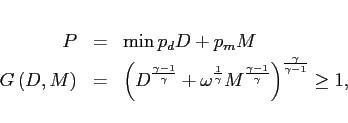
where ![]() is the Armington weight on the
imported good and
is the Armington weight on the
imported good and ![]() is the elasticity of
substitution between home and foreign goods. Given the Armington
structure, the price of the final good and allocations are
is the elasticity of
substitution between home and foreign goods. Given the Armington
structure, the price of the final good and allocations are
| (6) | 
|
||
| (7) | 
|
For simplicity we assume that domestic goods are produced in a perfectly competitive sector,
| (8) |  |
3.3 Export Sector
Potential producers in the export sector are characterized by
their predetermined export status, ![]() and current
idiosyncratic cost of exporting,
and current
idiosyncratic cost of exporting, ![]() .25
Fixed export costs are iid and the distribution depends on current
export status. Paying the cost to export allows the producer to
export in the following period. Exporters hire labor and face a
downward sloping demand curve:
.25
Fixed export costs are iid and the distribution depends on current
export status. Paying the cost to export allows the producer to
export in the following period. Exporters hire labor and face a
downward sloping demand curve:
![]() where
where
![]() is a demand
shifter that depends on the state of the economy. We first consider
the export decision, taking the pricing decision as given, and then
study the pricing decision.
is a demand
shifter that depends on the state of the economy. We first consider
the export decision, taking the pricing decision as given, and then
study the pricing decision.
The Bellman equation of a producer with export status
![]() and fixed export
cost
and fixed export
cost ![]() in aggregate state S is
in aggregate state S is

where
![]() denotes the profits from
exporting, and the cost of exporting depends on the cost draw
denotes the profits from
exporting, and the cost of exporting depends on the cost draw
![]() and aggregate productivity. Producers
discount the future with the stochastic discount factor
and aggregate productivity. Producers
discount the future with the stochastic discount factor
![]() This problem
implies that only producers with low fixed costs of exporting will
export. The export cost of the marginal exporter equals the
difference in the expected value of a potential exporter from being
an exporter or a non-exporter
This problem
implies that only producers with low fixed costs of exporting will
export. The export cost of the marginal exporter equals the
difference in the expected value of a potential exporter from being
an exporter or a non-exporter
| (9) | ![\begin{displaymath} \frac{w\kappa _{m}\left( S\right) }{z}=Eq^{\prime }\left[ V_{1}\left( S^{\prime }\right) -V_{0}\left( S^{\prime }\right) \right] =\frac{w\kappa ^{\ast }\left( S\right) }{z}. \end{displaymath}](img87.gif)
|
With iid entry shocks, the gain in export value is independent of
the current export status and therefore the threshold for starting
and continuing to export is identical (
![]() ).
Integrating over the distribution of entry costs, we can define the
expected values of starting as a non-exporter and an exporter as
).
Integrating over the distribution of entry costs, we can define the
expected values of starting as a non-exporter and an exporter as
![\begin{eqnarray*} EV_{0}\left( S\right) &=&-\frac{w}{z}\int_{0}^{\kappa ^{\ast }\left( S\right) }\kappa dF_{0}\left( \kappa \right) +q^{\prime }\left[ F_{0}\left( \kappa ^{\ast }\right) EV_{1}\left( S^{\prime }\right) +\left( 1-F_{0}\left( \kappa ^{\ast }\right) \right) EV_{0}\left( S^{\prime }\right) \right] , \ EV_{1}\left( S\right) &=&\pi -\frac{w}{z}\int_{0}^{\kappa ^{\ast }\left( S\right) }\kappa dF_{1}\left( \kappa \right) +q^{\prime }\left[ F_{1}\left( \kappa ^{\ast }\right) EV_{1}\left( S^{\prime }\right) +\left( 1-F_{1}\left( \kappa ^{\ast }\right) \right) EV_{0}\left( S^{\prime }\right) \right] . \end{eqnarray*}](img89.gif)
Defining the difference in the expected value of exporting as
.
yields a straightforward relationship between the current gain in the value of exporting and profits, export costs, and the future gain from exporting,
| (10) | 
|
Focusing on the steady state
![]() we get an
intuitive expression for the marginal exporter
we get an
intuitive expression for the marginal exporter
| (11) | 
|
The marginal entry cost is equal to the discounted expected profits
from exporting plus the savings in future costs of exporting. From
equation (11) we see that
an increase in the interest rate reduces the discounted expected
benefit from exporting and reduces the threshold for starting and
continuing to export. This implies that the entry into exporting is
reduced, and more exporters exit. When
![]() there
is no dynamic element to exporting.
there
is no dynamic element to exporting.
The pricing decision is straightforward. The firm faces a
downward sloping demand curve
![]() and cost of
labor of
and cost of
labor of ![]() . The final producer solves the following
problem:
. The final producer solves the following
problem:
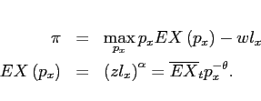
The optimal price is a markup over marginal cost
| (12) | 
|
||
| (13) | 
|
3.4 External Demand
To close the model, we assume that if ![]() exporters each charge
exporters each charge ![]() that aggregate export
revenue equals
that aggregate export
revenue equals
| (14) | 
|
where ![]() denotes the elasticity of
substitution between varieties and
denotes the elasticity of
substitution between varieties and ![]() the
elasticity of substitution between exports and domestic goods in
the ROW. In the appendix we show this equation can be derived from
the optimization problem of a representative agent in the ROW. This
implies that as the number of exporters expands they reduce the
sales of existing exporters. By varying
the
elasticity of substitution between exports and domestic goods in
the ROW. In the appendix we show this equation can be derived from
the optimization problem of a representative agent in the ROW. This
implies that as the number of exporters expands they reduce the
sales of existing exporters. By varying ![]() and
and
![]() we can change the relationship
between the export price, exporters, and aggregate exports. The
number of exporters, or the extensive margin of exports, affects
exports. For example, if
we can change the relationship
between the export price, exporters, and aggregate exports. The
number of exporters, or the extensive margin of exports, affects
exports. For example, if ![]() and
and ![]() then doubling the number of exporters increases
export revenues by 15 percent holding the export price constant. If
then doubling the number of exporters increases
export revenues by 15 percent holding the export price constant. If
![]() then doubling exporters
doubles exports.
then doubling exporters
doubles exports.
3.5 Equilibrium
We first describe the steady-state equilibrium. We will
calibrate and solve the model numerically in the subsequent
subsection. We assume consumers have GHH preferences
 , where
 ![]() is the risk aversion coefficient,
is the risk aversion coefficient,
![]() governs the labor supply elasticity,
and
governs the labor supply elasticity,
and ![]() is a scale parameter for the
aggregate labor supply. GHH preferences are widely used to study
the business cycles for small open economies as they eliminate the
wealth effect from the labor supply.
is a scale parameter for the
aggregate labor supply. GHH preferences are widely used to study
the business cycles for small open economies as they eliminate the
wealth effect from the labor supply.
An equilibrium is defined as a set of prices and allocations
![]() and firm
decisions
and firm
decisions
![]() such that (1) the
consumer's problem, final goods producer's problem, and exporter's
problem are solved, and (2) the markets clear. The equilibrium
conditions are given by equations (4)-(10), (12), and (13), as well
as the following market clearing condition.
such that (1) the
consumer's problem, final goods producer's problem, and exporter's
problem are solved, and (2) the markets clear. The equilibrium
conditions are given by equations (4)-(10), (12), and (13), as well
as the following market clearing condition.
| (15) | 
|
||
| (16) | 
|
||
| (17) | 
|
||
| (18) |
The first market clearing condition states that the market for each exported variety clears. The next equation is the market clearing condition for labor and requires the labor supplied to equal the resources used in production and in export costs. The last two conditions determine aggregate profits and the budget constraint. Given the curvature in the production of exported goods, it is useful to define the real exchange rate as the relative price of domestic consumed to imported goods or

We also define real output as

where the term
![]() adjusts for the
lack of markup on domestic goods, and the bars denote steady-state
prices. Finally, we measure net exports scaled by gross trade
flows:
adjusts for the
lack of markup on domestic goods, and the bars denote steady-state
prices. Finally, we measure net exports scaled by gross trade
flows:

3.6 Calibration
This subsection describes how we set the parameters in the model. Some parameters are based on standard values. Some parameters are chosen so that the steady-state equilibrium can match certain empirical moments. Finally, some other parameters are chosen to match the observed sluggish export dynamics.
First, we set the mean time discount factor ![]() , the risk aversion
, the risk aversion ![]() , and labor
supply parameter
, and labor
supply parameter ![]() to the standard values. The
elasticity of labor supply parameter
to the standard values. The
elasticity of labor supply parameter ![]() is taken
from Mendoza (1991). The weight on labor in the utility function,
is taken
from Mendoza (1991). The weight on labor in the utility function,
![]() is chosen so labor is one-third of
the time endowment. The interest elasticity parameter is chosen to
make the model stationary.
is chosen so labor is one-third of
the time endowment. The interest elasticity parameter is chosen to
make the model stationary.
Entry and continuation costs are assumed to be exponentially distributed,
![\begin{displaymath} F_{i}\left( k\right) =\left( \frac{k}{f_{i}v_{i}}\right) ^{\frac{1}{v_{i}-1}} \text{ for k}\in \left[ 0,f_{i}v_{i}\right] . \end{displaymath}](img141.gif)
The mass of exporters and persistence of exporting are primarily
determined by ![]() and
and ![]() while
the dynamic response of the extensive margin is primarily
determined by the dispersion of the costs. Note that as
while
the dynamic response of the extensive margin is primarily
determined by the dispersion of the costs. Note that as ![]() converges to 1, the distribution of costs becomes
degenerate at
converges to 1, the distribution of costs becomes
degenerate at ![]() . For simplicity, we set
. For simplicity, we set ![]() and then choose
and then choose ![]() to get the
response of the extensive margin in these devaluation episodes.
to get the
response of the extensive margin in these devaluation episodes.
Consistent with evidence in Das, Roberts, and Tybout (2007), we
assume that exporting is a very persistent activity. Empirical
evidence for the US is that about 10 to 12 percent of existing
exporters exit per year. Evidence for Colombia and Chile shows even
less exit from exporting. However, many of the exiting exporters
are relatively small, thus the share of trade accounted for exiting
exporters is less than the amount of exit. Since we have no
heterogeneity in production in the model, we target an exit rate of
1.5 percent per quarter so that
![]() which
then implies an entry rate,
which
then implies an entry rate,
![]() The ratio of entry to continuation cost
The ratio of entry to continuation cost
![]() determines the
exit rate, while
determines the
exit rate, while ![]() determines the fraction of
plants that export, which we set to 25 percent.
determines the fraction of
plants that export, which we set to 25 percent.
The elasticity of substitution, ![]() ,
curvature in production,
,
curvature in production, ![]() and elasticity of
substitution,
and elasticity of
substitution, ![]() will determine the dynamics of
the volume and variety of exports. Since part of our goal is to
evaluate the contribution of this sluggishness on aggregate
outcomes, we choose parameters so that the model can come close to
matching these export dynamics. We choose the curvature in the
production function,
will determine the dynamics of
the volume and variety of exports. Since part of our goal is to
evaluate the contribution of this sluggishness on aggregate
outcomes, we choose parameters so that the model can come close to
matching these export dynamics. We choose the curvature in the
production function, ![]() so that the export
price relative to the nontraded locally produced goods price (i.e.
P
so that the export
price relative to the nontraded locally produced goods price (i.e.
P
![]() ) moves about as much
as the ratio of the producer-price-based real exchange rate to the
consumer-price-based real exchange rate. We set
) moves about as much
as the ratio of the producer-price-based real exchange rate to the
consumer-price-based real exchange rate. We set ![]() so that exporter's price over average costs
(including fixed costs) is 12 percent. We set
so that exporter's price over average costs
(including fixed costs) is 12 percent. We set ![]() to come close to the average export elasticity
following these devaluations. This is well within the range of
typical values used in quantitative studies.
to come close to the average export elasticity
following these devaluations. This is well within the range of
typical values used in quantitative studies.
We assume the shocks each follow an AR(1) process of
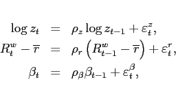
where
![]() We
then choose the sequence of shocks to
We
then choose the sequence of shocks to
![]() so
that the model can match the observed typical dynamics of
industrial production, the EMBI rate, and the real exchange rate in
our 11 devaluation episodes. Our focus will be on matching the
dynamics of these economies around devaluations, so we do not have
to take a stand on the variance of the shocks.26 Given that we
also target the extensive margin elasticity this essentially
involves trying to fit the model to four aggregate series.
so
that the model can match the observed typical dynamics of
industrial production, the EMBI rate, and the real exchange rate in
our 11 devaluation episodes. Our focus will be on matching the
dynamics of these economies around devaluations, so we do not have
to take a stand on the variance of the shocks.26 Given that we
also target the extensive margin elasticity this essentially
involves trying to fit the model to four aggregate series.
Given the preset parameters, we calibrate the remaining parameters to match the target statistics in the steady state as shown in Table 2.
Table 2a: Parameters (A. Predetermined)
| β | σ | η | ϒ |
| 0.99 | 2 | 1.5 | 1.3 |
Table 2b: Parameters (B. Calibrated Parameters)
| Parameters | Target |
|---|---|
| θ = 3 | markup =12% |
| debt/imports=10 | |
| ƒ0 | exporter ratio N=25% |
| ƒ1 | exit rate of exporter |
| v0 = v1 | avg. extensive margin elasticity:  |
| α | Ratio of PPI to CPI real exchange rate:  |
| ω | labor for exports = |
| λ | labor normalization (L=1/3) |
In particular, for the average debt level in the steady state,
we can set it so that
![]() (debt equal to b times
quarterly imports). With imports of 15 percent of GDP, this is
equivalent to a 37.5 percent Debt-to-GDP ratio.
(debt equal to b times
quarterly imports). With imports of 15 percent of GDP, this is
equivalent to a 37.5 percent Debt-to-GDP ratio.
To explore the importance of getting export dynamics right on
aggregate outcomes, we also consider a model with a static export
decision. In this model, which we call " no sunk," ![]() and entry is immediate. The fixed cost is set so
25 percent of producers export. Because the entry and continuation
costs are the same this implies there is substantial churning in
export status as only 25 percent of exporters continue each period
and that 25 percent of non-exporters start exporting each period.
The distribution of fixed costs is set to generate the same average
elasticity of exports to the real exchange rate given the shocks we
have backed out of our benchmark model.
and entry is immediate. The fixed cost is set so
25 percent of producers export. Because the entry and continuation
costs are the same this implies there is substantial churning in
export status as only 25 percent of exporters continue each period
and that 25 percent of non-exporters start exporting each period.
The distribution of fixed costs is set to generate the same average
elasticity of exports to the real exchange rate given the shocks we
have backed out of our benchmark model.
3.7 Disciplining the Export Elasticity
As discussed, the dynamics of the export elasticity are
primarily determined by three parameters,
![]() It is
straightforward to derive the relationship between these parameters
and the elasticity of exports to the real exchange rate from the
pricing and external demand equations, taking movements in wages
and productivity as given. To begin with, the change in exports per
firm depends on the change in exporters and the relative prices
It is
straightforward to derive the relationship between these parameters
and the elasticity of exports to the real exchange rate from the
pricing and external demand equations, taking movements in wages
and productivity as given. To begin with, the change in exports per
firm depends on the change in exporters and the relative prices
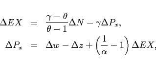
where the change in the export price just depends on the change in marginal cost, which depends in part on the change in exports because of the curvature in production. Substituting out the change in exports yields a formula for the change in the producer's prices

Note that changes in relative wages are quite large compared to
productivity and closely related to movements in the real excha![]() nge
rate so that
.
Obviously the first term just tells us that the price of exports
will move proportionally to the real exchange rate in the short-run
(
nge
rate so that
.
Obviously the first term just tells us that the price of exports
will move proportionally to the real exchange rate in the short-run
(![]() where the amount of the movement
is increasing in
where the amount of the movement
is increasing in ![]() and decreasing in
and decreasing in ![]() This is intuitive since a higher
This is intuitive since a higher ![]() means less curvature in production, while a higher
means less curvature in production, while a higher
![]() means a bigger export response. This
effect gets unwound a bit as more producers enter and they take
market share from the original exporters. Using this approximation
and then solving for aggregate nominal exports yields the export
elasticity:
means a bigger export response. This
effect gets unwound a bit as more producers enter and they take
market share from the original exporters. Using this approximation
and then solving for aggregate nominal exports yields the export
elasticity:
![\begin{displaymath} \frac{\Delta EXR}{\Delta rer}=\left[ \frac{\gamma -1}{\theta -1}+\frac{ \left( \gamma -1\right) \left( \frac{1}{\alpha }-1\right) \frac{\gamma -\theta }{\theta -1}}{1+\left( \frac{1}{\alpha }-1\right) \gamma }\right] \frac{\Delta N}{\Delta rer}-\frac{\gamma -1}{1+\left( \frac{1}{\alpha } -1\right) \gamma }. \end{displaymath}](img174.gif)
The first term shows the role of extensive margin. As the terms in
the bracket are positive, the final term determines the short-run
elasticity. It is decreasing in ![]() and
increasing in
and
increasing in ![]() Over time, the elasticity rises
as the extensive margin grows gradually, which shows up as the
first term increases.
Over time, the elasticity rises
as the extensive margin grows gradually, which shows up as the
first term increases.
When ![]() these terms reduce to
these terms reduce to
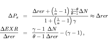
which tells us that ![]() pins down the
short-run elasticity while
pins down the
short-run elasticity while ![]() and the
and the
![]() determine the
long-run elasticity. Now recall that we can choose the distribution
of entry/continuation costs to get
determine the
long-run elasticity. Now recall that we can choose the distribution
of entry/continuation costs to get
![]() which then means
that given a
which then means
that given a ![]() there is a
there is a ![]() that generates an aggregate response similar to the
data. Given that the short-run response
that generates an aggregate response similar to the
data. Given that the short-run response ![]() is
close to 1.3 while in the long-run
is
close to 1.3 while in the long-run
![]() 0.6 while
0.6 while
![]() we
can solve for the elasticity as
we
can solve for the elasticity as

Thus, the model requires domestic varieties to be very poor
substitutes and hence exported varieties must be poor substitutes
to get the long-run elasticity given the changes in the extensive
margin. When ![]() the model has some more
flexibility to match the short- and long-run export elasticity.
the model has some more
flexibility to match the short- and long-run export elasticity.
4 Results
We summarize the properties of our model in Figures 7 and 8. The data on trade flows are based on bilateral flows with the US so that we can more precisely control for changes in external demand unrelated to movements in relative prices. Figure 7 plots the properties of our model, the data, and a model with no dynamic export decision (identified as no sunk cost) for a set of shocks that closely match the dynamics of output,27 interest rates, and the real exchange rate in our benchmark model. The top three panels plot our target series. Overall, the fit of the benchmark model is quite good. We can almost exactly match the output and interest rate series. The largest gap between the model and the data is in the real exchange rate over the first 5 quarters. In the data, the real exchange rate overshoots its longer-run level by about 10 percentage points, while the sunk cost model generates only a modest overshooting. The fourth panel depicts the elasticity of the extensive margin. We have chosen model parameters to match the average extensive margin elasticity from the data.
The fifth panel depicts the export elasticity, measured as the ratio of the change in exports to the change in the real exchange rate. Over the window we focus on, the average response in the model is quite close to the data (0.35 vs 0.37). Because of the dynamics of the extensive margin, the model generates some, but not all, of the gradual expansion of the export elasticity. In the model the export elasticity rises from 13 percent to 48 percent, while in the data the increase is from about 10 percent to 60 percent.
The final panel depicts a measure of the movements in net exports relative to the real exchange rate that controls for changes in expenditure growth across countries. Specifically, we measure

where D![]() is a measure of final expenditures
in the ROW and D
is a measure of final expenditures
in the ROW and D![]() is expenditures at home.28
Removing the difference in expenditure growth across countries
allows us to concentrate on how relative prices induce substitution
between domestic and foreign goods. In the data, net exports also
expand gradually relative to the real exchange rate with our net
export elasticity rising from about 50 percent to 150 percent over
12 quarters. The model with the dynamic export decision can capture
some, but not all, of this sluggishness. In a standard one-good SOE
model, the elasticity of net exports is, by definition, infinite.
is expenditures at home.28
Removing the difference in expenditure growth across countries
allows us to concentrate on how relative prices induce substitution
between domestic and foreign goods. In the data, net exports also
expand gradually relative to the real exchange rate with our net
export elasticity rising from about 50 percent to 150 percent over
12 quarters. The model with the dynamic export decision can capture
some, but not all, of this sluggishness. In a standard one-good SOE
model, the elasticity of net exports is, by definition, infinite.
The top panel of Figure 8 depicts the productivity, interest rate, and discount factor shocks required for the model to fit output, interest rates, and the real exchange rate. Along with a rise in interest rates, these episodes require a steady increase in productivity and patience of about 10 percentage points over the first six quarters that gradually mean revert. These productivity and discount factor dynamics are necessary to match the long-run increase in output with the depreciation 16 quarters on. The increase in productivity may be surprising given the decline in output and the well-known decline in measured labor productivity around devaluations (see Meza and Quintin, 2007, and Kehoe and Ruhl, 2008). However, in our model, measured labor productivity does not correspond to the shock we put through the model since the resources used to build up the stock of exporters do not increase current output. Measured labor productivity (Y/L) increases less on impact and is on average only 20 percent of the shock over the first year. Over time, labor productivity rises slowly but remains far below the TFP shock even four years on. The large gap between TFP and labor productivity arises because substantial resources are directed toward the intangible investment involved in preparing products for the export market. The mismeasurement of labor productivity owing to the resources devoted to building export capacity is potentially as important as other channels that we have abstracted from, such as variable capital utilization (Meza and Quintin), costly sector labor reallocation (Kehoe and Ruhl, 2008) or mismeasured input prices (Sandleris and Wright, 2011, and Gopinath and Neiman, 2011).
To evaluate the role of sluggish export dynamics on the aggregate economy, we next consider the aggregate response to the same shocks when there is no sluggishness by turning to the model with no sunk cost. To undertake this analysis, we set the dispersion in the alternative model to generate the same average export elasticity as in our benchmark model. Because exporting is a static decision, there is a sharp increase in exporters in the first period and the average response is a bit smaller. Compared to our benchmark model, exports expand more initially and less later on, while net exports expand less initially and more in the long-run. The exporter, export, and net export elasticity increase on impact and have no additional dynamics. Because the sunk cost model comes closer to matching export and net export dynamics, it also does significantly better at explaining import dynamics. As a result of these different export dynamics, output falls much less initially and does not rebound in the long run. Output falls less on impact in the no sunk cost model because it is easier to expand exporting. Indeed in the sunk cost model substantial resources are used up to generate the subsequent expansion of exports. In the long-run, output is substantially higher in the sunk cost model since trade is higher and fewer resources are necessary to sustain exports (i.e. keep existing exporters exporting). The real exchange rate depreciates by slightly more than in our benchmark model.
To provide a better sense of how the sluggish export dynamics affect the aggregates, we plot impulse responses to each of the shocks in the sunk and no-sunk cost models in Figure 9. The columns present the responses to productivity, interest rate, and discount factor shocks respectively. In short, we find that sluggish exports are quite important with interest rate shocks and much less so for productivity and discount factor shocks. In response to a persistent positive productivity shock, the sunk cost model generates a smaller initial increase in output and a larger increase after three quarters. The real exchange rate depreciates slightly less initially and slightly more in the long-run in the sunk cost model. These differences are fairly minor and reminiscent of the findings in Alessandria and Choi (2007) that aggregate fluctuations from productivity shocks are largely unaffected by the presence of sunk costs. Net export dynamics are a bit different. The net export reversal is considerably stronger with no sunk cost as the barriers to expanding exports are quite different.
An increase in the interest rate leads to very different export and aggregate dynamics in the two models. Recall that, with an increase in the interest rate, the economy would like to save (or repay its debts) and so net exports will increase. The source of this increase is quite different across the models. With the sunk cost, the number of exporters actually falls while with the no cost model exporters jump into the market and so exports expands substantially more. The different exporter response across the models arise because the high interest rates make it costly to invest in becoming an exporter. The different export dynamics ultimately lead to a stronger contractionary effect of interest rates with the sunk cost model and a larger depreciation. It is useful to note that interest rate shocks are quite contractionary in this framework as a 1-percentage-point increase in the interest rate drops output almost 2 to 2.5 percentage points. The contractionary aspect of the interest rate is due not only to the sunk cost but is mostly due to the imperfect substitutability of domestic and foreign goods. We return to this point in the sensitivity section.
In response to a discount factor shock that makes agents more patient, the country shifts consumption to the future and thus net exports increase. Output falls as the country cuts back on consumption and the real exchange rate depreciates. Exports and exporters expand more in the long-run with the sunk costs as exporters value future profits by more while output and real exchange rate movements are quite similar with and without sluggish exports.
The impulse responses show that the effect of interest rates matters quite a bit for export dynamics. To explore this in greater detail we feed the high and low interest paths from the data through our model. Figure 10 plots the interest rate, real exchange rate, export elasticity, and extensive margin elasticity paths for these two alternative models. In line with the data, we see that the higher interest rate path implies a larger real exchange rate depreciation but a lower export and extensive margin elasticity. Quantitatively, in the long-run we find that the export elasticity is about 80 percent as large for the high interest rate economy. If we focus on the growth in the extensive margin, (i.e. removing the intensive margin effect which is the same) we see that exports growth about a third more in the low interest rate economy. Thus, the model is clearly capable of delivering some of the observed differences in the export response across our different country groupings.
5 Relative Prices, Sluggish Exports, and Sluggish Net Exports
Here we clarify the role of some key assumptions for aggregate fluctuations. First, we explore the relationship between relative prices, the elasticity of substitution, and the Armington elasticity. Next, we consider the implications of alternative, less structural sources of export sluggishness. We find that making external demand sluggish does not approximate our benchmark model very well, while making entry costs quite elastic provides a closer approximation. Finally, we explore the effect on aggregates of some alternate ways of making net exports more sluggish. In general, we find that making the elasticity of net exports more sluggish tends to generate slightly larger drops in output than in our benchmark parameterization.
5.1 Relative Prices
A key focus of our paper is on the link between relative price,
exports, and aggregate fluctuations. In the model relative price
movements are primarily determined by the Armington elasticity and
the elasticity of substitution. Figure 11 shows how our choice of
the Armington elasticity
![]() and elasticity of
substitution (
and elasticity of
substitution (![]() ) affects the response to our
three shocks. We first consider the effect of the elasticity of
substitution by boosting it from
) affects the response to our
three shocks. We first consider the effect of the elasticity of
substitution by boosting it from ![]() to
to
![]() This corresponds to lowering the
markup from 50 percent to about 3 percent. For the most part this
has a very small impact on the dynamics of the economy. In the
second case, we increase the Armington elasticity from
This corresponds to lowering the
markup from 50 percent to about 3 percent. For the most part this
has a very small impact on the dynamics of the economy. In the
second case, we increase the Armington elasticity from ![]() to
to ![]() thus making
imports and exports quite substitutable. This brings the model
closer to the typical one good model explored by Mendoza (1991),
Aguiar and Gopinath (2007), and others. Because goods are quite
substitutable, relative prices fluctuate little and net exports
respond more, leading to a counterfactually high net export
elasticity. Specifically, in response to the productivity shock,
output and net exports increase by more. In response to an interest
rate shock, output now goes up whereas previously it fell. The gap
is quite substantial as a 100 basis point increase in the interest
rate in the high Armington elasticity case increases output by 0.25
percent, while it reduces output by close to 3 percent in our
benchmark. There are similar differences in the output response to
an increase in patience. The contractionary effect of interest rate
and discount factor shocks when goods are imperfect substitutes is
related to the depreciations induced by the desire to run trade
surpluses. The reduction in the price of domestic goods increases
the cost of consumption (which is a combination of domestic and
imported goods) relative to the return to labor, reducing the
incentive to consume and work.
thus making
imports and exports quite substitutable. This brings the model
closer to the typical one good model explored by Mendoza (1991),
Aguiar and Gopinath (2007), and others. Because goods are quite
substitutable, relative prices fluctuate little and net exports
respond more, leading to a counterfactually high net export
elasticity. Specifically, in response to the productivity shock,
output and net exports increase by more. In response to an interest
rate shock, output now goes up whereas previously it fell. The gap
is quite substantial as a 100 basis point increase in the interest
rate in the high Armington elasticity case increases output by 0.25
percent, while it reduces output by close to 3 percent in our
benchmark. There are similar differences in the output response to
an increase in patience. The contractionary effect of interest rate
and discount factor shocks when goods are imperfect substitutes is
related to the depreciations induced by the desire to run trade
surpluses. The reduction in the price of domestic goods increases
the cost of consumption (which is a combination of domestic and
imported goods) relative to the return to labor, reducing the
incentive to consume and work.
5.2 Sluggish Exports
We next consider two alternative, more adhoc sources of export
sluggishness in the model in the static exporting model (i.e. no
sunk). First, we allow foreign demand to be sluggish by introducing
habit. Specifically, we assume individual demand is scaled by a
factor of
![]() where
where ![]() is the log change in real aggregate exports. With
is the log change in real aggregate exports. With
![]() increasing aggregate exports
initially requires a larger drop in the export price. Second, we
allow the cost of entering the export market to increase sharply
with the change in entry or
increasing aggregate exports
initially requires a larger drop in the export price. Second, we
allow the cost of entering the export market to increase sharply
with the change in entry or
![]() where
where
![]() is the log change in the number of
exporters.
is the log change in the number of
exporters.
We calibrate these models to match the average export elasticity
and the dynamics of the export elasticity, using the ![]() or
or ![]() for the same shocks we used
before. Figure 12 shows that making exports sluggish through the
demand channel has a small impact on the dynamics of entry, while
making costs elastic has a very strong impact on entry and export
dynamics. Export habit tends to lower output initially but increase
it more in the long-run compared to the plain-vanilla no sunk cost
model as exports are lower initially and stronger later on. There
remain sizeable differences in output between our benchmark model
and the export habit model.
for the same shocks we used
before. Figure 12 shows that making exports sluggish through the
demand channel has a small impact on the dynamics of entry, while
making costs elastic has a very strong impact on entry and export
dynamics. Export habit tends to lower output initially but increase
it more in the long-run compared to the plain-vanilla no sunk cost
model as exports are lower initially and stronger later on. There
remain sizeable differences in output between our benchmark model
and the export habit model.
The model with elastic export costs generates fluctuations quite similar to our benchmark model. Exports respond a little more initially and a little less in the long-run while output falls by less initially and rebounds by less. There are two main drawbacks to this approach though. First, since exporting is still a static decision, interest rates will have no effect on the export elasticity. Second, to generate these export dynamics requires costs to be quite sensitive to changes in the number of exporters. The elasticity of export costs is about 77 percent. While we don't have any estimates of the dynamics of export costs, this seems enormous.
5.3 Sluggish Net Exports
We next consider how sluggish net exports affect output and the real exchange rate. Specifically, we consider three ways of getting more sluggish net exports. First, we introduce habit for imports in the consumption aggregator

Our measure of habit allows the weight on imports,
![]() to depend on
the change in imports.29 Second, we introduce habit for
consumption in the utility function
to depend on
the change in imports.29 Second, we introduce habit for
consumption in the utility function

Both forms of habit are assumed external and will, respectively,
make imports and consumption sluggish. Note that import habit will
affect the elasticity of net exports to the real exchange rate
while consumption habit will only affect the sluggishness of net
exports through its effect on consumption and the real exchange
rate. Since we are interested only in the qualitative impact of the
sluggishness of net exports, we set
![]() for the habit on
imports case and
for the habit on
imports case and ![]() for the habit on
consumption case. Our third approach is to reduce the
producer-level expansion of exports by lowering
for the habit on
consumption case. Our third approach is to reduce the
producer-level expansion of exports by lowering ![]() from 3 to 2.5. This raises markups from 50 percent to
66 percent, which increases the value of being an exporter and
makes entry stronger in the medium run. The fixed cost in the model
is changed to ensure that 25 percent of producers export, but the
dispersion in export costs is the same as in our benchmark model.
from 3 to 2.5. This raises markups from 50 percent to
66 percent, which increases the value of being an exporter and
makes entry stronger in the medium run. The fixed cost in the model
is changed to ensure that 25 percent of producers export, but the
dispersion in export costs is the same as in our benchmark model.
Figure 13 depicts these three variations of our model. With habit on imports slowing down the shift away from imports, we find that production falls by more initially, the real exchange rate by less, and the elasticity of net exports grows more gradually. With consumption habit, output dynamics and real exchange rate dynamics are a bit more muted while the net export elasticity is essentially unchanged. Increasing the markup makes the export elasticity expand more and leads to more gradual net export dynamics.
6 Conclusions
A widely held view in international economics is that it takes time for a change in the exchange rate to substantially change the pattern of international trade. We have concentrated on measuring and understanding the source of this sluggishness for exports in a group of emerging markets. We have documented the sluggishness of exports and exporters following devaluations in emerging markets. We find financial conditions seem to affect the trade response.
We developed a model of these export and exporter dynamics and used it to analyze the effect of this sluggishness on aggregate fluctuations. Five main results stand out. First, the sluggishness of exports leads to deeper contractions and stronger recoveries of output as substantial resources are shifted from production to the intangible investment of foreign market access. Second, sluggish exports appear to generate about half of the sluggishness in net exports and thus influences the dynamics of debt. Introducing additional net export sluggishness from habit for imports generates larger drops in output as there is less substitution towards domestic non-tradable production initially. Third, the resources devoted to the intangible investment in accessing foreign markets leads observed labor productivity to substantially lag actual productivity initially. This gap is closed with time as investments in export capacity taper and producers shift resources towards producing goods. These productivity effects do not arise when export sluggishness is based on sluggish foreign preferences as in a model with habit. Fourth, we show that with an explicitly dynamic exporting decision we can capture the role of financial conditions on exporting without appealing to any financial frictions. Finally, we find that in calibrations that lead to real exchange rate movements like those in the data that interest rates are strongly countercyclical. The contractionary impact of interest rates is in contrast to most work in the literature that abstracts from relative prices and arises primarily because we explicitly allow for foreign and domestic goods to be imperfect substitutes. This reduces the incentive to substitute domestic goods for foreign goods leading to a drop in output from a rise in interest rates.
Our findings about the dynamics of trade around devaluations are useful to the recent debate about monetary policy in the Euro area. Much discussion of the recent Euro crisis has centered around the loss of monetary policy independence by stagnating economies on the periphery, with some arguing that the inability of periphery countries to devalue has contributed to their stagnation. The common view is that a devaluation would boost GDP by leading to substantial expenditure-switching at home and abroad. Here we find that the physical barriers to trade mitigate some of the stimulatory effects of devaluations initially while boosting growth in the long-run.
References
Aguiar, Mark and Gita Gopinath, 2007. "Emerging Market Business Cycles: The Cycle Is the Trend," Journal of Political Economy, 115(1), 69-102.
Alessandria, George and Horag Choi, 2007. "Do Sunk Costs of Exporting Matter for Net Export Dynamics?" Quarterly Journal of Economics, 122(1), 289-336.
Alessandria, George and Horag Choi, 2011a. "Establishment Heterogeneity, Exporter Dynamics, and the Effect of Trade Liberalization." Federal Reserve Bank of Philadelphia Working Paper.
Alessandria, George and Horag Choi, 2011b. "Do Falling Iceberg Costs Account for Recent US Export Growth?" Federal Reserve Bank of Philadelphia Working Paper.
Backus, David, Patrick Kehoe, and Finn Kydland, "Dynamics of the Trade Balance and the Terms of Trade: The J Curve?" American Economic Review, LXXXIV (1994), 84-103.
Baldwin, Richard and Paul Krugman, 1989. "Persistent Trade Effects of Large Exchange Rate Shocks," Quarterly Journal of Economics, 104(4), 821-854.
Christiano, Lawrence, Martin Eichenbaum, and Sergio Rebelo, 2011. "When Is the Government Spending Multiplier Large?" Journal of Political Economy, 119 (1), 78-121.
Das, Sanghamitra, Mark Roberts, and James Tybout, 2007. "Market Entry Costs, Producer Heterogeneity, and Export Dynamics," Econometrica, 75(3), 837-873.
Dixit, Avinash K., "Hysteresis, Import Penetration, and Exchange Rate Pass-Through," Quarterly Journal of Economics, CIV (1989a), 205-228.
---, "Entry and Exit Decisions Under Uncertainty," Journal of Political Economy, XCVII (1989b), 620-638.
Drozd, Lukasz and Jaromir Nosal, 2012. "Understanding International Prices: Customers as Capital," American Economic Review, Vol. 102 (1).
Eaton, Jonathan, Marcela Eslava, Maurice Kugler and James Tybout, 2007, "Export Dynamics in Colombia: Firm-Level Evidence," NBER Working Paper 13531.
Eggertsson, Gauti, and Michael Woodford. 2003. "The Zero Interest-Rate Bound and Optimal Monetary Policy." Brookings Papers Econ. Activity, no. 1:139-211.
Engel, Charles and Jian Wang. 2011. "International Trade in Durable Goods: Understanding Volatility, Cyclicality, and Elasticities," Journal of International Economics, 83(1), 37-52.
Gopinath, Gita and Brent Neiman, 2011, "Trade Adjustment and Productivity in Large Crises," Working Paper.
Guerron, Pablo, 2010. "Measuring Common Factors in Small Open Economies," mimeo.
Junz, Helen and Rudolf Rhomberg, 1973. "Price Competitiveness in Export Trade Among Industrial Countries." American Economic Review, 63(2), 412-418.
Kehoe, Tim and Kim Ruhl. 2008 "Are Shocks to the Terms of Trade Shocks to Productivity?" Review of Economic Dynamics, 11(4), 804-819.
Magee, Steven, 1973. "Currency Contracts, Pass-through and Devaluations," Brookings Papers on Economic Activity. 1973(1), 303-325.
Manova, K. 2013. "Credit Constraints, Heterogeneous Firms, and International Trade." Review of Economic Studies 80, 711-44
Meade, Ellen, 1988. "Exchange Rates, Adjustment, and the J-Curve." Federal Reserve Bulletin, 74(10): 633-644.
Mendoza, Enrique, 1995. "Real Business Cycles in a Small Open Economy. American Economic Review, Vol. 81 (4) , 797-818.
Mendoza, Enrique. 1995. "The Terms of Trade, the Real Exchange Rate, and Economic Fluctuations," International Economic Review, 36(1), 101-137.
Mendoza, Enrique G, 2010. "Sudden Stops, Financial Crises, and Leverage." American Economic Review, 100(5): 1941-66.
Meza, Felipe and Erwan Quintin. 2007. "Factor Utilization and the Real Impact of Financial Crises," B.E. Journal of Macroeconomics, 7(1) 33.
Neumeyer, Pablo and Fabrizio Perri, 2005. "Business Cycles in Emerging Economies: The Role of Interest Rates," Journal of Monetary Economics, 52(2), 345-380.
Roberts, Marks and James Tybout, 1997. "The Decision to Export in Colombia: An Empirical Model of Entry with Sunk Costs," American Economic Review, 87(4), 545-564.
Sandleris, Guido and Mark Wright. 2011. "The Costs of Financial Crises: Resource Misallocation, Productivity and Welfare in the 2001 Argentine Crisis," NBER Working Paper 17552.
Schmitt-Grohe, Stephanie and Martin Uribe. 2003. "Closing Small Open Economy Models" Journal of International Economics 61, 163-185.
Smets, Frank and Rafael Wouters, 2007. "Shocks and Frictions in US Business Cycles: A Bayesian DSGE Approach," American Economic Review, 97(3), 586-606.
Uribe, Martin and Vivian Yue, 2006. "Country Spreads and Emerging Countries: Who Drives Whom?" Journal of International Economics, 69, 6-36.
Figure 1: RER, Interest Rates, and Exports for 11 Countries
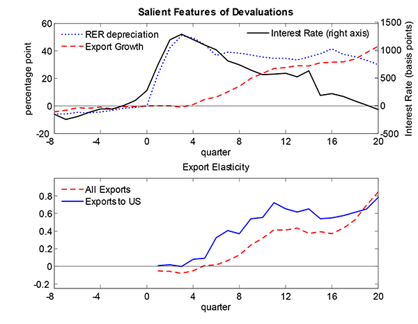
Figure 2: High Interest Rate Countries Versus Low Interest Rate Countries
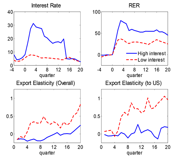
Figure 3A: Dynamics of Exports to US - Share Basis
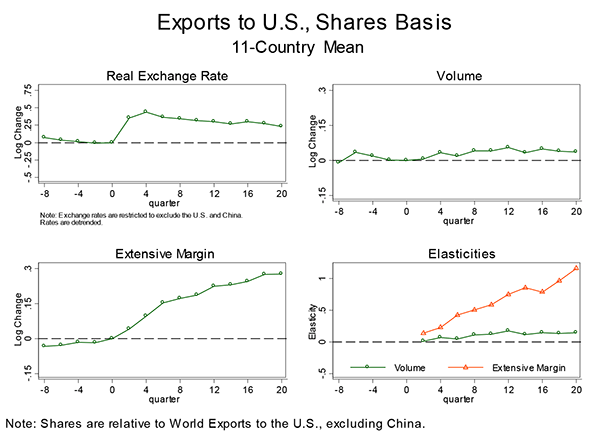
Figure 3B: Dynamics of Exports to US - Destrended
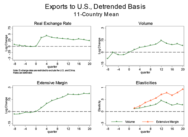
Figure 4: Exports to US by Interest Rate
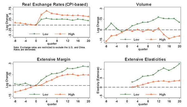
Note: Volume and Extensive margin are detrended
Figure 5: Share of Export Growth to US Accounted for by Extensive Margin
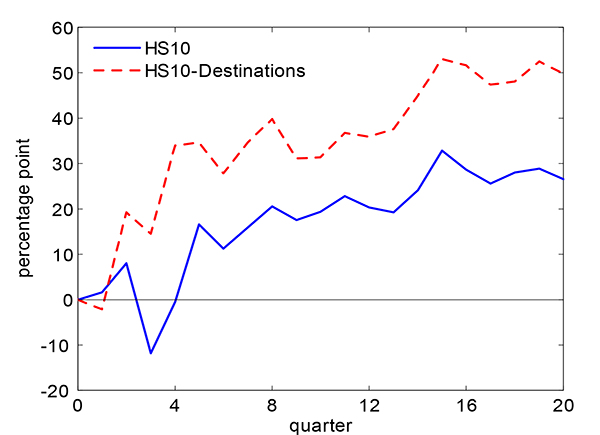
Figure 6: Decomposition of Export Growth by Extensive Margin Measures
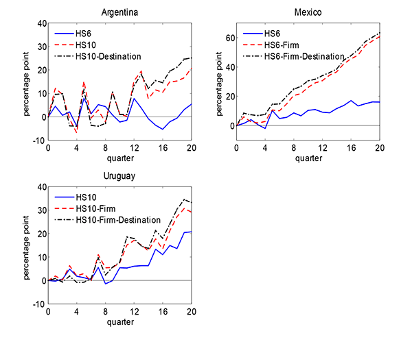
Figure 7: Aggregates in Data and Models
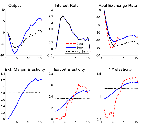
Figure 8: Productivity, Interest Rates, Discount factor, Labor Productivity
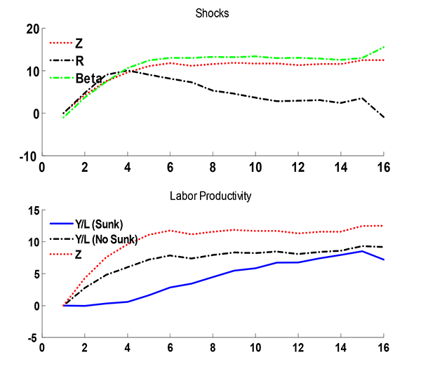
Figure 9: Impulse Response

Figure 10: Response to Di¤erent Interest Rates Paths
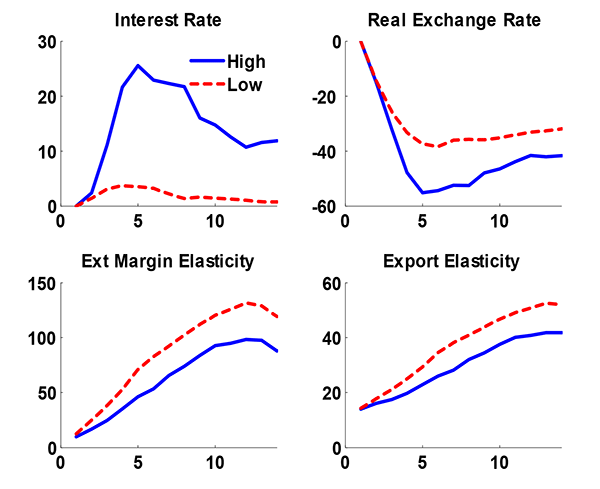
Figure 11: Sensitivity to Armington Elasticity and Elasticity of Substitution
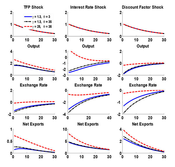
Figure 12: Making Exports Sluggish in No Sunk Cost Model
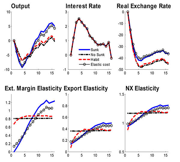
Figure 13: Sluggish Net Exports
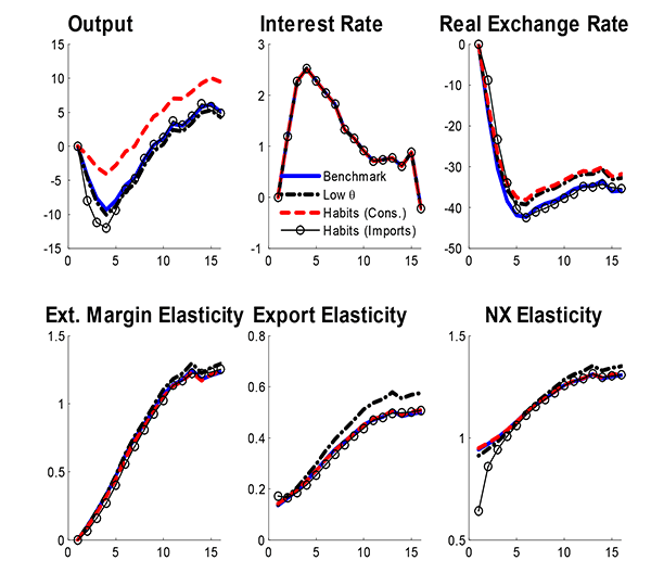
7 Appendix 1: The Export Supply Function
This appendix describes the derivation of export demand from the
ROW. In the ROW, final goods are produced using only home and
foreign intermediate goods (these are Argentinian goods). A final
good producer can purchase from any of the home intermediate good
producers but can purchase only from those foreign intermediate
good producers that are actively selling in the home market. In
each period there are
![]() identical foreign
intermediate producers selling in the home country.
identical foreign
intermediate producers selling in the home country.
The production technology of the firm is given by a constant elasticity of substitution (henceforth CES) function
| (19) | ![\begin{displaymath} D(s^{t})=\left \{ a_{1}\left[ \int_{0}^{1}y_{h}^{d}(i,s^{t})^{\frac{\theta -1 }{\theta }}di\right] ^{\frac{\theta }{\theta -1}\frac{\gamma }{\gamma -1} }+\left( 1-a_{1}\right) \left[ \int_{0}^{N\left( s^{t}\right) }y_{f}^{d}(i,s^{t})^{\frac{\theta -1}{\theta }}di\right] ^{\frac{\theta }{ \theta -1}\frac{\gamma -1}{\gamma }}\right \} ^{\frac{\gamma }{\gamma -1}}, \end{displaymath}](img226.gif)
|
where ![]() is the output of final goods and
is the output of final goods and
![]() and
and
![]() are inputs of
intermediate goods purchased from home firm
are inputs of
intermediate goods purchased from home firm ![]() and
foreign firm
and
foreign firm ![]() , respectively. The parameter
, respectively. The parameter
![]() determines the weight of home goods in
final good consumption. We will assume that
determines the weight of home goods in
final good consumption. We will assume that ![]() is
close to 1. The elasticity of substitution between intermediate
goods that are produced in the same country is
is
close to 1. The elasticity of substitution between intermediate
goods that are produced in the same country is ![]() , and the elasticity of substitution between home and
foreign aggregate inputs is
, and the elasticity of substitution between home and
foreign aggregate inputs is ![]() .
.
The final goods market is competitive. In each period
![]() , given the final good price at home
, given the final good price at home
![]() , the
, the ![]() home
intermediate good price at home
home
intermediate good price at home
![]() for
for
![]() , and the
, and the ![]() foreign intermediate good price at home
foreign intermediate good price at home
![]() for
for
![]() . A home final good
producer chooses inputs
. A home final good
producer chooses inputs
![]() for
for
![]() , and
, and
![]() for
for
![]() to maximize
profits,
to maximize
profits,
| (20) | 
|
Solving the problem in (20) gives the input demand functions,
| (21) | ![$\displaystyle a_{1}^{\gamma }\left[ \frac{P_{h}(i,s^{t})}{ P_{h}(s^{t})}\right] ^{-\theta }\left[ \frac{P_{h}(s^{t})}{P(s^{t})}\right] ^{-\gamma }D(s^{t}),$](img251.gif)
|
||
| (22) | ![$\displaystyle \left( 1-a_{1}\right) ^{\gamma }\left[ \frac{ P_{f}(i,s^{t})}{P_{f}(s^{t})}\right] ^{-\theta }\left[ \frac{P_{f}(s^{t})}{ P(s^{t})}\right] ^{-\gamma }D(s^{t}),i\in \left[ 0,N\right] ,$](img254.gif)
|
where
![$P_{h}(s^{t})=\left[ \int_{0}^{1}P_{h}(i,s^{t})^{1-\theta }di\right] ^{ \frac{1}{1-\theta }}$](img255.gif) , and
, and
![$P_{f}(s^{t})=\left[ \int_{0}^{N}P_{f}(i,s^{t})^{1-\theta }di\right] ^{\frac{1}{1-\theta }}$](img256.gif) . The zero-profit condition in the perfectly competitive market
determines the price level of the final good as
. The zero-profit condition in the perfectly competitive market
determines the price level of the final good as
| (23) | ![\begin{displaymath} P(s^{t})=\left[ a_{1}^{\gamma }P_{h}(s^{t})^{1-\gamma }+\left( 1-a_{1}\right) ^{\gamma }P_{f}(s^{t})^{1-\gamma }\right] ^{\frac{1}{1-\gamma }}. \end{displaymath}](img257.gif)
|
Now we are assuming that we have N identical exporters, each
charging
![]() and so
and so
 . Aggregating over the different exporters we get
![\begin{eqnarray*} EX\left( s^{t}\right) &=&\int_{0}^{N\left( s^{t}\right) }y_{f}^{d}(i,s^{t})=\int_{0}^{N\left( s^{t}\right) }\left( 1-a_{1}\right) ^{\gamma }\left[ \frac{P_{f}(i,s^{t})}{P_{f}(s^{t})}\right] ^{-\theta }\left[ \frac{P_{f}(s^{t})}{P(s^{t})}\right] ^{-\gamma }D(s^{t}) \ &=&N\left( s^{t}\right) \left( 1-a_{1}\right) ^{\gamma }\left[ \frac{ P_{f}(i,s^{t})}{P_{f}(s^{t})}\right] ^{-\theta }\left[ \frac{P_{f}(s^{t})}{ P(s^{t})}\right] ^{-\gamma }D(s^{t}) \ &=&N\left( s^{t}\right) \left( 1-a_{1}\right) ^{\gamma }\left[ \frac{1}{ N\left( s^{t}\right) ^{\frac{1}{1-\theta }}}\right] ^{-\theta }\left[ \frac{ N\left( s^{t}\right) ^{\frac{1}{1-\theta }}p_{f}\left( s^{t}\right) }{ P(s^{t})}\right] ^{-\gamma }D(s^{t}). \end{eqnarray*}](img260.gif)
Now let's take log deviations from the
![\begin{displaymath} \ln EX\left( s^{t}\right) \propto \ln \left[ \frac{\left( 1-a_{1}\right) \left( \theta -1\right) }{\theta }\right] +\frac{1-\gamma }{1-\theta }\ln N\left( s^{t}\right) -\gamma \ln \left[ \frac{p_{f}\left( s^{t}\right) }{ P(s^{t})}\right] +\ln D(s^{t}). \end{displaymath}](img261.gif)
Let's define the terms of trade ![]()

then we can rewrite log deviation of export demand as

In terms of revenue

Appendix 2: Data sources
7.1 Macro Data
- Exchange rates: The real exchange rate was calculated as
where

 is the nominal exchange rate of
country
  at time
  . These three series
were obtained from the International Financial Statistics (IFS)
database published by the International Monetary Fund. All price
indices have the base year 2005.
 - Total exports and imports are from the IFS database in millions of US dollars.
- Exports and imports to the US: Total exports (FAS value) in millions of dollars are from the Haver US International Database. Imports (customs value) are in millions of dollars.
- US import price deflator for non-petroleum goods (2005=100) are from the Haver US International Database.
- Interest Rates: We use the following interest rates for each
country:
- JP Morgan EMBI+ Stripped Spread. for Argentina, Colombia, Mexico, and Turkey
- JP Morgan EMBI Global Stripped Spread for Brazil, Korea, Malaysia, Russia, Thailand, and Uruguay
- Since the EMBI Spread data for Indonesia were not available for the period around the crisis period we used the Indonesia Republic 7 3/4 Stripped Spread that matured in 2006.
- US real expenditure measured as an average of US industrial production (IP) and US real imports of nonpetroleum goods (SAAR, Bil.Chn.2005$)
- Foreign real expenditure
 measured as an
average of World IP (Haver) and US real imports.
 - Country-level output from Figure 7 on is based on industrial production (IFS, except for Colombia which is DANE). A linear trend has been removed from country-level output.
7.2 Bilateral Data
- Disaggregated shipment data on imports from all countries to the US were obtained from the US Census Bureau Merchandise Trade CDs. This data set breaks down US imports by HS 10 commodity, country of origin and port of entry.
- Imports in US dollars were deflated by the US import price deflator for non-petroleum goods. Only manufacturing goods imports were considered. Manufactured goods were defined as HS-10 goods that were concorded to SITC 5-8.
- Restricted Real Exchange Rates
- Trade weights are taken from the JP Morgan Broad Index Trade Weights based on 2000 trade in manufactured goods, available from Haver's website. Trade weights are not available for Uruguay, so we did not make the trade-weighted real exchange rate calculation for it.
- For any country
 , let
, let  be
the trade-weighted real exchange weight measured in log changes.
For any countries
  and
and  , let
, let
 be the trade weight, measuring
the fraction of
  trade that is with
 . For any countries/parts of the world
 and
and  , let
, let  be the real exchange rate between
  and
and  , measured in log changes. Now, let
 be the country whose RER we are looking to
restrict, and let ROW be the world, excluding
  ,
the US, and China (C). Then we calculated the restricted real
exchange rate as:

7.3 Country-Level Customs Data
The data for Argentina and Uruguay were obtained from Penta Transactions, a commercial data provider.
- The Argentina data are comprised of exports of all HS 11 products, disaggregated by destination country at a daily frequency from January 2000 to December 2011. Exporter information was provided for some periods but not consistently around the crisis and sit was not used.
- The Uruguay data contained exports of all HS 10 products, denominated in US dollars, disaggregated by exporter and destination country at a daily frequency from January 2000 to December 2011.
- The data for Mexico were provided by the Mexican Finance Ministry. It contains information on Mexican exports at a quarterly frequency from 1993Q1 to 1999Q4. Exports were disaggregated by HS 6 products, exporter ID and country of destination.
In each database, manufacturing exports (HS10 codes concorded to SITC 5 to 8 codes) were selected. All exports were in US dollars and were deflated using the US import price deflator for non-petroleum goods.
Appendix Figure 1A: Real Exchange Rates
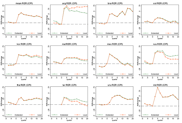
Appendix Figure 1B: Exports to U.S.
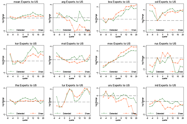
Appendix Figure 1C: Extensive Margin of Exports to U.S.
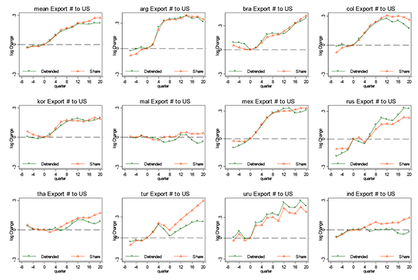
Footnotes
1. Alessandria: Federal Reserve Bank of Philadelphia, Ten Independence Mall, Philadelphia, PA 19106 ([email protected]); Pratap: Department of Economics, Hunter College and the Graduate Center City University of New York Room 695 Park Ave, New York, NY 10065 ([email protected]); Yue: Federal Reserve Board of Governors, 20th and Constitution Ave, Washington DC 20551 ([email protected]). We thank Luigi Bocola, Svetlana Chekmasova, and Oscar Puente for excellent research assistance. We also thank Costas Arkolakis, Ariel Burstein, Lukasz Drozd, Brent Neiman, Francesco Pappada, John Romalis, Kim Ruhl, Mike Sposi, and the participants at the Atlanta Fed-NYU confererence, BU, ECB-Bank of Canada Workshop on Exchange Rates, New York Fed, NYU, Federal Reserve Board, Paris School of Economics, HEC-Montreal, INSEAD, IMF, ITAM, Ohio State University, Richmond Fed, Stonybrook, Tsinghua Macro Workshop, Econometric Society Annual meeting, LACEA-IDB-CAF Trade, Integration, Growth Conference, American Economic Annual Meeting, and the Society of Economic Dynamics Annual Meeting. We are grateful to Lorenza Martinez and Kensuke Teshima for the use of Mexican customs data. The views expressed herein are those of the authors and should not be interpreted as reflecting the views of the Federal Reserve Bank of Philadelphia or the Board of Governors or any other person associated with the Federal Reserve System. Return to text
2. An example of this sluggishness is from the lierature on the J-curve (Magee, 1973, Junz and Rhomberg, 1973, Meade, 1988 and Backus, Kehoe and Kydland 1994). Return to text
3. Manova (2013) studies the role of credit constraints on firm level exporting decisions. Return to text
4. More generally, it is well known that trade tends to respond with a lag to real exchange fluctuations. That is, the estimates of the short-run trade elasticity are smaller than the long-run trade elasticity. An advantage of focusing on large devaluations is that they provide an estimate of the time it takes for trade to respond. Return to text
5. The export elasticity is measured as the change in the ratio of exports to foreign expenditures divided by the change in the real exchange rate, where the changes are calculated relative to their pre-devaluation levels. It is a convenient way to compare the export response in countries with devaluations of different sizes. Return to text
6. By the Melitz model, we mean the standard version with no plant dynamics and no distinction between startup and continuation costs, resulting in a static export decision.
7. In these models, interest rates can affect trade through general equilibrium factors. In particular, a rise in world interest rates encourages savings, which can stimulate exports. This makes the finding of a negative relationship between interest rates and exports even more puzzling. Return to text
8. Shocks to the discount factor are commonly employed in macro models to generate financial crises such as the Great Recession or Japan's liquidity trap (Eggertsson and Woodford, 2003). Return to text
9. We consider additional features related to output and net exports when we examine the model's properties. Return to text
10. We focus on this measure of trade flows since it allows us to compare the export response of devaluations of different sizes. In standard theories (Backus, Kehoe, and Kydland, 1994) this variable is directly related to the Armington elasticity. Return to text
11. We also measure interest rates using the financing cost for the edian firm based on the World scope data at the annual frequency. For periods after 2003, JP Morgan also provides the Corporate EMBI spreads. The correlation between EMBI and these alternative interest rate measures for the overlapping periods is high and significant. Return to text
12. Foreign expenditure is measured as an average of world industrial production and trade. Return to text
13. In an Armington trade model this elasticity is closely related to the elasticity of substitution between imports and domestic goods and is constant. Return to text
14. For each country we compute a weighted average of the increase in the interest rate over the first 12 quarters following the devaluation. The earlier periods are weighted mroe heavily than later periods. We then compute the median increase in interest rates. Countries with interest rates that increased more than the median are classified as high interest rate countries. The remaining countries are classified as low interest rate countries. Our decomposition into high and low interest rate countries is fairly robust to our weighting scheme, interval considered (i.e. the period over which the average was computed), or measure studied (financing cost for median firms or EMBI spreads). Return to text
15. We exclude Mexico from the analysis of differential export responses to changes in interest rates given its integration with the US. Return to text
16. This does not fully capture the potential changes in exports, since changes in relative prices could also lead to a change in the share of imports in US expenditures. However, this effect is small since devaluing countries have a small impact on the relative price of imports to domestic expenditures. Return to text
17. Each country's industry import trade
weights are based on 10-year window around the devaluation
![]() Return to text
Return to text
18. Our measure of the extensive margin is the average number of HS10-districts per month. Return to text
19. Figure 4 is based on the detrended data where the trade is calculated using the full sample for individual countries. The difference in the extensive margin is more pronouced before detrending or using the pre-devaluation trend. Return to text
20. An alternative decomposition is to define continuers, entrants, and exiters period by period and calculate the intensive and extensive margin, as in Eaton et al. (2007). Return to text
21. Discount factor shocks are common in
macroeconomic modelling (see Eggertsson and Woodford, 2003, Smets
and Wouters, 2007, Guerron, 2010, and Christiano, Eichenbaum, and
Rebelo, 2011). An increase in ![]() will generate a
sudden stop in that it will lead to a large increase in the current
account and a large depreciation. In this respect it is similar to
a shock that tightens a borrowing constraint (Mendoza,
2010). Return to text
will generate a
sudden stop in that it will lead to a large increase in the current
account and a large depreciation. In this respect it is similar to
a shock that tightens a borrowing constraint (Mendoza,
2010). Return to text
22. We focus on these shocks rather than shocks to foreign demand or the exogenous price of exports. Return to text
23. This is a parsimonious way of modelling the differences in tradables and nontradables as well as allowing the model to generate fluctuations in producer and consumer prices. Return to text
24. Any other way of making the economy stationary is fine too. See Schmitt-Grohe and Uribe (2003) for alternative methods to close the small open economy models. We assume agents do not internalize the effect of their borrowing on the risk premium so that our results do not depend on whether the increase in interest rates is from the country spread or the world rate. Return to text
25. We focus on a model with no dispersion in exports among exporters. We have also developed a model in which new exporters start exporting a small amount and expand exports gradually over time. This richer model generates a nearly identical aggregate response to the shocks considered, so we focus on this more parsimonious model. Return to text
26. We take this approach since the shocks in the periods that we concentrate on are quite different from the entire time series. Return to text
27. We remove a log-linear trend from real output. Return to text
28. In the data we proxy D with a measure of industrial production. Return to text
29. A convenient feature of this way of modeling habit is that it does not change our measure of prices. Return to text
This version is optimized for use by screen readers. Descriptions for all mathematical expressions are provided in LaTex format. A printable pdf version is available. Return to text