Board of Governors of the Federal Reserve System

August 29, 2018

The Monetary Policy Response to Uncertain Inflation Persistence

Robert Tetlow¹

1. Introduction
A critical component of the design of monetary policy is policymakers' perception of the persistence of inflation, either on its own, or as a proxy for the behavior of long-term inflation expectations. If inflation can be taken to be "well anchored," then shocks to inflation will have a tendency to die out rapidly, ameliorating the need for a monetary policy response to offset the shock. If, on the other hand, inflation is persistent, then inflation expectations are not well anchored; shocks are said to work their way into inflation expectations and are thus persistent in their effects, obliging an offsetting policy response.² But inflation persistence is not a fixed parameter. As a statistical phenomenon, inflation has evolved over time in a manner that suggests that policymakers cannot take for granted any estimate of its persistence.

This FEDS Note considers the implications of uncertainty regarding the persistence of inflation for the conduct of monetary policy. Inflation persistence is a special case of a much studied and more general question of the optimal policy response to parameter uncertainty. The extent to which long-term inflation expectations are "well anchored," is an interesting question, partly because of the primacy of the issue, but also because the results in this instance are different from what some observers might expect and yet have an intuitive interpretation. The seminal paper of Brainard (1967) has made policymakers comfortable with the presumption that uncertainty about the parameters in the economy implies attenuation in policy responses--that is, less vigorous policy feedback--relative to the optimal policy when the parameter in question is fixed and known. Indeed, Alan Blinder noted that the Brainard result was "never far from my mind when I occupied the Vice Chairman's office at the Federal Reserve. In my view…a little stodginess at the central bank is entirely appropriate" (Blinder, 1988, p. 12). We will show that the Brainard attenuation principle does not hold for the case of inflation persistence.

2. Optimizing policy under parameter uncertainty: the Bayesian case
2.1 A very simple model

Throughout, we assume that policy is governed by a Taylor rule, the coefficients of which we shall optimize; the question will be what values for the feedback coefficients in the rule produce the best economic performance, given uncertainty.³ Most of the analysis is carried out using the Bayesian approach to uncertainty meaning that policymakers are assumed to have a well identified set of prior beliefs regarding possible parameter values. However, we offer at the end a short discourse on the Knightian approach to uncertainty, where the uncertainty is said be accompanied by ambiguity in that priors are not well defined in the Bayesian sense.⁴

To make things concrete, we employ a very simple linear model of New Keynesian flavor:

(1)      $$$ \pi _{t} =\beta \cdot \pi _{t-1}^{4} +\kappa \cdot y_{t} +\sigma _{\pi } \cdot u_{t}$$$
(2)      $$$ y_{t} =\alpha \cdot E_{t} y_{t+1} +(1-\alpha )\cdot y_{t-1} -\gamma \cdot (rn_{t} -E_{t} \pi_{t+1}^{4} )+\sigma _{y} \cdot \varepsilon_{t}$$$
(3)      $$$ rn_{t} =\phi_{y} y_{t} +\phi_{\pi } \pi _{t}^{4}$$$

where π is quarterly inflation measured at annual rates; π⁴ is four-quarter inflation; y is the output gap; rn is the policy rate, measured at annual rates; u, ε are shocks distributed normally and independently with unit variances, and Γ = [ β,κ, α, γ, σ_π, σ_y, ϕ_y, ϕ_π ] are parameters. We think of $$\beta \cdot \pi^{4}$$ as capturing wage and price setters' conception of expected inflation. Qualitatively speaking, nothing that follows depends on parameter values, so long as those parameters fall within a broad set; in any event, the parameters used here are based largely on simple regressions, and are as follows: β = 0.88; κ = 0.025; α = 0.2; γ = 0.3; σ_y = 0.5; σ_π = 0.5.

2.2 Policy preferences and prior beliefs

The parameters noted above omitted those of the Taylor-type rule, equation (3). These parameters are chosen using well-known computational methods to minimize a standard quadratic loss function:

(4)      $$$ L=\sum _{i=0}^{\infty }\rho ^{i} \cdot [0.25\cdot y_{t+i}^{2} +1\cdot \pi _{t+i}^{2} +0.1\cdot (rn_{t+i} -rn_{t+i-1} )^{2} ] $$$.

We think of the loss function, equation (4), as consistent with the Federal Reserve's "dual mandate" as specified in legislation, as well as with the "balanced approach" to policy the FOMC has described in its "Statement of Longer-Run Goals and Monetary Policy Strategy". This is because the weight of 0.25 on the output gap in equation (4) is roughly equivalent to a loss function that has a weight of unity on the deviation of the unemployment rate from its natural rate, translated into output gap terms assuming an Okun's Law coefficient of two. Equation (4) also includes a term in the change in the policy rate, with a small weight, customary in such problems and necessary to obtain empirically plausible policy behavior. In our normative analysis, we will evaluate economic performance omitting the term in the change in policy rate, although results turn out to be the same either way.

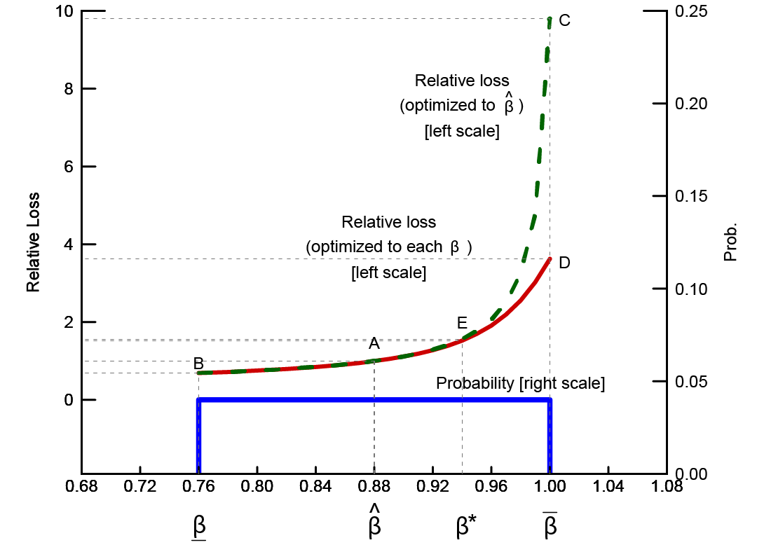
The key parameter is β which can be thought of as capturing the extent to which inflation expectations are "well anchored." If β << 1, shocks to equation (1) will tend to die out rapidly, independent of policy actions; however, as β →1, shocks to equation (1) will tend to persist, and in the limit when β = 1 the model becomes "accelerationist," meaning that temporary shocks have permanent effects on inflation, all else equal. Policymakers take the inflation-persistence parameter, β, as unknown but believe that the true value lies in a uniform distribution, $$\beta \subset (\underline{\beta },\overline{\beta })$$ with $$E\beta \equiv \widehat{\beta} =$$ 0.88, $$\underline{\beta} =$$ 0.76, , $$\overline{\beta} =$$ 1. The blue rectangle at the bottom of figure 1 shows the uniform distribution of values for β, with the probabilities read off of the right-hand scale.

Figure 1: Economic Losses as a Function of Inflation Persistence (optimized Taylor rule; simple model example)

2.3 Results

The red solid line in figure 1 shows economic losses for the hypothetical case in which policymakers know the true value of β and the policy rule coefficients in equation (3) have been optimized for each of the possible values. The upward slope in the red line demonstrates that increased inflation persistence is costly from policymakers' perspective, even when the persistence parameter is known. The green dashed line shows economic performance of the model when the policy rule coefficients have been optimized for the expected (mean and median) value, $$E\beta \equiv \widehat{\beta } =$$ 0.88 but where the actual value of β is allowed to vary over the range shown. This is the policy that would be chosen by policymakers who ignore parameter uncertainty; that is, they are following a certainty equivalent policy. Note that on the green line, point A is the only point at which the policy rule coefficients have been optimized for the correct parameter value.

Uncertainty over inflation persistence is multiplicative in the sense that the model cannot be rewritten such that β is a stand-alone (additive) term. This means that certainty equivalence will not be the best response to uncerntainty, in general. Risk management considerations should be expected to result in a departure from certainty equivalence, even though policymakers' preferences are quadratic, the model is linear, and shocks are normally distributed. Point B, also on the green dashed line, shows the loss that is incurred when the inflation persistence parameter turns out to be at the low end of the range, that is, $$\beta =\underline{\beta } = $$ 0.76. As can be seen, when inflation is less persistent, economic performance improves, relative to point A, even though policymakers in this instance conduct policy with a rule that is based on the wrong value of β. By contrast, at point C, when $$\beta =\overline{\beta } = $$ 1.00, economic performance is substantially worse, given policymakers' treatment of $$\beta =\widehat{\beta}$$. It follows that if policymakers were to choose to ignore the uncertainty in their estimate of β, economic risks would not be balanced. What this simple example highlights is that even though errors in the estimation of β are symmetrically distributed around policymakers' best guess, economic losses associated with those values are not symmetric.

Figure 2: Optimized Taylor Rule Coefficients as a Function of Inflation Persistence (simple model example)

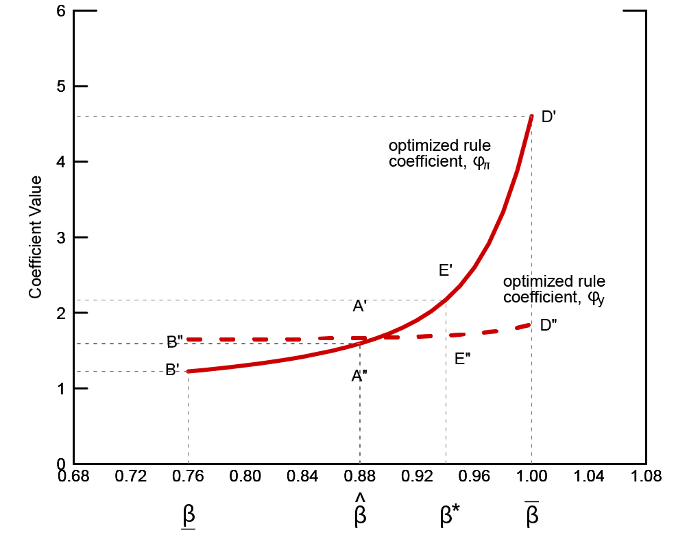
Figure 2 shows the rule coefficients, optimized as a function of β. The optimized coefficients for our base case, $$\beta = \widehat{\beta}$$ are $$[\phi_{\pi } ,\phi _{y} ] = $$ [1.59, 1.67]. While we would not want to make much of these particular coefficients, optimized as they are for what is essentially a toy model, they are close to those of the Taylor (1999) rule. As one might expect, the optimized coefficient on inflation, ϕ_π is strongly increasing in β; the coefficient on the output gap, ϕ_y, also increases with β, but only slightly. Suppose $$\beta =\overline{\beta} =$$ 1.00. If policymakers knew this, they could substantially improve economic performance as shown by the distance from point C to point D in figure 1. But note that there is no corresponding prospect for improvement at the lower end of the range. It follows that the optimal policy under uncertainty is for policymakers to adjust their working estimate of inflation persistence such that the probability-weighted loss for the range of values for β is minimized; this results in a choice of $$\beta =\beta^{*} \approx $$ 0.94 $$>\widehat{\beta}$$, which delivers expected performance shown by point E on the red line in figure 1. The logic is simple: because underestimating β is more costly than overestimating it, the best response to uncertainty is to lean toward higher values. One implication of this observation is rhetorical: it is not generally correct to associate caution in monetary policy design with attenuation, or gradualism; sometimes the cautious response is a more aggressive response.

Also notice from figure 2 that the policy rule parameterization implied by this risk management is more aggressive; that is to say, coefficients E' and E'' are larger than they are for the certainty equivalent policy, points A' and A''. Thus, we uncover an instance in which the logic of Brainard (1967), according to which the optimal response to uncertainty is to attenuate policy feedback relative to the certainty equivalent case, does not hold. Although we will not devote space to the topic here, it is the case that the best response to uncertainty for many other parameters is either no change in feedback--that is, certainty equivalence--or attenuated policy.

3. Optimizing policy under parameter uncertainty: the robust case

The foregoing has described how policymakers who have well-defined (Bayesian) priors over inflation persistence respond to uncertainty by minimizing the probability-weighted expected loss. There are instances, however, in which policymakers may be unwilling or unable to assign probabilities over the complete set of possible outcomes. In those instances, the literature prescribes practicing ambiguity aversion. The literature on ambiguity aversion is large and sprawling; we cannot do justice to it here. We can, however, give a flavor of the approach by considering a particular special case. Suppose our policymakers retain their view that $$\beta \subset (\underline{\beta },\overline{\beta})$$, but that they are unwilling or unable to assign probabilities for β within that range. Under these circumstances, the literature says that policymakers should act as though the true value of β is the one that delivers the worst-case loss within the range, so as to hedge against that outcome. In other words, policymakers minimize the maximum loss that they believe they could incur. In this simple model, and with ambiguity confined to just this one parameter, loss is strictly increasing in β, so robust policymakers would choose $$\beta^{r} =\overline{\beta}$$, which in turn means selecting rule parameters D' and D''. This outcome reflects policymakers' distrust of expressions for likelihood for values for $$\beta <\overline{\beta }$$. More generally, the ambiguity-adverse approach to uncertainty tends to produce anti-attenuation outcomes, like the one just described, with greater frequency than does the Bayesian approach.

4. Concluding remark

This Note has considered a special case of parameter uncertainty and its implications for the design of monetary policy. We have shown that the proper response to uncertainty concerning inflation persistence is not the customary policy attenuation, in the sense of Brainard (1967), but rather anti-attenuation, meaning a more aggressive response to inflation than is the case when the inflation persistence parameter is known. More generally, we have shown that what should be of primary interest to policymakers is not so much what values the true parameter could turn out to be, but rather the damage to their goals that might be incurred, given those parameter values.

References:
Bernanke, Ben S. (2017) "Monetary Policy under Uncertainty" speech given to the 32^nd Annual Economic Policy Conference, Federal Reserve Bank of St. Louis. October 19.

Blinder, Alan S. (1998) Central Banking in Theory and Practice Cambridge, MA: MIT Press.

Brainard, William (1967) "Uncertainty and the effectiveness of policy" 57, American Economic Review, 2 (May): 411-425.

Ellison, Martin and Thomas J. Sargent (2012) "A Defense of the FOMC" 53, International Economic Review, 4 (November): 1047-1065.

Hansen, Lars P. and Thomas J. Sargent (2008) Robustness Princeton: Princeton University Press.

Hansen, Lars P. and Thomas J. Sargent (2015) "Four types of ignorance" 69, Journal of Monetary Economics, 1 (January): 97-113.

Söderström, Ulf (2002) "Monetary policy with uncertain parameters" 104, Scandinavian Journal of Economics, 1: 125-145.