IFDP Notes
May 15, 2017
Milton Friedman and Data Adjustment
Neil R. Ericsson, David F. Hendry, and Stedman B. Hood1
When empirically modelling the U.S. demand for money, Milton Friedman more than doubled the observed initial stock of money to account for a "changing degree of financial sophistication" in the United States relative to the United Kingdom. This note discusses effects of this adjustment on Friedman's empirical models. His data adjustment dramatically reduced apparent movements in the velocity of circulation of money, and it adversely affected the constancy and fit of his estimated money demand models.
1. Introduction
Monetarism has experienced a resurgence of interest in the economics profession, as highlighted by Benati, Lucas, Nicolini, and Weber's (2017) VoxEU column and Cord and Hammond's (2016) book commemorating Milton Friedman. Drawing on Ericsson, Hendry, and Hood (2016), the current note re-examines Milton Friedman's empirical methodology, focusing on his modelling of the U.S. demand for money in Friedman and Schwartz (1982). Specifically, we consider three related issues.
- Data adjustment for changing financial sophistication and cyclical variability
- Model constancy
- Measured goodness of fit
We find that Friedman and Schwartz's final money demand models suffer from substantive empirical shortcomings, despite their adjusting a third of the observations to reflect changing financial sophistication and smoothing all the data over phases of the business cycle. Estimated income and interest-rate elasticities differ markedly over subsamples, and the reported empirical models substantially overstate goodness of fit. These properties are problematic for Friedman's monetarism.
2. Friedman: Statistician and Economist
Early in his career, Friedman made original contributions to several areas of statistics. For example, he derived a test for subsample constancy, solved a small-sample testing problem for ranks, and developed sequential sampling procedures. As an economist, Friedman focused on understanding money and its roles in the economy--a lifelong research activity for him. The three books that he co-authored with Anna Schwartz are milestones in that endeavor. Friedman and Schwartz (1963, 1970) provided comprehensive historical, institutional, narrative, and statistical underpinnings for the U.S. data subsequently analyzed in Friedman and Schwartz (1982), denoted FS hereafter. Data and their treatment occupied a central role in that research. Our focus is Friedman and Schwartz's data (which span 1867–1975), and FS's analysis of those data.
3. Data Adjustment
We begin with the issue of data adjustment. FS were primarily interested in longer-run trend behavior. FS also recognized the importance of institutional and other changes for the relationships that they modelled. To capture such effects, FS employed data adjustment, specifically addressing both changing financial sophistication and cyclical variability.
Concerning financial sophistication, FS perceived an initial lack of variety and extent of instruments and institutions in the financial system in the United States, relative to those in the United Kingdom, but with subsequent rapid developments in the United States. FS characterized this as a "changing degree of financial sophistication" FS (p. 221). FS accounted for these developments prior to modelling money demand by adjusting the U.S. money stock series by a linear trend of 2.5% per annum for observations before 1903, with no trend adjustment thereafter; FS (p. 217). Consequently, while the unadjusted money stock for 1867 is $1.28 billion, its adjusted value is $3.15 billion: 246% of its original value. This adjusted series features prominently in FS's analysis of U.S. monetary behavior. It is used to construct a key variable in their analysis--the velocity of circulation of money, or "velocity"--which is the ratio of nominal income to nominal money.2 FS also used the adjusted series for the money stock to construct the dependent variable for their U.S. money demand models.
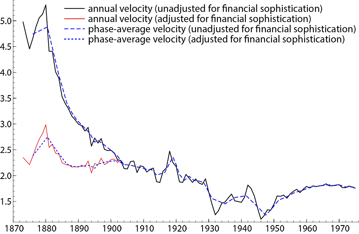
Figure 1 plots unadjusted and adjusted velocity using FS's annual data, and the adjustment is large.
This adjustment is important since it accounts for almost three quarters of the total variance of velocity in the whole period [FS] cover, even though the adjustment itself applies to only 30 percent of the period. Mayer (1982, p. 1532), emphasis added
This data adjustment materially alters the properties of the data, such as of velocity. FS believed that velocity is reasonably constant empirically.
... a numerically constant velocity does not deserve the sneering condescension that has become the conventional stance of economists. It is an impressive first approximation that by almost any measure accounts for a good deal more than half of the phase-to-phase movements in money or income. Almost certainly, measurement errors aside, it accounts for a far larger part of such movements than the other extreme hypothesis--that velocity is a will-o'-the-wisp reflecting independent changes in money and income. FS (p. 215)
Surprisingly, FS's data don't support the view that velocity is relatively constant. As Figure 1 shows, unadjusted velocity falls by more than two thirds from the 1870s to the 1940s. Although adjustment for changing financial sophistication dramatically increases the apparent constancy of velocity, adjusted velocity still falls by half over the same period.3
The adjustment for changing financial sophistication raises several issues.
- It is unclear why the initial lack of U.S. financial sophistication should be judged relative to financial sophistication in the United Kingdom, rather than relative to that in some other country; or why a constant improvement of 2.5% per annum is appropriate.
- It is not obvious why financial sophistication in the United States caught up to that in the United Kingdom in precisely 1903, even though the international role of the dollar continued increasing relative to that of sterling throughout the 1900s.
- Other variables such as interest rates and income might have been affected by changing financial sophistication, but they were not adjusted for it.
FS also employed data adjustment to remove cyclical variability. FS averaged their annual data over phases of the business cycle--that is, separately over expansions and contractions. Phase averaging does reduce higher-frequency fluctuations in the annual data, mainly at the start of the sample and again during the Great Depression and WWII. However, phase averaging does not fully eliminate the data's short-run movements. Figure 1 portrays this evidence in graphs of annual and phase-average values of velocity. Overall, the annual and phase-average data series move closely together.
In addition to affecting data properties, data adjustment altered inferences in FS's estimated models, as we now discuss for empirical model constancy and goodness of fit.
4. Evaluating Friedman and Schwartz's U.S. Money Demand Models
FS were concerned about the empirical constancy of models estimated on the adjusted data. Hence, we replicated FS's U.S. phase-average money demand models. Using the approach in Hendry, Johansen, and Santos (2008)--as implemented in Doornik and Hendry's (2013) econometrics software package OxMetrics--we detected significant shortcomings, including residual autocorrelation and parameter nonconstancy in their final log-levels money demand model. That nonconstancy can be characterized by numerically large and highly significant impulse indicator dummies for business-cycle phases corresponding to 1878–1882, 1932–1937, and 1944–1946. Each of these indicators captures a shift of approximately 15% of the adjusted money stock.
Even with the (pre-1903) adjustment for financial sophistication, FS's final log-levels phase-average model fits appreciably worse on the full sample than on just the post-1903 data, which have no adjustment for financial sophistication. Moreover, the estimated trend is more than 4% on the pre-1903 data for that model, contrasting with FS's imposed adjustment of 2.5% over the same period. Income and interest-rate elasticities differ markedly for models estimated on pre- and post-1903 data.4
As Figure 1 highlights, FS's adjustment for financial sophistication makes velocity look more constant. However, that adjustment does not adequately capture the changes that occurred. Notably, one of FS's key criteria is model constancy, yet their money demand models fail on that measure.
Although not an aspect of data adjustment per se, Friedman's empirical methodology emphasizes a simple-to-general modelling approach--estimating many simple empirical models in order to build a picture of a more complicated relationship. Friedman and Schwartz's final money demand equations are the culmination of evidence from hundreds of simpler regressions--in Friedman and Schwartz's own words, "by examining variables one or two at a time" FS (p. 215). However, this simple-to-general approach is flawed when applied to high-dimensional, dynamic, nonstationary data that are subject to sudden and unanticipated shifts--data such as theirs, and irrespective of their data adjustment.
Friedman's empirical methodology also affected FS's final U.K. phase-average money demand models, which Hendry and Ericsson (1991) showed are nonconstant. Using an alternative methodological approach, general-to-specific modelling, Hendry and Ericsson (1991) then obtained a money demand model on FS's U.K. annual data that is empirically constant, well-specified statistically, and interpretable economically. Escribano (2004) updated that money demand model and showed that it remains empirically constant on more recent data. Methodology matters.
5. Comparing Goodness of Fit Across Models
FS were also concerned about a model's goodness of fit. Here, the key aspect is calculation of the residual standard error "σ", which measures what's not explained by a model. Proper calculation of σ reverses rankings of models previously estimated on FS's annual and phase-average data.
A brief digression may help clarify how to calculate σ for annual and phase-average models. In estimating their phase-average models, FS corrected for the heteroscedasticity that arose from averaging annual data over business-cycle phases that have different durations--in effect, estimating their models using weighted least squares. As Ericsson, Hendry, and Hood (2016) showed, the σ's from FS's heteroscedasticity-corrected phase-average models must therefore be rescaled to make those σ's comparable with each other, and with σ's from corresponding annual models.5 Rescaling factors for the σ's depend on the business-cycle phase lengths and the type of model (for instance, log-levels or rates of change).
FS did not rescale the σ's for their phase-average models. Hence, those σ's are not directly comparable with each other, or with σ's from annual models. Moreover, rescaling factors for FS's final phase-average models range from 1.7 to 8.0, which implies substantial overstating of those models' goodness of fit.
Table 1: Comparison of the residual standard error σ across money demand models. Source: Ericsson, Hendry, and Hood (2016).
| Country | Frequency | Model | Reported σ | Rescaling factor | Rescaled σ |
|---|---|---|---|---|---|
| United States | Phase | FS log-levels | 5.09% | 1.72 | 8.75% |
| Phase | FS rates of change | 1.48% | 5.44 | 8.05% | |
| Annual | Random walk of unadjusted velocity | 6.69% | 1 | 6.69% | |
| United Kingdom | Phase | FS log-levels | 5.54% | 1.85 | 10.25% |
| Phase | FS rates of change | 1.34% | 7.99 | 10.71% | |
| Annual | Random walk of velocity | 4.72% | 1 | 4.72% | |
| Annual | Hendry and Ericsson (1991, eq. (10)) | 1.42% | 1 | 1.42% |
Table 1 illustrates why rescaling is necessary. The first row records FS's reported value of σ for their final phase-average log-levels money demand model, that model's rescaling factor for σ, and the resulting rescaled value of σ. The reported σ and its rescaling factor are 5.09% and 1.72 respectively; and the rescaled σ is their product, namely, (5.09%x1.72), or 8.75%. The second row in Table 1 records the reported σ (1.48%), its rescaling factor (5.44), and the rescaled σ (=1.48%x5.44, or 8.05%) for FS's final phase-average money demand model in rates of change. Thus, two values of σ appear far apart as reported (5.09% and 1.48%) but, when suitably rescaled, are actually close together (8.75% and 8.05%).
Table 1 also compares those rescaled values of σ for FS's phase-average money demand models with the value of σ (only 6.69%) for a random walk model of velocity on annual unadjusted data. That random walk model thus explains more than 30% of the residual variance in FS's U.S. phase-average models. That is, that random walk model explains more than 30% of what FS's models do not explain. As Table 1 makes clear, accounting for the rescaling factor not only affects σ but also alters the ranking of models by goodness of fit. Values in bold indicate the best-fitting model before and after rescaling.
The random walk model is one statistical characterization of what FS called a "will-o'-the-wisp" in the quote above. Yet, the random walk model without any data adjustment accounts for considerably more of velocity's movements than do FS's final money demand models with data adjustment. The contrast is even starker than it appears: FS's models also include adjustments for world wars and a shift in liquidity demand, whereas the random walk model does not. These comparisons thus reject Friedman's claim that U.S. velocity is reasonably constant.
Friedman and Schwartz (1991, p. 47) inadvertently highlighted the importance of rescaling. By using unrescaled values of σ, they incorrectly concluded that the U.K. models in Hendry and Ericsson (1991) "... are less successful than [FS's] equations in terms of [Hendry and Ericsson's] own criterion of variance-dominance." Variance dominance denotes having a smaller residual standard deviation.
The lower half of Table 1 compares various models that use FS's U.K. data. Based on unrescaled σ's, FS's final phase-average model in rates of change variance-dominates Hendry and Ericsson's (1991) annual model: 1.34% versus 1.42%. However, that phase-average model is strongly variance-dominated by the annual model, once the σ's of those models are measured in comparable units: 10.71% versus 1.42%. The annual model explains more than 98% of what the phase-average model does not explain. Even a naive random walk model for annual velocity variance-dominates the phase-average model, once their σ's are in comparable units.
As Table 1 highlights, reversals of rankings occur on both U.S. and U.K. data. Proper rescaling is critical to inference across models.
6. Data Adjustment Distorted the Evidence
We have focused on the roles that data adjustment played in Milton Friedman's empirical modelling of money demand. That data adjustment distorted the empirical evidence.
Friedman's empirical methodology--with its strong emphasis on data adjustment--provides an explanation for the shortcomings of his empirical models. While data adjustment may sometimes be empirically appropriate, it adversely affected Friedman's empirical economic inferences; and Friedman's stated inferences did not always align with the empirical evidence. For example, Friedman's adjustment of the observed U.S. money stock for financial sophistication greatly reduced the visually apparent nonconstancy of velocity, but the resulting measured velocity is still highly nonconstant, contrasting with Friedman's claim that velocity was reasonably constant. As Figure 1 shows, unadjusted phase-average velocity varies by a factor of 3.9, and even adjusted velocity by a factor of 2.2. It would thus be empirically misguided to base policy analysis on the assumption that velocity is constant.
Friedman and Schwartz's data adjustments included averaging over phases of the business cycle. Correction for heteroscedasticity in their phase-average models requires rescaling the residual standard errors in order to compare residual standard errors across models. After rescaling, Friedman and Schwartz's phase-average models are dominated by annual models, including simple random walk models for velocity. Their phase-average models are also empirically nonconstant, failing one of Friedman and Schwartz's key criteria: subsample performance.
That said, Friedman was prescient in focusing on subsample analysis, which has provided the basis for recent developments such as unknown breakpoint tests and impulse indicator saturation (Hendry and Doornik 2014). More generally, subsample analysis and its extensions are integral to cutting-edge empirical economic modelling.
References
Baba, Y., D. F. Hendry, and R. M. Starr (1992) "The Demand for M1 in the U.S.A., 1960–1988", Review of Economic Studies, 59(1): 25–61.
Benati, L., R. Lucas, J. P. Nicolini, and W. E. Weber (2017) "Long-run Money Demand Redux", VoxEU.org, March 11.
Cord, R. A., and J. D. Hammond (eds.) (2016) Milton Friedman: Contributions to Economics and Public Policy, Oxford University Press, Oxford.
Doornik, J. A., and D. F. Hendry (2013) PcGive 14, Timberlake Consultants Press, London (3 volumes).
Ericsson, N. R., D. F. Hendry, and S. B. Hood (2016) "Milton Friedman as an Empirical Modeler", Chapter 6 in R. A. Cord and J. D. Hammond (eds.) Milton Friedman: Contributions to Economics and Public Policy, Oxford University Press, Oxford, 91–142.
Escribano, A. (2004) "Nonlinear Error Correction: The Case of Money Demand in the United Kingdom (1878–2000)", Macroeconomic Dynamics, 8(1): 76–116.
Friedman, M., and A. J. Schwartz (1963) A Monetary History of the United States, 1867–1960, Princeton University Press, Princeton.
Friedman, M., and A. J. Schwartz (1970) Monetary Statistics of the United States: Estimates, Sources, Methods, Columbia University Press, New York.
Friedman, M., and A. J. Schwartz (1982) Monetary Trends in the United States and the United Kingdom: Their Relation to Income, Prices, and Interest Rates, 1867–1975, University of Chicago Press, Chicago.
Friedman, M., and A. J. Schwartz (1991) "Alternative Approaches to Analyzing Economic Data", American Economic Review, 81(1): 39–49.
Hendry, D. F., and J. A. Doornik (2014) Empirical Model Discovery and Theory Evaluation: Automatic Selection Methods in Econometrics, MIT Press, Cambridge, Massachusetts.
Hendry, D. F., and N. R. Ericsson (1991) "An Econometric Analysis of U.K. Money Demand in Monetary Trends in the United States and the United Kingdom by Milton Friedman and Anna J. Schwartz", American Economic Review, 81(1): 8–38.
Hendry D. F., S. Johansen, and C. Santos (2008) "Automatic Selection of Indicators in a Fully Saturated Regression", Computational Statistics, 23(2): 317–335, 337–339.
Mayer, T. (1982) "Monetary Trends in the United States and the United Kingdom: A Review Article", Journal of Economic Literature, 20(4): 1528–1539.
1. The first author is a staff economist in the Division of International Finance, Board of Governors of the Federal Reserve System, Washington, DC 20551 U.S.A., and a Research Professor of Economics, Department of Economics, The George Washington University, Washington, DC 20052 U.S.A. The second author is a Professor of Economics in the Economics Department and in the Institute for New Economic Thinking at the Oxford Martin School, University of Oxford, Oxford, United Kingdom. The third author was a senior research assistant in the Division of International Finance, Board of Governors of the Federal Reserve System, Washington, DC 20551 U.S.A. when this research was initially undertaken. The authors may be reached by email at [email protected] and [email protected], [email protected], and [email protected] respectively. Financial support from the Open Society Foundations and the Oxford Martin School to the second author is gratefully acknowledged. The views expressed herein are solely the responsibility of the authors and should not be interpreted as reflecting the views of the Board of Governors of the Federal Reserve System or of any other person associated with the Federal Reserve System. We are grateful to Eric Beinhocker, Jennie Castle, Jurgen Doornik, Andrew Kane, Jaime Marquez, Andrew Martinez, John Muellbauer, Felix Pretis, and Angela Wenham for helpful comments and suggestions. All numerical and graphical results were obtained using PcGive Version 14.0B3, Autometrics Version 1.5e, and Ox Professional Version 7.00 in OxMetrics Version 7.00: see Doornik and Hendry (2013). Return to text
2. Here and in FS, money is measured as broad money. Friedman and Schwartz (1982), Hendry and Ericsson (1991), and Ericsson, Hendry, and Hood (2016) provide additional details on data measurement. Return to text
3. Evidence in Baba, Hendry, and Starr (1992) shows that U.S. velocity has continued to vary markedly, with additional financial innovations being a major explanation. Although Baba, Hendry, and Starr (1992) analyzed the money measure M1, not broad money, M1 is an important component of broad money. Return to text
4. In Ericsson, Hendry, and Hood (2016), we provide details of an improved model on FS's U.S. dataset. Return to text
5. Calculation of comparable σ's from phase-average and annual models is distinct from heteroscedasticity correction. For instance, heteroscedasticity correction is unnecessary if all phases are of equal length. Yet, even with equal-length phases, the σ's from annual and phase-average models are not directly comparable unless all phases are one year long. In FS's data, phases are typically longer than one year. Thus, valid comparison of σ's from annual and phase-average models requires rescaling the σ's from the phase-average models. Return to text
Ericsson, Neil R., David F. Hendry, and Stedman B. Hood (2017). "Milton Friedman and Data Adjustment," IFDP Notes. Washington: Board of Governors of the Federal Reserve System, May 15, 2017, https://doi.org/10.17016/2573-2129.31.
Disclaimer: IFDP Notes are articles in which Board economists offer their own views and present analysis on a range of topics in economics and finance. These articles are shorter and less technically oriented than IFDP Working Papers.