Skip to: [Printable Version (PDF)] [Bibliography] [Footnotes]

Finance and Economics Discussion Series: 2007-56 Screen Reader version ^♣

Welfare-Maximizing Monetary Policy
under Parameter Uncertainty

Rochelle M. Edge, Thomas Laubach, and John C. Williams *

Keywords: Technology shocks, monetary policy rules, natural rate of output, natural rate of interest.

Abstract:

This paper examines welfare-maximizing monetary policy in an estimated micro-founded general equilibrium model of the U.S. economy where the policymaker faces uncertainty about model parameters. Uncertainty about parameters describing preferences and technology implies not only uncertainty about the dynamics of the economy. It also implies uncertainty about the model's utility-based welfare criterion and about the economy's natural rate measures of interest and output. We analyze the characteristics and performance of alternative monetary policy rules given the estimated uncertainty regarding parameter estimates. We find that the natural rates of interest and output are imprecisely estimated. We then show that, relative to the case of known parameters, optimal policy under parameter uncertainty responds less to natural-rate terms and more to other variables, such as price and wage inflation and measures of tightness or slack that do not depend on natural rates.

JEL Code: E5

1 Introduction

This paper examines welfare-maximizing monetary policy in an estimated dynamic stochastic general equilibrium model of the U.S. economy where the central bank faces uncertainty about the values of model parameters. In this framework, parameter uncertainty implies uncertainty not only about the dynamics of the economy, but also about the central bank loss function and the natural rates of interest and output. Household welfare is maximized when output equals its "natural rate," i.e. the value that would obtain absent nominal rigidities, at which point the real interest rate equals its corresponding natural rate. These natural rates change over time in response to shocks and their dynamic behavior depends on the model parameters describing preferences and technology. Owing to the presence of sticky prices and wages, the first-best outcome is not attainable and the central bank faces a trade off between minimizing deviations of output from its natural rate, the "output gap," and minimizing fluctuations in price and wage inflation, where the relative weights on the three objectives depend on the model parameters. Thus, the model parameters jointly determine the dynamics of the economy, the dynamics of the natural rates, and the weights in the welfare-maximizing central bank's objective function.

We analyze the implications of parameter uncertainty on the design of implementable optimal monetary policies and, in particular, how it affects the usefulness of measures of the natural rates of output and interest in determining policy decisions. This paper contributes to the large literature, going back at least to Brainard (1967), that examines the design and performance of monetary policies when model parameters (including natural rates) are uncertain. Most of the past research has been conducted with an ad hoc policy objective and has treated movements in natural rates as exogenous and not directly related to parameter uncertainty (see, for example, Rudebusch 2001, Orphanides and Williams, 2002, and references therein). In such a setting, natural rate uncertainty is a form of additive uncertainty and, under certain stringent conditions, has no implications for the design of optimal monetary policy. In particular, if the data generating process for the natural rates is known, then both the separation principle and certainty equivalence hold. In that case, the optimal estimates of the natural rates are inserted into the optimal policy rule and the parameters of the optimal policy are unaffected by natural rate uncertainty. More generally, this literature has found that in the context of simple, that is, not optimal, monetary policy rules, monetary policy should respond less to variables related to natural rates like the output gap and the natural rate of interest and more to indirect measures, such as the rate of inflation and the rate of output growth (see, for example, Orphanides and Williams, 2002).

In contrast to the assumptions underlying much of the previous research on this topic, in micro-founded models, parameter uncertainty regarding the "slopes" of macroeconomic relationships also affects the dynamic responses of natural rates to shocks. Thus, natural rate uncertainty is intrinsically connected to parameter uncertainty and certainty equivalence does not apply. In recent papers, Giannoni (2002), Levin and Williams (2005), and Levin, Onatski, Williams and Williams (2005; henceforth LOWW) have explored aspects of monetary policy under parameter uncertainty in micro-founded models where the central bank aims to maximize household welfare. However, these papers do not explicitly analyze the usefulness of natural rates as guides for policy. For example, LOWW analyzes monetary policy rules that do not respond to natural rates at all.

We use a small estimated micro-founded model as a laboratory to explore how parameter uncertainty and the associated uncertainty about natural rates affects the design of optimal monetary policy. We use the estimated covariance of model parameters as a measure of parameter uncertainty. We analyze the implications of parameter uncertainty on policy design and outcomes, from the perspective of a Bayesian policymaker who aims to maximizes expected household welfare. We first show that parameter uncertainty implies a non-trivial degree of uncertainty about the natural rates of output and interest and that natural rate misperceptions on the part of the central bank are likely to be persistent. We then show that under parameter uncertainty, optimal Bayesian policies rely less on estimates of the output gap, and more on prices and wages than would be optimal if natural rates were known. We also find that in the presence of parameter uncertainty, policies that respond to the level of labor hours do as well or better than policies that respond to the gaps between hours or output and their respective natural rates. Despite the very different analytical framework used in this paper compared to much of past research, our main qualitative results are similar to those in the previous literature; that is, natural rates may be unreliable guides for policy and a more robust strategy is to respond to other, potentially better measured, variables.

The remainder of the paper is organized as follows. Section 2 describes the micro-founded model that we use for our analysis. Section 3 describes the model estimation and reports the results. Section 4 examines optimal monetary policy assuming model parameters are known. Section 5 considers optimal policy under parameter uncertainty. Section 6 concludes.

2 The Model

In this section, we describe a small closed-economy dynamic stochastic general equilibrium (DSGE) model that we use for monetary policy evaluation. In the model, households choose consumption and set wages for their differentiated types of labor services, and firms produce using a CES aggregate of households' labor services as input and set prices for their differentiated products. The dynamics of nominal and real variables are determined by the resulting first-order conditions of optimizing agents. We allow for various frictions such as habit formation and adjustment costs that interfere with instantaneous full adjustment of quantities and prices in response to shocks. We analyze two sources of aggregate disturbances: shocks to monetary policy and aggregate technology. We begin by presenting preferences and technology and then describe firms' and households' optimization problems. We log-linearize the equations describing the dynamic behavior of the economy, as described in Appendix A; throughout the following, we denote the log of variables by lower case letters.

In order to make the analysis as tractable as possible, we have chosen to specify a relatively simple model of the economy that abstracts from many features present in recently-developed larger DSGE models, such as investment, partial wage and price indexation, fiscal policy, and international trade (see, for example, Christiano, Eichenbaum, and Evans (2005), Smets and Wouters (2003), and Lubik and Schorfheide (2005)). The primary purpose of the model-based monetary policy evaluation in this paper is to illustrate the connections between parameter and natural rate uncertainty and monetary policy design. We leave for future work the development and analysis of a more comprehensive model of the U.S. economy that is better suited to provide concrete quantitative guidance regarding the effects and implications of parameter uncertainty.

2.1 The production technology

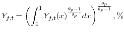
The economy's final good, $Y_{f,t}$ , is produced according to the Dixit-Stiglitz technology,

$\displaystyle Y_{f,t}=\left( \int_{0}^{1} Y_{f,t}(x)^{\frac{\theta_{p}-1}{\theta_{p}}% }dx\right) ^{\frac{\theta_{p}}{\theta_{p}-1}}, \%$

(1)

where the variable $Y_{f,t}(x)$ denotes the quantity of the

th differentiated goods used in production and $\theta_{p}$ is the constant elasticity of substitution between the differentiated production inputs.

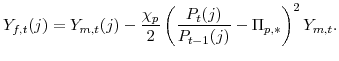
Final goods producers obtain their differentiated production inputs used in production from the economy's differentiated intermediate goods producers who supply an output $Y_{m,t}(x)$ . Not all of the differentiated output produced by the intermediate goods producers is realized as inputs into final goods production; some is absorbed in price formulation, following the adjustment cost model of Rotemberg (1982). Specifically, the relationship between $Y_{f,t}(j)$ and $Y_{m,t}(j)$ is given by,

$\displaystyle Y_{f,t}(j)=Y_{m,t}(j) -\frac{\chi_{p}}{2} \left( \frac{P_{t}(j)}{P_{t-1}(j)} -\Pi_{p,\ast} \right) ^{2}Y_{m,t}.%$

(2)

The second term in (2) denotes the cost of setting prices. This is quadratic in the difference between the actual change in price and steady-state change in price, $\Pi_{p,\ast}$ .

Our choice of quadratic adjustment costs for modeling nominal rigidities contrasts with that of many other recent studies, which rely instead on staggered price-and wage-setting in the spirit of Calvo (1983) and Taylor (1980). We prefer the quadratic adjustment cost approach over staggered price- and wage-setting because the latter imply heterogeneity among agents. Partly for this reason, models utilizing staggered price and wage setting typically assume that utility is separable between consumption and leisure, in which case perfect insurance among households against labor income risk eliminates heterogeneity of their spending decisions. By contrast, if wages are staggered and household utility is nonseparable, differences across households in labor supply (which will result due to differences in wages set) lead to differences across household in the marginal utility of consumption (and hence consumption), even if perfect insurance is able to equalize wealth across households. The quadratic adjustment cost model allows us to avoid heterogeneity across agents. In any case, the resulting price and wage inflation equations are very similar to those derived from Calvo-based setups as in Erceg, Henderson, and Levin (2000).

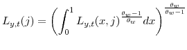
The differentiated intermediate goods, $Y_{m,t}(j)$ for $j \in[0,1]$ , are produced by combining each variety of the economy's differentiated labor inputs that are supplied to market activities (that is, $\{L_{y,t}(z)\}$ for $z \in[0,1]$ ). The composite bundle of labor, denoted $L_{y,t}$ , that obtains from this aggregation implies, given the current level of technology $A_{t}$ , the output of the differentiated goods, $Y_{m,t}$ . Specifically, production is given by,

$\displaystyle Y_{m,t}(j) = A_{t}L_{y,t}(j)$ where $\displaystyle L_{y,t}(j)=\left( \int_{0}^{1} L_{y,t}(x,j)^{\frac{\theta_{w}-1}{\theta_{w}}} dx \right) ^{\frac{\theta_{w}% }{\theta_{w}-1}}%$

(3)

and where $\theta_{w}$ is the constant elasticity of substitution between the differentiated labor inputs. The log-level of technology, $A_{t}$ , is modeled as a random walk

$\displaystyle \ln A_{t}= \ln A_{t-1} + \epsilon_{t},%$

(4)

where $\epsilon_{t}$ is an i.i.d. innovation. We abstract from trend growth in productivity. Throughout this paper, we restrict our analysis to permanent shocks to the level of technology.

2.2 Preferences

Households derive utility from their purchases of the consumption good $C_{t}$ and from their use of leisure time, equal to what remains of their time endowment $\bar{L}$ after $0 \leq L_{u,t}(i) \leq\bar L$ hours of labor are supplied to non-gratifying activities. We assume the household members live forever and there is no population growth. Its preferences exhibit an endogenous additive habit (assumed to equal a fraction $\eta\in[0,1]$ of its consumption last period) and are nonseparable between consumption and leisure.¹Specifically, preferences of household are given by

$\displaystyle E_{0}\frac{1}{1-\sigma}\sum_{t=0}^{\infty}\beta^{t} \left[ (C_{t}(i)-\eta C_{t-1}(i)) (\bar{L}-L_{u,t}(i))^{\zeta}\right] ^{1-\sigma},%$

(5)

where $\beta$ is the household's discount factor, and $\zeta$ is a measure of the utility of leisure. The economy's resource constraint implies that $\int_{0}^{1} C_{t}(x) dx \leq Y_{f,t}$ , where $Y_{f,t}$ denotes the output of the economy's final good.

Non-gratifying activities include supplying $L_{y,t}$ hours to the labor market and devoting time to setting wages. Consequently, we define $L_{u,t}(i)$ as

$\displaystyle L_{u,t}(i)=L_{y,t}(i) +\frac{\chi_{w}}{2} \left( \frac{W_{t}(i)}{W_{t-1}(i)} -\Pi_{w,\ast} \right) ^{2}L_{u,t}.%$

(6)

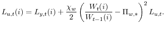
The second term in (6) denotes the cost of setting wages in terms of labor time and is analogous to the cost of setting prices.

2.3 Firms' optimization problems

The final goods producing firm, taking as given the prices set by each intermediate-good producer for their differentiated output, $\{P_{t}% (j)\}_{j=0}^{1}$ , chooses intermediate inputs, $\{Y_{f,t}(j)\}_{j=0}^{1}$ , so as to minimize the cost of producing its final output $Y_{f,t}$ , subject its production technology, given by equation (1). Specifically, the competitive firm in each sector solves

$\displaystyle \min_{\{Y_{f,t}(j) \}_{j=0}^{1} } \int_{0}^{1} P_{t}(x)Y_{f,t}(x)dx$ s.t. $\displaystyle Y_{f,t}\leq\left( \int_{0}^{1}Y_{f,t}(x) ^{\frac{\theta_{p}-1}% {\theta_{p}}}dx\right) ^{\frac{\theta_{p}}{\theta_{p}-1}}.%$

(7)

This problem implies a demand function for each of the economy's intermediate goods given by $Y_{f,t}(j) =\left( P_{t}(j)/P_{t}\right) ^{-\theta_{p}} Y_{f,t}$ , where the variable $P_{t}$ is the aggregate price level, defined by $P_{t}=(\int_{0}^{1}(P_{t}(x))^{1-\theta_{p}}dx)^{\frac{1}{1-\theta_{p}}}$ .

Each intermediate firm chooses the quantities of labor that it employ use for production and the price that it will set for its output. It is convenient to consider these two decisions as separate problems. In the first step of the problem firm , taking as given the wages $\{ W_{t}(i) \}_{i=0}^{1}$ set by each household for its variety of labor, chooses $\{ L_{y,t}(i,j)\}_{i=0}^{1}$ to minimize the cost of attaining the aggregate labor bundle $L_{y,t}(j)$ that it will ultimately need for production. Specifically, the materials firm solves:

$\displaystyle \min_{\{L_{y,t}(i,j) \}_{i=0}^{1} } \int_{0}^{1} \! W_{t}(x)L_{y,t}(x,j)dx$ s.t. $\displaystyle Y_{m,t}(j)\!\leq\! A_{t}\left( \int_{0}^{1} L_{y,t}% (x,j)^{\frac{\theta_{w}-1}{\theta_{w}}} dx \right) ^{\frac{\theta_{w}}% {\theta_{w}-1}}%$

(8)

This cost-minimization problem implies that the economy-wide demand for type

labor is $L_{y,t}(i)=\int_{0}^{1} L_{y,t}(i,x) dx =\left( W_{t}% (i)/W_{t}\right) ^{-\theta_{w}} \left( 1/A_{t}\right) \int_{0}^{1} Y_{m,t}(x)dx$ where $W_{t}$ denotes the aggregate wage, defined by $W_{t}=(\int_{0}^{1}(W_{t}(x))^{1-\theta_{w}}dx)^{\frac{1}{1-\theta_{w}}}$ . The marginal cost function of producing the intermediate goods is $MC_{t}(j)=W_{t}/A_{t}$ .

In setting its price, $P_{t}(j)$ , the intermediate good producing firm takes into account the demand schedule for its output that it faces from the final goods sectors and the fact--as summarized in equation (2)--that by resetting its price it reduces the amount of its output that it can sell to final goods producers. The intermediate-good producing firm , taking as given the marginal cost $MC_{t}(j)$ for producing $Y_{m,t}(j)$ , the aggregate price level $P_{t}$ , and aggregate final-goods demand $Y_{f,t}$ , chooses its price $P_{t}(j)$ to maximize the present discounted value of its profits subject to the cost of re-setting its price and the demand curve it faces for its differentiated output. Specifically, the firm solves,

	$\displaystyle \max_{\{P_{t}(j)\}_{t=0}^{\infty}} E_{0}\sum _{t=0}^{\infty}\beta^{t}\!\frac{\Lambda_{c,t}}{P_{t}} \left\{ (1+\varsigma _{\theta,p})P_{t}(j)Y_{f,t}(j)-MC_{t}(j)Y_{m,t}(j) \right\}$
	$\displaystyle$ subject to
	$\displaystyle Y_{f,t}(j)\!=\!Y_{m,t}(j) \!-\frac{\chi_{p}}{2} \left( \frac{P_{t}(j)}{P_{t-1}(j)} \!-\Pi_{p,\ast} \right) ^{2}\!\!Y_{m,t}$ and $\displaystyle Y_{f,t}(j) \!=\!\left( \frac{P_{t}(j)}{P_{t}}\right) ^{-\theta_{p}}\!\!Y_{f,t},%$	(9)

In (9) the discount factor that is relevant for discounting nominal revenues and costs between periods

and

is $E_{t} \beta^{j} \frac{\Lambda_{c,t+j}/P_{t+j}}{\Lambda_{c,t}/P_{t}}$ , where $\Lambda_{c,t}$ is the household's marginal utility of consumption in period

. The parameter $\varsigma_{\theta,p}$ is a subsidy that we assume equals $(\theta_{p}% -1)^{-1}$ ), which ensures that in the absence of nominal rigidities the model's equilibrium outcome is Pareto optimal.²

2.4 Households' optimization problem

The household taking as given the expected path of the gross nominal interest rate $R_{t}$ , the price level $P_{t}$ , the aggregate wage rate $W_{t}$ , its profits income, and its initial bond stock $B_{i,0}$ , chooses its consumption $C_{t} (i)$ and its wage $W_{t}(i)$ to maximize its utility subject to its budget constraint, the cost of re-setting its wage, and the demand curve it faces for its differentiated labor. Specifically, the household solves:

	$\displaystyle \max_{\left\{ C_{t}(i), W_{t}(i) \right\} _{t=0}^{\infty}} E_{0}\frac{1}{1-\sigma}\sum_{t=0}^{\infty}\beta^{t}\Xi_{c,t} \left[ (C_{t}(i)-\eta C_{t-1}(i)) (\bar{L}-L_{u,t}(i))^{\zeta}\right] ^{1-\sigma}$
	$\displaystyle$ subject to
	$\displaystyle E_{t}\left[ \beta\frac{\Lambda_{c,t+1}/P_{c,t+1}}{\Lambda _{c,t}/P_{c,t}} B_{t+1}(i)\right] \!=\!B_{t}(i)+(1+\varsigma_{\theta,w}% )W_{t}(i)L_{y,t}(i)+\mathit{Profits}_{t}(i)-P_{t}C_{t}(i),$
	$\displaystyle L_{y,t}(i)=L_{u,t}(i) -\frac{\chi_{w}}{2} \left( \frac{W_{t}% (i)}{W_{t-1}(i)} -\Pi_{w,\ast} \right) ^{2}L_{u,t}, \text{and}$
	$\displaystyle L_{y,t}(i)\!=\!\left( \!\frac{W_{t}(i)}{W_{t}}\!\right) ^{\!-\theta_{w}}\!\int_{0}^{1} \! L_{y,t}(i,j)dj.%$	(10)

The parameter $\varsigma_{\theta,w}$ in the household's budget constraint is a subsidy (equal to $(\theta_{w}-1)^{-1}$ ), which ensures that in the absence of nominal rigidities the model's equilibrium outcome is Pareto optimal. The variable ${B}_{t}(i)$ in the budget constraint is the state-contingent value, in terms of the numeraire, of household

's asset holdings at the beginning of period

. We assume that there exists a risk-free one-period bond, which pays one unit of the numeraire in each state, and denote its yield--that is, the gross nominal interest rate between periods

and

--by $R_{t}\equiv\left( E_{t}\beta\frac{\Lambda_{c,t+1}/P_{t+1}} {\Lambda _{c,t}/P_{t}}\right) ^{-1}$ . Profits in the budget constraint are those rebated from firms, which are ultimately owned by households.

2.5 Steady-state and natural rate variables

The non-stochastic steady state is summarized by the steady-state levels of the real interest rate and hours. The steady-state one-period real interest rate is given by:

$\displaystyle R_{\ast} = \beta^{-1}.$

(11)

The steady-state level of hours is given by:

$\displaystyle L_{\ast} = \frac{\bar{L}} {1+\frac{1-\eta}{1-\beta\eta} \zeta}%$

(12)

Given the assumed non-stationarity of the level of technology, in the following we work with normalized variables, where we normalize the levels of consumption and output by the current level of technology. The normalized steady-state levels of consumption and output therefore equal the steady-state level of hours.

The model has a counterpart in which all nominal rigidities are absent, that is, prices and wages are fully flexible. In this model the cost minimization problems faced by the final goods producing firm and the intermediate goods producing firms continue to be given by equations (7) and (8). The intermediate goods producing firms' profit maximization problem is similar to equation (9) but with the price adjustment cost parameter $\chi_{p}$ set to zero. Likewise the households' utility maximization problem is given by equation (10) but with the wage adjustment cost parameter $\chi_{w}$ set to zero. We refer to the level of output and real one-period interest rate in this equilibrium as the natural rate of output, $\widetilde{Y}_{t}$ , and interest, $\widetilde{R}_{t}%$ . We also define log deviations of these variables from their steady-state values, $\tilde{y}_{t}\equiv\log\widetilde{Y}_{t}-\log Y_{\ast}$ and $\tilde{r}_{t}\equiv\log\widetilde{R}_{t}-\log R_{\ast}$ . These natural rates are functions of our model's structural shocks and are derived in Appendix A.

2.6 Monetary authority

In the model with nominal rigidities we assume that the central bank uses the short-term interest rate as its instrument, as discussed in section 4.

2.7 Equilibrium

Our complete model consists of the first-order conditions (derived in Appendix A) describing firms' optimal choice of prices and households' optimal choices of consumption and wages, the production technology (3), the monetary policy rule, the market clearing conditions $Y_{t}(j)=\int_{0}^{1} C_{j,t}(i) di \forall j$ and $L_{t}(i)=\int_{0}^{1} L_{i,t}(j) dj \forall i$ , and the law of motion for aggregate technology (4). We now turn to the parametrization of our model.

3 Estimation

In order to analyze optimal Bayesian monetary policy under parameter uncertainty, we need a posterior distribution of the model parameters. One approach to obtaining a posterior distribution, consistent with the Bayesian approach to decision-making assumed for the policymaker, is to estimate the model using Bayesian methods, as is done in LOWW. This approach necessitates making specific assumptions regarding the prior joint distribution of the model parameters. Because we want to avoid having the choice of the prior distribution overly influence our results, we instead follow a limited-information approach to estimating the posterior distribution of the model parameters.³ In particular, we estimate several of the structural parameters of our model using a minimum distance estimator based on impulse responses to monetary policy and technology shocks.

Specifically, we estimate a VAR on quarterly U.S. data using empirical counterparts to the theoretical variables in our model, and identify two of the model's structural shocks using identifying assumptions that are motivated by our theoretical model. We then choose model parameters to match as closely as possible the impulse responses to these two shocks implied by the model to those implied by an structural VAR.⁴ In this section we first describe the VAR and the identification of the two shocks, and then discuss our parameter estimates.

3.1 VAR specification and identification

The specification of our VAR is determined by the model developed in the previous section and our identification strategy for the structural shocks. Concerning the latter, we follow Galí (1999) and assume that the technology shock is the only shock that has a permanent effect on the level of output per hour. The monetary shock is identified by a standard restriction on contemporaneous responses. Our model and identifying assumptions combined suggest the inclusion of five variables in the VAR: the first difference of log output per hour, price inflation (the first difference of the log of the GDP deflator), the log labor share, the first difference of log hours per person, and the nominal funds rate. Output per hour, the labor share, and hours are the Bureau of Labor Statistics' (BLS) measures for the nonfarm business sector, where the labor share is computed as output per hour times the deflator for nonfarm business output divided by compensation per hour.⁵ Population is the civilian population age 16 and over. Letting $Y_{t}$ denote the vector of variables in the VAR, we view the data in the VAR as corresponding, up to constants, to the model variables

$\displaystyle Y_{t}=[\Delta(y_{t}-l_{t}), \pi_{t}, y_{t}-l_{t}-w_{t}, \Delta l_{t}, r_{t}]^{\prime}%$

(13)

where lower case letters denote logs of the model variables.⁶ We estimate the VAR over the sample 1966q2 to 2006q2, including four lags of each variable. Details of the implementation of the identification scheme are provided in Appendix B.

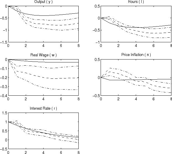
The dashed lines in the panels of Figure 1 show the impulse responses to a permanent one percent increase in the level of technology. The dashed-dotted lines present one-standard deviation bands around the impulse responses, computed by bootstrap methods.⁷ Upon impact, output immediately rises about half-way to its new steady-state level, whereas hours worked decline by about 1/4 percent. Over the following eight quarters, output completes its adjustment while hours worked return to their original level. Interestingly, the response of inflation to a technology shock suggests only a limited role for price stickiness, with inflation declining upon impact by almost a percentage point. Wage rigidity, by contrast, seems to be more important, as the initial response of the real wage is driven by the initial price response, not nominal wage adjustment. The real wage completes its adjustment over the following two quarters. The estimated response of monetary policy is to accommodate the increase in output by keeping the real funds rate on balance unchanged.

Figure 2 shows the impulse responses of the variables to a one percentage point positive funds rate shock. The estimated responses of output, the real wage, and inflation to a funds rate shock are consistent with many studies on the effects of monetary policy. Output falls within three quarters by about 3/4 percent in response to one percentage point increase in the funds rate that takes eight quarters to die out. Hours decline closely in line with output, and the real wage falls. The response of inflation exhibits a price puzzle that lasts for two quarters; thereafter, inflation declines for six quarters, to about 0.3 percent below its original level. The responses to a funds rate shock are more precisely estimated than the responses to the technology shock.

3.2 Model parameter estimates

With the VAR impulse responses to a funds rate shock and a technology shock in hand, we proceed to estimate the structural and monetary policy parameters of our model. First, we calibrate four model parameters that have little effect on the dynamic responses to shocks. We set the discount factor, $\beta= 0.9924$ , which corresponds to discounting the future at a 3 percent annual rate. We normalize the time endowment to unity. We set the steady-state rates of price and wage inflation to zero. Finally, we set both aggregation parameters $\theta_{w}$ and $\theta_{p}$ to 6, following LOWW (2005).

The remaining parameters are estimated by minimizing the squared deviations of the responses of the five variables $[y_{t}, \pi_{t}, w_{t}, l_{t}% , r_{t}]$ implied by our model from their VAR counterparts. The IRFs of these five variables in quarters 0 through 8 following a technology shock in quarter 0, and in quarters 1 through 8 following a funds rate shock (the response in the impact quarter being constrained by the identifying assumption) provide a total of 85 moments to match. These moments are weighted inversely proportional to the standard error around the VAR responses, as in Christiano et al. (2005). This has the effect of placing more weight on matching the impulse responses to the monetary shock, which, as noted before, are estimated with greater precision than the impulse responses to the technology shock.

For purposes of model estimation, we assume that monetary policy is set according to a simply policy rule in which the interest rate depends on the lagged interest rate and the current inflation rate only

$\displaystyle r_{t} = \phi_{r} r_{t-1} + (1-\phi_{r})\phi_{\pi}\pi_{p,t} + \epsilon_{r,t},$

where $\epsilon_{r,t}$ is an i.i.d. monetary policy shock.⁸ Note that we have suppressed the constant that incorporates the steady-state levels of the interest and inflation rate.

In addition, because the parameters $\theta_{w}$ and $\chi_{w}$ appear only as a ratio in the linearized version of the model (see Appendix A), they are not separately identified; the same is the case for the parameters $\theta_{p}$ and $\chi_{p}$ . We therefore estimate the ratios $\kappa_{w}=(\theta _{w}-1)(1+\varsigma_{\theta,w})/(\chi_{w}\Pi_{w,\ast}^{2})=\theta_{w}% /(\chi_{w}\Pi_{w,\ast}^{2})$ and $\kappa_{p}=(\theta_{p}-1)(1+\varsigma _{\theta,p})/(\chi_{p}\Pi_{p,\ast}^{2})=\theta_{p}/(\chi_{p}\Pi_{p,\ast}^{2}% )$ . Note that $\kappa_{w}$ and $\kappa_{p}$ are equal to the coefficients on the driving process in the wage and price Phillips curves, respectively. In the end, we estimated seven free parameters: $\{ \sigma, \zeta, \eta, \kappa_{w}, \kappa_{p}, \phi_{r}, \phi_{\pi} \}$ .

The estimated parameters and associated standard errors are shown in the first two columns of Table 1. The correlation coefficients of the structural parameter estimates are shown in the final five columns of the table. The covariance matrix of the estimates is computed using the Jacobian matrix from the numerical optimization routine and the empirical estimate of the covariance matrix of the impulse responses from the bootstrap. The estimates of the structural parameters are all statistically significant, with the preference parameters, especially $\sigma$ and $\zeta$ , relatively imprecisely estimated, while those associated with wage and price adjustment costs are estimated with a great deal of precision.

Table 1: Parameter Estimates
Model Parameter	Point Estimate	Standard Error	Corr. $\sigma$	Corr $\eta$	Corr. $\zeta$	Corr. $\kappa_{w}$	Corr. $\kappa_{p}$
$\sigma$	5.365	2.372	1.000	-0.996	-0.995	-0.960	-0.495
$\eta$	0.389	0.094		1.000	0.990	0.947	0.491
$\zeta$	1.186	0.386			1.00	0.971	0.478
$\kappa_{w}$	0.004	0.001				1.000	0.436
$\kappa_{p}$	0.041	0.001					1.000
$\phi_{r}$	0.809	0.001
$\phi_{\pi}$	1.004	0.027

As discussed before, one feature of both sets of impulse responses is that real output and hours adjust gradually in response to the shocks. In the case of a permanent technology shock, Rotemberg and Woodford (1996) demonstrated that DSGE models without intrinsic inertia will not display such hump-shaped patterns; instead, these variables jump on impact and adjust monotonically to their new steady-state values. We therefore find a significant role for habit persistence. Our estimate of the habit parameter $\eta$ is somewhat smaller than those estimated by Fuhrer (2000), Smets and Wouters (2003) and Christiano et al (2005), but slightly larger than that estimated by LOWW (2005). The estimate of $\sigma$ is higher than typical estimates based on macroeconomic data, but this estimate is very imprecise.

As noted before, the VAR responses of real wages and inflation differ substantially depending on the source of the shock: rapid responses to technology shocks, and sluggish ones to funds rate shocks. This is a feature that our price and wage specification cannot deliver. Our estimates of $\kappa_{w}$ and $\kappa_{p}$ imply that wages are very slow to adjust, but prices adjust relatively rapidly to fundamentals. The evidence for relatively flexible prices comes from the IRFs to the technology shock; indeed, the IRFs to monetary policy shocks alone suggest very gradual price adjustment, consistent with the findings of Christiano et al (2005). Despite the greater weight placed on matching the more tightly estimated responses of inflation and real wage to the funds rate shock, our model does better at matching the responses to a technology shock, as shown by the solid lines in figures 1 and 2. Our estimates of the parameters of the monetary policy rule, $\phi_{r}$ and $\phi_{\pi}$ , are broadly consistent with the findings of many other studies that estimate monetary policy reaction functions, such as that of Clarida, Galí, and Gertler (2000).

4 Welfare and Optimal Monetary Policy

In this section we compute the optimal policy response to a technology shock assuming all model parameters are known. We assume that the central bank objective is to maximize the unconditional expectation of the welfare of the representative household. We further assume that the central bank has the ability to commit to future policy actions; that is, we examine optimal policy under commitment, as opposed to discretion. We consider only policies that yield a unique rational expectations equilibrium.

By focusing only on technology shocks, we are arguably examining only a relatively small source of aggregate fluctuations in output and wage and price inflation and hence welfare losses. For example, LOWW (2005), using a medium-scale DSGE model, find that other shocks, especially those to price and wage markups, have much larger effects on welfare than technology shocks. In order to conduct welfare-based monetary policy analysis incorporating other sources of fluctuations, we would need to take a stand on the precise source and nature (i.e., distortionary vs. fundamental) of the other shocks to the economy, as discussed in LOWW (2005). This issue remains controversial and would take us afield of the primary purpose of the paper, and we therefore leave it to further research. Nonetheless, we recognize that by abstracting from other shocks, our quantitative results regarding welfare costs under alternative policies likely dramatically understate those that would obtain if we included a full specification of all shocks that impact the economy.

4.1 Approximating Household Welfare

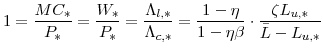
As is now standard in the literature, we approximate household utility with a second-order Taylor expansion around the deterministic steady state. We denote steady-state values with an asterisk subscript. As shown in Appendix D, the second-order approximation of the period utility function depends on the squared output gap (the log difference between output and its natural rate, that is $x_{t}=y_{t}-y^{n}_{t}$ ), the squared quasi-difference of the output gap, the cross-product of the output gap and its quasi-difference, and the squared price and wage inflation rates. As shown in the appendix, in the linearized model, the natural rate of output, $y^{n}_{t}%$ , is a function of leads and lags of the technology shock.

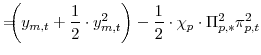
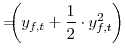
After numerous manipulations, the second-order approximation to period utility can be written as

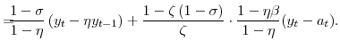
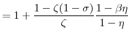
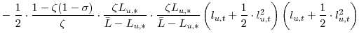
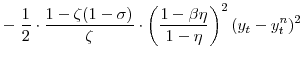
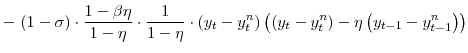
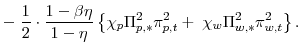
$\displaystyle \frac{1}{1-\sigma}\left[ \left( C_{t}-\eta C_{t-1}\right) \left( \bar {L}-L_{u,t}\right) ^{\zeta}\right] ^{1-\sigma} =-\mathcal{L}+\mathrm{T.I.P.}, \mathrm{where} \mathcal{L}\equiv\mathcal{L}_{x}+\mathcal{L}_{p}% +\mathcal{L}_{w}$

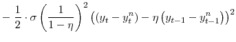
and where T.I.P refers to terms that are independent of monetary policy, which we ignore in our welfare calculations. The terms $\mathcal{L}_{x}$ , $\mathcal{L}_{p}$ , and $\mathcal{L}_{w}$ defined as

$\displaystyle \mathcal{L}_{x} \!\!\!\!$	$\displaystyle =\!\!\!\! \left[ \left( C_{\ast}\!-\!\eta C_{\ast }\right) \left( \bar{L}\!-\!L_{u,\ast}\right) ^{\zeta}\right] ^{1-\sigma}\! \left[ \frac{1}{2} \cdot\frac{1\!-\!\zeta(1\!-\!\sigma)}{\zeta} \cdot\left( \frac{1\!-\!\beta\eta}{1\!-\!\eta}\right) ^{2}\!x_{t}^{2} \right. +\frac {1}{2} \cdot\frac{\sigma}{(1\!-\!\eta)^{2}} \cdot\left( x_{t}\!-\!\eta x_{t-1}\right) ^{2}$
	$\displaystyle \left. + (1\!-\!\sigma)\cdot\frac{1\!-\!\beta\eta}{(1\!-\!\eta)^{2}}\;x_{t} \left( x_{t}\!-\!\eta x_{t-1} \right) \right] \!,$
$\displaystyle \mathcal{L}_{p} \!\!\!\!$	$\displaystyle =\!\!\!\! \left[ \left( C_{\ast}\!-\!\eta C_{\ast }\right) \left( \bar{L}\!-\!L_{u,\ast}\right) ^{\zeta}\right] ^{1-\sigma}\! \left[ \frac{1}{2} \cdot\frac{1-\beta\eta}{1-\eta} \cdot\frac{\theta_{p} \Pi_{p,\ast}}{\kappa_{p}} \cdot\pi_{p,t}^{2}\right] ,\; \mathrm{and}%$
$\displaystyle \mathcal{L}_{w} \!\!\!\!$	$\displaystyle =\!\!\!\! \left[ \left( C_{\ast}\!-\!\eta C_{\ast }\right) \left( \bar{L}\!-\!L_{u,\ast}\right) ^{\zeta}\right] ^{1-\sigma}\! \left[ \frac{1}{2} \cdot\frac{1-\beta\eta}{1-\eta} \cdot\frac{\theta_{w} \Pi_{w,\ast}}{\kappa_{w}} \cdot\pi_{w,t}^{2}\right] .$

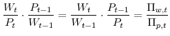
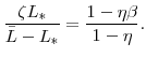
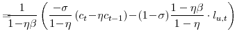
The three terms in $\mathcal{L}_{x}$ correspond to the period welfare costs associated with output deviating from its natural rate. Owing to the presence of habit formation, both the level of the output gap and its quasi-difference affect welfare. Note that all three preference parameters enter in the coefficients of the welfare loss for these terms. The terms in $\mathcal{L}% _{p}$ and $\mathcal{L}_{w}$ corresponds to the welfare loss associated with adjustment costs in changing prices and wages. The coefficients in these terms depend primarily on the parameters associated with nominal rigidities. Importantly, the welfare costs of sticky prices and wages are inversely related to the price and wage sensitivity parameters, $\kappa_{p}$ and $\kappa_{w}$ , respectively. The more flexible are prices, the smaller are the welfare costs associated with a given magnitude of inflation fluctuations, and similarly for wages.⁹ In the following, we report the period welfare loss abstracting from the terms of independent of policy, $\mathcal{L}$ , as well as the three components of the loss, $\mathcal{L}_{x}$ , $\mathcal{L}_{p},$ and $\mathcal{L}_{w}$ described above.

Table 2 reports the implied relative weights on the terms related to the output gap, wage inflation, and price inflation.¹⁰ The first row reports the sum of the weights on the three terms in the loss associated with the output gap and its quasi-difference.¹¹ For this table, we have normalized the values of the weights by the weight on price inflation evaluated at the parameter point estimates. The first column reports the weights based on the parameter point estimates. The second column reports the mean values of the weights based on the estimated distribution of the parameter values, approximated using 1000 draws from the normal distribution with the estimated covariance for the parameter estimates, where we truncate the parameter values at the lower ends of their distributions as follows: $\sigma$ at 0.5, $\zeta$ at 0.1, and $\eta$ at 0. The third column reports the corresponding standard deviations of the weights. The final three columns report the cross-correlation of the weights.

Table 2: Relative Weights in Central Bank Loss
Weight in Loss	Point Estimate	Mean Value	Standard Deviation	Corr. $\omega_{x}$	Corr. $\omega_{w}$	Corr. $\omega_{p}$
$\omega_{x}$	0.14	0.38	0.49	1.000	0.996	0.996
$\omega_{p}$	1.00	2.31	2.86		1.000	0.989
$\omega_{w}$	10.56	29.09	38.11			1.000

Based on the point estimates, the variance in wage inflation gets a weight of over 10 times that of price inflation in the welfare loss owing to the estimated value of $\kappa_{w}$ being one tenth as large as that for $\kappa_{p}$ . The weights on the variances of the output gap and the quasi-difference of the output gap are somewhat smaller than that of inflation, but are somewhat higher than typically seen in the literature owing to our relatively high estimate of $\sigma$ . The mean values of the weights exhibit the same pattern, but are between two and three times larger than those based on the point estimates, reflecting the fact that the weights depend in part on the inverse of some parameter values.

The relative weights are highly positively correlated, reflecting the fact that the structural parameter estimates are highly correlated with one another and that each component of the welfare loss depends on the steady-state level of utility. As seen in Table 1, the estimates of $\sigma$ and $\zeta$ are highly negatively correlated, which is not surprising given that these two parameters enter multiplicatively in the utility of leisure. More interestingly, the estimate of $\sigma$ is negatively correlated with the estimated values of $\kappa_{p}$ and $\kappa_{w}$ , implying that a large weight on output gap terms is associated with large weights on price and wage inflation terms and vice versa.

4.2 Optimal Monetary Policy with No Uncertainty

To compute the optimal certainty equivalent policy for a given set of parameter values, we maximize the quadratic approximation of welfare subject to the constraints implied by the linearized model. Throughout, in computing the welfare loss we assume a discount rate arbitrarily close to zero, so that we are maximizing the unconditional measure of welfare. We compute the fully optimal policy using Lagrangian methods as described in Finan and Tetlow (1999). We assume that the technology shock is the only stochastic element in the model and calibrate the standard deviation of its innovations to equal 0.64 percentage point. This value is slightly larger than the corresponding estimate in LOWW (2005).

The results under the fully optimal policy are shown in the first column of Table 3. The middle portion of the table shows the welfare loss and the breakdown into its component parts (the components add to the total welfare loss, subject to rounding).¹² Note that we do not normalize the welfare loss in this table or in those that follow. The lower part of the table reports the resulting unconditional standard deviations of output gap, price and wage inflation rates, and the nominal interest rate. The remaining entries in the table are discussed below.

Table 3: Performance of Alternative Monetary Policies without Uncertainty
	Optimal Policy	Policy Rule Coefficients (1)	Policy Rule Coefficients (2)	Policy Rule Coefficients (3)	Policy Rule Coefficients (4)
$r^{n}$		1.00	1.00
		1000.00
					1.93
$\pi_{p}$		0.10	0.00	94.94	0.00
$\pi_{w}$			2.50	1000.00
Welfare Losses: $\mathcal{L}$	1.758	1.760	1.758	1.760	1.760
Welfare Losses: $\mathcal{L}_{x}$	0.002	0.000	0.001	0.003	0.001
Welfare Losses: $\mathcal{L}_{p}$	1.618	1.608	1.622	1.612	1.605
Welfare Losses: $\mathcal{L}_{w}$	0.138	0.152	0.135	0.145	0.154
Standard Deviations:	.02	.00	.02	.02	.01
Standard Deviations: $\pi_{p}$	.19	.19	.19	.19	.19
Standard Deviations: $\pi_{w}$	.02	.02	.02	.02	.02
Standard Deviations:	.87	.88	.88	.80	.82

Under the fully optimal monetary policy, output gap and wage inflation variability are reduced to nearly zero, while some price inflation variability remains. In terms of the annualized rate, the standard deviation of price inflation is 0.8 percentage points, about 10 times greater than that of wage inflation. Note that this policy induces considerable interest rate variability in response to a single source of shocks, with the standard deviation of the nominal interest rate 3.6 percentage points on an annualized basis.¹³ Under the optimal policy, variability in price inflation accounts for most of the welfare loss.

4.3 Implementable Monetary Policy Rules

The fully optimal monetary policy can be implemented in a number of equivalent ways if all model parameters are known with certainty. In the presence of parameter uncertainty, we need to restrict ourselves to representations of monetary policy that are constrained by the information set that the policymaker possesses. For this purpose, we choose to study monetary policies in terms of feedback or "instrument" rules where the short-term interest rate is determined by a small number of observable variables and the coefficients of the policy rule are chosen to minimize the welfare loss. We consider four different specifications of monetary policy, each of which yields welfare very close to the fully optimal policy when all parameters are known.

The general specification is given by a Taylor-type monetary policy rule where the nominal interest rate is determined by the central bank estimate of the natural rate of interest, $r^{n}_{t}$ , the central bank estimate of the output gap, $x_{t}$ , the level of hours, $l_{t}$ , and the rates of price and wage inflation:

$\displaystyle r_{t} = \pi_{p,t} + \phi_{r^{n}} r^{n}_{t} + \phi_{x} \; x_{t} + \phi_{l} \; l_{t} + \phi_{p} \; \pi_{p,t} + \phi_{w} \; \pi_{w,t}.$

(14)

Note that we have included the price inflation rate as the first term of the equation, implying that the policy yields a unique rational expectations equilibrium as long as one of the other coefficients (on price inflation, wage inflation, the output gap, or the level of hours) is strictly positive. The response to hours is assumed to be to the level of hours, not the hours "gap." With known parameters, the central bank estimates of the natural rates equal their respective true values.

We start by considering a textbook Taylor rule with a unit response to the natural rate of interest and a free coefficients on the rates of price inflation and the output gap. We optimized the coefficients of this rule to maximize unconditional welfare of the representative household using a numerical hill-climber routine, as described in Levin, Wieland, and Williams (1999). Throughout the following, we restrict policy rule coefficients to be non-negative and to not exceed an upper bound of 1000.¹⁴ The results for the optimized Taylor rule are given in the second column in the table. The optimized Taylor rule has a small coefficient on the price inflation rate and the maximal allowable coefficient on the output gap. This rule strives to keep the output gap at zero. The resulting outcome yields a welfare loss nearly identical to the fully optimal policy, with very slightly too much wage inflation variability.

We next consider a variant of the Taylor rule where policy responds to the rate of wage inflation instead of the output gap. This rule features a zero optimal response to price inflation and a moderate response to wage inflation. The resulting outcomes and corresponding welfare are virtually identical to those under the fully optimal policy.

Finally, we consider two alternative specifications of the monetary policy rule that do not depend on estimates of the natural rates of output or interest. Interestingly, in both cases, the optimized versions of these rules nearly match the outcomes under the fully optimal policy. First, we consider a rule that does not respond to the natural rate of interest (except for its long-run mean) or any measure of economic activity, but instead responds only to price and wage inflation. The optimized parameterization of this rule features huge responses to price and wage inflation with the response to wage inflation about 10 times larger than that to price inflation. Second, we consider a rule that responds to price inflation and the log-level of hours. For this rule, the optimized response to price inflation is zero and that to hours is about 2.

5 Monetary Policy under Parameter Uncertainty

In this section, we analyze the performance and robustness of various monetary policies under parameter uncertainty. We assume that the central bank knows the true model and that the model is estimated using a consistent estimator and that the central bank is certain that the model and the estimation methodology are correct.¹⁵ The only form of uncertainty facing the policymaker is uncertainty regarding model parameters owing to sample variation. We abstract from learning and assume that the policymaker's uncertainty does not change over time. We assume that private agents know everything, including the central bank's parameter estimates. For a given policy rule, expected welfare is computed by numerically integrating over the distribution of the five estimated structural parameters as measured by the estimated covariance matrix. Note that in these calculations, we fully take into account the effects of parameter values on the parameters of the loss function as in Levin and Williams (2005).

5.1 Natural Rate Uncertainty

Before proceeding with the analysis of policy rules, we first provide some summary measures of the degree of uncertainty regarding the natural rates of hours, output, and interest owing to parameter uncertainty. In this model, the responses of the natural rates to a technology shock depend on three parameters describing household preferences: $\sigma$ , $\eta$ , and $\zeta$ . Throughout the following, we assume that the distribution of model parameters is jointly normal distributed with mean zero and covariance given by the estimated covariance matrix. In the following, we approximate this distribution with a large number of draws from the estimated covariance matrix, truncated as described in section 3.

In general, parameter uncertainty implies uncertainty both about the steady-state values of natural rates as well as their movements over time. In the stylized model that we study here, however, the steady-state natural rate of interest depends only on the household's discount rate, which is assumed to be known by the policymaker. Therefore, uncertainty about the natural rate of interest is limited to its deviations from steady-state. The steady-state level of hours depends on estimated structural parameters and the value of the time endowment. Our estimation methodology does not use information on levels of variables, so we do not have an empirical measure of uncertainty regarding the time endowment. For simplicity, we assume that the policymaker, by observing a long time series on hours, is able to estimate the mean level of hours precisely. We assume that policymaker has no independent knowledge of the time endowment, so perfect knowledge of the mean level of hours has no implications for uncertainty about other preference parameters. We note that under less restrictive assumptions, there exist tight links between estimated structural parameters and steady-state values, which affect both model estimation and the analysis of parameter uncertainty.¹⁶

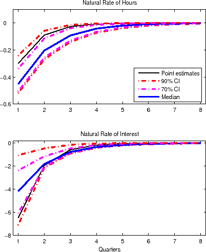
Parameter uncertainty implies considerable uncertainty regarding the responses of natural rates to technology shocks. The thin solid line in the upper panel of Figure 3 plots the impulse response of the log of the natural rate of hours to a one percentage point positive permanent technology shock based on the point estimates of the model parameters. (Note that the log of the natural rate of hours equals the log of the natural rate of output minus the log of TFP.) The thick solid line shows the median response calculated from impulse responses corresponding to 10,000 draws from the estimated parameter distribution. The dashed and dashed-dotted lines show the boundaries of the 70 and 90 percent confidence bands of the impulse responses, respectively. The lower panel of the figure shows the corresponding outcomes for the natural rate of interest measured at an annualized rate. Note that the model implies that there is no uncertainty about the long-run effects of technology shocks on the natural rates of hours and interest, both of which eventually return to their respective steady state values.

Natural rate misperceptions owing to parameter uncertainty are sizable and persistent. We measure natural rate misperceptions as the difference between the level of the natural rate implied by the model's true parameter values and the level implied by the point estimates of the model parameters.¹⁷ To compute unconditional moments in our model, we calibrate the standard deviation of innovations to technology to equal 0.64 percentage point, equal to the sample average of the identified shocks from our VAR. The resulting unconditional standard deviation of the difference between the true natural rate of output and the central bank's estimate (based on the model with the parameter point estimates) is 0.32 percentage point. The first-order autocorrelation of this difference is 0.86. The unconditional standard deviation of the difference between the natural rate of interest and the central bank's estimate is 3.15 percentage points (measured at an annual rate), with a first-order autocorrelation of this difference equal to 0.50.

5.2 Optimal Monetary Policy under Parameter Uncertainty

In order to provide a benchmark for policies under uncertainty, we first compute the optimal outcome if the policymaker knew all the parameter values and followed the fully optimal policy in each case. We average the outcomes and losses over 1000 draws of the parameters and report the results in the first column of Table 4. Of course, given that the parameters are uncertain, this outcome is not obtainable in practice, but provides a benchmark against which we can measure the costs associated with parameter uncertainty. As can be seen from comparing the first columns of Tables 3 and 4, the mean welfare loss under the first-best optimal policy is considerably larger than that computed at the parameter point estimates. This reflects the fact that the mean weights in the welfare loss are higher than the weights evaluated at the point estimates. Indeed, under the first-best optimal policy, the variability of the objective variables is about the same as for the case of the parameter point estimates.

Table 4: Performance of Alternative Monetary Policies with Parameter Uncertainty
	Optimal Policy	Policy Rule Coefficients (1)	Policy Rule Coefficients (2)	Policy Rule Coefficients (3)	Policy Rule Coefficients (4)	Policy Rule Coefficients (5)
$\tilde r^{n}$		1.00	1.00			0.83
$\tilde x$		0.83				1.80
					3.69	2.99
$\pi_{p}$		0.00	75.78	82.58	0.00	14.40
$\pi_{w}$			1000.00	1000.00		210.00
Welfare Losses: $\mathcal{L}$	4.056	4.112	4.082	4.094	4.089	4.065
Welfare Losses: $\mathcal{L}_{x}$	0.003	0.050	0.028	0.036	0.026	0.012
Welfare Losses: $\mathcal{L}_{p}$	3.775	3.734	3.783	3.760	3.748	3.786
Welfare Losses: $\mathcal{L}_{w}$	0.278	0.328	0.272	0.298	0.315	0.267
Standard Deviations:	.02	.08	.07	.07	.08	.04
Standard Deviations: $\pi_{p}$	.19	.19	.19	.19	.19	.19
Standard Deviations: $\pi_{w}$	.02	.02	.01	.02	.02	.02
Standard Deviations:	.88	.87	.82	.76	1.08	.99

We now examine the characteristics and performance of the implementable monetary policy rules introduced in the previous section, but now we reoptimize the coefficients to minimize the expected welfare loss under parameter uncertainty. In implementing these rules, we assume that the central bank's estimates of the natural rates of output and interest are computed using the point estimates of the model parameters, but that the actual model parameters and therefore natural rates differ from the values assumed by the policymaker. The central bank is assumed to observe the technology shocks without error since these do not depend on model parameters.

Relative to the case of no parameter uncertainty, the optimized standard Taylor rule under parameter uncertainty responds far less aggressively to the estimate of the output gap. Recall that in the case of known parameters the optimized response to the output gap is 1000 (the imposed upper bound). In contrast, under parameter uncertainty, the optimal response coefficient is less than unity. This reduction in the response to the output gap is a consequence of the mismeasurement of the natural rate of output. Indeed, if the central bank faced parameter uncertainty but somehow knew the true values of the natural rates, the optimized Taylor rule would have the same huge response to the output gap that obtains absent parameter uncertainty and the mean welfare loss would be nearly the same as the benchmark first-best outcome.¹⁸ Thus, if natural rates were known, parameter uncertainty would be of little consequence for monetary policy or the mean welfare loss. But, in the presence of natural rate uncertainty, a large response to the output gap generates correspondingly large policy errors. In order to minimize this source of undesired fluctuations, the optimized rule responds much more modestly to the perceived output gap. As a result, this policy does not stabilize the output gap as well as the first-best policy.

The alternative policy that responds to the natural rate of interest and the rates of wage and price inflation yields a loss nearly identical to the first-best. As in the case of no parameter uncertainty, this policy rule responds extremely aggressively to the wage inflation rate and less so to the price inflation rate. The ratio of the response to wages to prices is slightly larger under parameter uncertainty than with no uncertainty. Interestingly, this policy does a better job on average of stabilizing the output gap than the optimized Taylor rule that responds directly to he output gap.

Optimized policy rules that respond to wage and price inflation and the natural rate of interest are very effective at minimizing the welfare loss under parameter uncertainty. Evidently, responding to aggressively to the wage inflation rate substitutes for responding to the output gap in this model, at least when evaluated using responses to technology shocks. Eliminating the response to the natural rate of interest causes a small deterioration in performance, as seen by the third alternative policy rule.

The fourth alternative optimized policy rule, that responds to only the level of hours (with the optimized response to price inflation of zero), performs nearly as well as any of the other rules, including those that respond to estimates of the natural rates. Given the emphasis on these natural rate concepts in the literature, this result that natural rates are nearly superfluous for optimal policy under parameter uncertainty may appear somewhat surprising. But, in an environment where natural rates are uncertain, their usefulness as indicators for monetary policy is reduced. Indeed, "imperfect" indicators such as the level of hours can perform as well or better than natural rate-based indicators like the output gap.

Finally, we examine optimized monetary policy rules that combined features of the simple policy rules considered above by responding to all five variables: the natural rate of interest, the output gap, the level of hours, and the rates of price and wage inflation. The results are reported in the final column of Table 4. The optimized version of this rule yields a welfare loss only slightly larger than the artificial first-best benchmark. The policy features a very aggressive response to wage inflation and a moderate response to the level of hours and relatively muted responses to the natural rate of interest and the output gap.

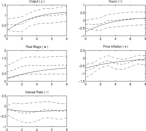
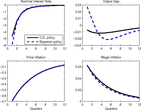
The optimal policy taking account of parameter uncertainty yields a larger response of the interest rate to a technology shock than the optimal policy under known parameters (the certainty equivalent policy). Figure 4 shows the impulse responses to a one percentage point positive technology shock under the optimal policy assuming known parameters (the solid lines) and the optimal "Bayesian" policy that takes account of parameter uncertainty by minimizing the mean welfare loss. In both cases, the impulse responses are computed using the parameter point estimates. Under the optimal Bayesian policy, the lower initial interest rate causes the output gap to rise above zero, which then gap swings back below zero where it remains for several years. Compared to the certainty-equivalent policy, the Bayesian policy generates greater variability in the output gap, but smaller variability in the wage inflation rate. The variability of the rate of price inflation is nearly identical under the two policies.

6 Conclusions

Three crucial factors determine the design of optimal monetary policy: the dynamics of the economy, the natural rates of output and interest, and the weights in the central bank objective function. Traditional analysis of monetary policy under uncertainty has treated these three factors as being independent and studied them separately. But, modern micro-founded models imply that the structural parameters describing preferences and technology jointly determine all three factors and that parameter uncertainty affects all three factors together. This paper has shown in an estimated micro-founded macroeconomic model that uncertainty about the natural rates of interest and output owing to parameter uncertainty has significant implication for the design of optimal monetary policy in the face of parameter uncertainty. In particular, we find that parameter uncertainty implies that monetary policy should be re-oriented away from directly responding to measures of the output gap, which are based on natural-rate estimates that are likely measured with error, and toward responding to variables that are not contaminated by such mismeasurement.

This paper has taken a first step at analyzing the implications of uncertainty about natural rates for monetary policy aimed at maximizing household welfare. In order to make the analysis as tractable as possible, we have used a small-scale stylized model and limited our analysis to parameter and natural rate uncertainty that results from sampling variation. As a result, the analysis has likely understated the true degree of uncertainty that central banks face regarding the economy and natural rates. The analysis can be extended to include additional features of the economic landscape and associated uncertainty, including a richer description of the macroeconomy, a wider set of sources of aggregate fluctuations, and uncertainty regarding the structure of the economy. One potentially important direction for future research is the incorporation of imperfect information on the part of private agents as well. As shown by Orphanides and Williams (2006), the combination of imperfect knowledge by both the central bank and the public can amplify the effects of uncertainty.

Bibliography

Altig, David, Lawrence J. Christiano, Martin Eichenbaum, and Jesper Linde.

"Technology Shocks and Aggregate Fluctuations." Federal Reserve Bank of Chicago, manuscript, June, 2002.

Amato, Jeffery, and Thomas Laubach.

"Estimation and Control of an Optimization-Based Model with Sticky Prices and Wages." Journal of Economic Dynamics and Control, 27 (7), May, 2003, 1181-1215.

Basu, Susanto, and Miles S. Kimball.

"Long-Run Labor Supply and the Elasticity of Intertemporal Substitution for Consumption." Manuscript, University of Michigan, October, 2002.

Brainard, William C.

"Uncertainty and the Effectiveness of Policy." American Economic Review, 57 (2), May, 1967, 411-425.

Calvo, G.

"Staggered Prices in a Utility-Maximizing Framework." Journal of Monetary Economics, 12 (3), September, 1983, 383-398.

Canova, Fabio, and Luca Sala.

"Back to Square One: Identification Issues in DSGE Models." European Central Bank, Working Paper 583, January, 2006.

Christiano, Lawrence J., Martin Eichenbaum, and Charles L. Evans.

"Nominal Rigidities and the Dynamic Effects of a Shock to Monetary Policy." Journal of Political Economy, 113 (1), February 2005, 1-45.

Clarida, Richard, Jordi Galí, and Mark Gertler.

"Monetary Policy Rules and Macroeconomic Stability: Evidence and Some Theory." Quarterly Journal of Economics, 115 (1), February, 2000, 147-180.

Dixon, Huw D., and Engin Kara.

"How to Compare Taylor and Calvo Contracts: A Comment on Michael Kiley." Journal of Money, Credity, and Banking, 38 (4), June, 2006, 1119-1126.

Erceg, Christopher J., Dale W. Henderson, and Andrew T. Levin.

"Optimal Monetary Policy with Staggered Wage and Price Contracts." Journal of Monetary Economics, 46 (2), October, 2000, 281-313.

Finan, Frederico, and Robert Tetlow.

"Optimal Control of Large, Forward-Looking Models: Efficient Solutions and Two Examples." Federal Reserve Board, FEDS paper, 1999-51, October 1999.

Francis, Neville, and Valerie A. Ramey.

"Is the Technology-Driven Real Business Cycle Hypothesis Dead? Shocks and Aggregate Fluctuations Revisited." Journal of Monetary Economics, 52 (8), November, 2005, 1379-1399.

Fuhrer, Jeffrey.

"Habit Formation in Consumption and Its Implications for Monetary-Policy Models." American Economic Review, 90 (3), June, 2000, 367-390.

Galí, Jordi.

"Technology, Employment, and the Business Cycle: Do Technology Shocks Explain Aggregate Fluctuations?" American Economic Review, 89 (1), March, 1999, 249-271.

Galí, Jordi, J. David López-Salido, and Javier Vallés.

"Technology Shocks and Monetary Policy: Assessing the Fed's Performance." Journal of Monetary Economics, 50 (4), May, 2003, 723-743.

Giannoni, Marc.

"Does Model Uncertainty Justify Caution? Robust Optimal Monetary Policy in a Forward-Looking Model." Macroeconomic Dynamics, 6 (1), February, 2002, 111-144.

Laubach, Thomas, and John C. Williams.

"Measuring the Natural Rate of Interest," Review of Economics and Statistics 85 (4), 2003, 1063-1070.

Laubach, Thomas, and John C. Williams.

"The Response of Hours to Technology Shocks: Much Ado About Nothing?" Manuscript, Federal Reserve Bank of San Francisco, November, 2006.

Levin, Andrew, Alexei Onatski, John Williams, and Noah Williams.

"Monetary Policy Under Uncertainty in Micro-Founded Macroeconometric Models." NBER Macroeconomics Annual, 2005, 229-289.

Levin, Andrew, Volker Wieland, and John Williams.

"Robustness of Simple Monetary Policy Rules under Model Uncertainty." In John Taylor (ed.), Monetary Policy Rules, Chicago, IL: The University of Chicago Press, 1999, 263-299.

Levin, Andrew, and John C. Williams.

"Parameter Uncertainty and the Central Bank's Objective Function." Manuscript, Federal Reserve Bank of San Francisco, October, 2005.

Lubik, Thomas, and Frank Schorfheide.

"A Bayesian Look at New Open Economy Macroeconomics." NBER Macroeconomics Annual, 2005,313-366.

Orphanides, Athanasios, and John C. Williams.

"Robust Monetary Policy Rules with Unknown Natural Rates." Brookings Papers on Economic Activity, 2002 (2), 63-118.

Orphanides, Athanasios, and John C. Williams.

"Monetary Policy with Imperfect Knowledge." Journal of the European Economics Association, 3 (2-3), April/May, 2006.

Rotemberg, Julio J.

"Sticky Prices in the United States." Journal of Political Economy, 90 (6), December, 1982, 1187-1211.

Rotemberg, Julio J. and Michael Woodford.

"Real-Business-Cycle Models and the Forecastable Movements in Output, Hours, and Consumption." American Economic Review, 86 (1), March, 1996, 71-89.

Rotemberg, Julio J. and Michael Woodford.

"An Optimization-Based Econometric Framework for the Evaluation of Monetary Policy." NBER Macroeconomics Annual, 1997, 297-346.

Rudebusch, Glenn D.

"Is the Fed Too Timid? Monetary Policy in an Uncertain World." Review of Economics and Statistics, 83 (2), May, 2001, 203-17.

Shapiro, Matthew, and Mark Watson.

"Sources of Business Cycle Fluctuations." NBER Macroeconomics Annual, 1988, 111-148.

Smets, Frank, and Raf Wouters.

"An Estimated Stochastic Dynamic General Equilibrium Model of the Euro Area." Journal of the European Economic Association, 1 (5), September, 2003, 1123-1175.

Taylor, John B. Taylor.

"Aggregate Dynamics and Staggered Contracts." Journal of Political Economy, 88 (1), February 1980, 1-22.

Figure 1: VAR and Model Responses to a Technology Shock

Figure 1 Data

Notes: The dashed lines show the impulse responses implied by the VAR following an identified technology shock that raises output per hour permanently by 1 percent. The solid lines show the impulse responses implied by the model to a permanent shock to technology that has the same long-run effect on productivity as the technology shock in the VAR. The dashed-dotted lines are one standard error confidence intervals around the VAR responses.

Figure 2: VAR and Model Responses to a Funds Rate Shock

Figure 2 Data

Notes: The dashed lines show the impulse responses implied by the VAR following a one percent funds rate shock. The solid lines show the impulse responses implied by the model to the same shock under the assumption that the contemporaneous response of all variables other than the funds rate is zero. The dashed-dotted lines are one standard error confidence intervals around the VAR responses.

Figure 3: Natural Rate Uncertainty

Figure 3 Data

Notes: The thin solid lines show the model impulse responses of the natural rates to a one percentage point positive shock to technology based on the parameter point estimates. The thick solid lines show the median responses computed from the distribution of the parameter estimates. The dashed and dashed-dotted lines indicate the corresponding 70 percent and 90 percent confidence intervals, respectively.

Figure 4: Optimal Monetary Policy Response to a Technology Shock

Figure 4 Data

Notes: The solid lines show the model impulse responses to a one percentage point positive shock to technology, where the model parameters equal the point estimates and monetary policy follows the certainty equivalent optimal policy. The dashed lines show the corresponding responses when monetary policy follows the optimal Bayesian policy that takes account of parameter uncertainty.

A. The Linearized Model

The first sub-section of this appendix reports the model's non-linear equations while the second sub-section reports the model's log-linear equations. We limit ourselves throughout in reporting just the equations from the symmetric model. The third sub-section reports the model's natural rate of output.

A..1 First-order conditions

The first-order conditions from the intermediate goods producing firms' cost-minimization problem (equation 8), the labor demand curve and marginal cost function, are:

$\displaystyle L_{y,t}\!\!\!\!$	$\displaystyle =\!\!\!\!\frac{Y_{m,t}}{A_{t}}$	(15)
$\displaystyle \frac{MC_{t}}{P_{t}}\!\!\!\!$	$\displaystyle =\!\!\!\!\frac{W_{t}}{P_{t}}\cdot\frac{1}% {A_{t}}%$	(16)

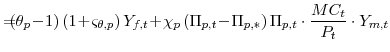
The first-order condition from the intermediate goods producing firms profit-maximization problem (equation 9), the aggregate supply curver, is:

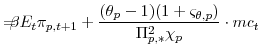
$\displaystyle \theta_{p}\cdot\frac{MC_{t}}{P_{t}}\cdot Y_{f,t} \!\!\!\!$	$\displaystyle =\!\!\!\! (\theta_{p}\!-\!1)\left( 1\!+\!\varsigma_{\theta,p} \right) Y_{f,t} \!+\!\chi_{p}\left( \Pi_{p,t}\!-\!\Pi_{p,\ast}\right) \Pi_{p,t}\cdot \frac{MC_{t}}{P_{t}}\cdot Y_{m,t}$
$\displaystyle$	$\displaystyle -\!\!\!\!\beta E_{t} \left[ \frac{\Lambda_{c,t+1}}{\Lambda_{c,t}% }\cdot\chi_{p}\left( \Pi_{p,t+1}\!-\!\Pi_{p,\ast}\right) \Pi_{p,t+1}% \cdot\frac{MC_{t+1}}{P_{t+1}}\cdot Y_{m,t+1}\right]%$	(17)

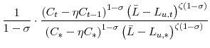
The first-order conditions from the household's utility-maximization problem (equation 10), the Euler equation and the labor supply curve, are:

$\displaystyle \frac{\Lambda_{c,t}}{P_{t}} \!\!\!\!$	$\displaystyle =\!\!\!\!\beta R_{t} E_{t}\left[ \frac{\Lambda_{c,t+1}}{P_{t+1}} \right]$	(18)
$\displaystyle \theta_{w}\cdot\frac{\Lambda_{l,t}}{\Lambda_{c,t}}\cdot L_{y,t} \!\!\!\!$	$\displaystyle =\!\!\!\! \left( \theta_{w}\!-\!1\right) \left( 1\!+\!\varsigma_{\theta,w} \right) \frac{W_{t}}{P_{t}}\cdot L_{y,t} \!+ \!\chi_{w} \left( \Pi _{w,t}\!-\!\Pi_{w,\ast}\right) \Pi_{w,t}\cdot\frac{\Lambda_{l,t}}% {\Lambda_{c,t}}\cdot L_{u,t}$
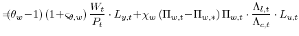
$\displaystyle$	$\displaystyle -\!\!\!\!\beta E_{t} \left[ \frac{\Lambda_{c,t+1}}{\Lambda_{c,t}% }\cdot\chi_{w} \left( \Pi_{w,t+1}\!-\!\Pi_{w,\ast}\right) \Pi_{w,t+1}% \cdot\frac{\Lambda_{l,t+1}}{\Lambda_{c,t+1}}\cdot L_{u,t+1}\right]%$	(19)

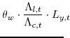
where

$\displaystyle \Lambda_{c,t} \!\!\!\!$	$\displaystyle =\!\!\!\!\left( C_{t}\!-\!\eta C_{t-1}\right) ^{\!-\sigma} \!\left( \bar{L}\!-\!L_{t}\right) ^{\!\zeta(1\!-\!\sigma)} \!-\!E_{t}\beta\eta\!\left[ \left( C_{t+1}\!-\!\eta C_{t}\right) ^{\!-\sigma} \!\left( \bar{L}\!-\!L_{t+1}\right) ^{\!\zeta(1\!-\!\sigma)}\right]$	(20)
$\displaystyle \Lambda_{l,t} \!\!\!\!$	$\displaystyle =\!\!\!\!\zeta\left( C_{t}\!-\!\eta C_{t-1}\right) ^{(1\!-\!\sigma)} \left( \bar{L}\!-\!L_{t}\right) ^{\zeta(1\!-\!\sigma )-1}.%$	(21)

The model has three market clearing conditions: the labor market clearing condition, the intermediate-goods market clearing condition, and the final-goods market clearing condition. In the symmetric equilibrium these are given by:

$\displaystyle L_{u,t}\!\!\!\!$	$\displaystyle =\!\!\!\!L_{y,t} +\frac{\chi_{w}}{2} \left( \Pi_{w,t}% -\Pi_{w,t-1} \right) ^{2}L_{u,t},$	(22)
$\displaystyle Y_{f,t}\!\!\!\!$	$\displaystyle =\!\!\!\!Y_{m,t} -\frac{\chi_{p}}{2} \left( \Pi_{p,t}% -\Pi_{p,t-1} \right) ^{2}Y_{m,t},$	(23)
$\displaystyle C_{t}\!\!\!\!$	$\displaystyle =\!\!\!\!Y_{f,t}%$	(24)

A..2 Log-linearized first-order conditions

The first-order conditions implied by the intermediate goods producing firm's cost minimization problem, given by equations (15) and (16), log-linearize to

$\displaystyle l_{y,t}\!\!\!\!$	$\displaystyle =\!\!\!\!y_{m,t}-a_{t}$	(25)
$\displaystyle mc_{t}\!\!\!\!$	$\displaystyle =\!\!\!\!w_{t}-a_{t}%$	(26)

The first-order conditions implied by the intermediate goods producing firm's profit maximization problem, given by equation (17), log-linearizes to

$\displaystyle \pi_{p,t}\!\!\!\!$	$\displaystyle =\!\!\!\!\beta E_{t}\pi_{p,t+1} +\frac{(\theta _{p}-1)(1+\varsigma_{\theta,p})}{\Pi^{2}_{p,\ast}\chi_{p}} \cdot mc_{t}$
$\displaystyle$	$\displaystyle =\!\!\!\!\beta E_{t}\pi_{p,t+1} +\kappa_{p} \cdot mc_{t}% %$	(27)

The first-order conditions implied by the household's utility maximization problem, given by equations (18) and (19), log-linearize to:

$\displaystyle \lambda_{c,t}\!\!\!\!$	$\displaystyle =\!\!\!\!r_{t}-E_{t}\pi_{p,t+1}+E_{t}\lambda _{c,t+1}$	(28)
$\displaystyle \pi_{w,t}\!\!\!\!$	$\displaystyle =\!\!\!\!\beta E_{t}\pi_{w,t+1} +\frac{(\theta _{w}-1)(1+\varsigma_{\theta,w})}{\Pi^{2}_{w,\ast}\chi_{w}} \cdot\left( \lambda_{l,t}-\lambda_{c,t}-w_{t}\right)$
$\displaystyle$	$\displaystyle =\!\!\!\!\beta E_{t}\pi_{w,t+1} +\kappa_{w} \cdot\left( \lambda_{l,t}-\lambda_{c,t}-w_{t}\right)%$	(29)

where

$\displaystyle \lambda_{c,t}\!\!\!\!$	$\displaystyle =\!\!\!\! \frac{1}{1\!-\!\eta\beta} \left( \frac{-\sigma}{1\!-\!\eta}\left( c_{t}\!-\!\eta c_{t-1}\right) \!-\!\zeta (1\!-\!\sigma)\frac{L_{u,\ast}}{\bar{L}\!-\!L_{u,\ast}}\cdot l_{u,t}\right)$
	$\displaystyle - \frac{\eta\beta}{1\!-\!\eta\beta} \! \left( \!\frac{-\sigma}{1\!-\!\eta} \!\left( E_{t} c_{t+1}\!-\!\eta c_{t}\right) \!-\!\zeta(1\!-\!\sigma)\frac{L_{u,\ast}}{\bar{L}\!-\!L_{u,\ast}} \cdot E_{t} l_{u,t+1} \!\right)$	(30)
$\displaystyle \lambda_{l,t}\!\!\!\!$	$\displaystyle =\!\!\!\! \frac{1-\sigma}{1-\eta} \left( c_{t}-\eta c_{t-1} \right) +\left( 1-\zeta\left( 1-\sigma\right) \right) \frac {L_{u,\ast}}{\bar{L}-L_{u,\ast}}\cdot l_{u,t}.%$	(31)

The market clearing conditions, equations (22), (23), and (24), log-linearize to:

$\displaystyle l_{u,t}\!\!\!\!$	$\displaystyle =\!\!\!\!l_{y,t}=l_{t}$	(32)
$\displaystyle y_{f,t}\!\!\!\!$	$\displaystyle =\!\!\!\!y_{m,t}=y_{t}$	(33)
$\displaystyle c_{t}\!\!\!\!$	$\displaystyle =\!\!\!\!y_{f,t}%$	(34)

Three more equations remain in our model: (i) the process for the shocks $A_{t}$ , defined in equation (4), which log-linearizes to:

$\displaystyle a_{t}=a_{t-1}+\epsilon_{t},%$

(35)

(ii) the monetary policy process, which was already given in log-linearized form in section 3.2, and (iii) an identity between price and wage inflation and real wages:

$\displaystyle \frac{W_{t}}{P_{t}}\cdot\frac{P_{t-1}}{W_{t-1}} =\frac{W_{t}}{W_{t-1}}% \cdot\frac{P_{t-1}}{P_{t}}=\frac{\Pi_{w,t}}{\Pi_{p,t}}$

which log-linearized to:

$\displaystyle w_{t}-w_{t-1}=\pi_{w,t}-\pi_{p,t}$

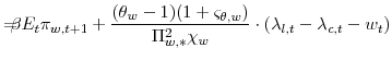
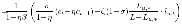
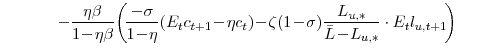
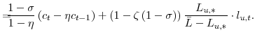
Before concluding this section we note the following about the steady-state solution to the model. We know from equations (16), (17), (19), (20), and (21) that in the steady state:

$\displaystyle 1=\frac{MC_{\ast}}{P_{\ast}}=\frac{W_{\ast}}{P_{\ast}}=\frac{\Lambda_{l,\ast}% }{\Lambda_{c,\ast}} =\frac{1-\eta}{1-\eta\beta}\cdot\frac{\zeta L_{u,\ast}% }{\bar{L}-L_{u,\ast}}$

Since $L_{\ast}=L_{u,\ast}=L_{y,\ast}$ we can re-write this as:

$\displaystyle \frac{\zeta L_{\ast}}{\bar{L}-L_{\ast}}=\frac{1-\eta\beta}{1-\eta }.%$

(36)

This means that we can re-write equations (30) and (31) as:

$\displaystyle \lambda_{c,t}\!\!\!\!$	$\displaystyle =\!\!\!\! \frac{1}{1\!-\!\eta\beta} \left( \frac{-\sigma}{1\!-\!\eta}\left( c_{t}\!-\!\eta c_{t-1}\right) \!-\!(1\!-\!\sigma)\frac{1-\eta\beta}{1-\eta}\cdot l_{u,t}\right)$
	$\displaystyle + \frac{\eta\beta}{1\!-\!\eta\beta} \! \left( \!\frac{-\sigma}{1\!-\!\eta} \!\left( E_{t} c_{t+1}\!-\!\eta c_{t}\right) \!-\!(1\!-\!\sigma)\frac{1-\eta\beta}{1-\eta} \cdot E_{t} l_{u,t+1} \!\right)$
$\displaystyle \lambda_{l,t}\!\!\!\!$	$\displaystyle =\!\!\!\! \frac{1-\sigma}{1-\eta} \left( c_{t}-\eta c_{t-1} \right) +\frac{1-\zeta\left( 1-\sigma\right) }{\zeta}\cdot \frac{1-\eta\beta}{1-\eta}\cdot l_{u,t}.$

Since $l_{u,t}=l_{y,t}=y_{m,t}-a_{t}=y_{t}-a_{t}$ and $c_{t}=y_{f,t}=y_{t}$

$\displaystyle \lambda_{c,t}\!\!\!\!$	$\displaystyle =\!\!\!\! \frac{1}{1\!-\!\eta\beta} \left( \frac{-\sigma}{1\!-\!\eta}\left( y_{t}\!-\!\eta y_{t-1}\right) \!-\!(1\!-\!\sigma)\frac{1-\eta\beta}{1-\eta}(y_{t}-a_{t})\right)$
	$\displaystyle + \frac{\eta\beta}{1\!-\!\eta\beta} \! \left( \!\frac{-\sigma }{1\!-\!\eta} \!\left( E_{t} y_{t+1}\!-\!\eta y_{t}\right) \!-\!(1\!-\!\sigma )\frac{1-\eta\beta}{1-\eta} (E_{t}y_{t+1}-E_{t}a_{t+1}) \!\right)$	(37)
$\displaystyle \lambda_{l,t}\!\!\!\!$	$\displaystyle =\!\!\!\! \frac{1-\sigma}{1-\eta} \left( y_{t}-\eta y_{t-1} \right) +\frac{1-\zeta\left( 1-\sigma\right) }{\zeta}\cdot \frac{1-\eta\beta}{1-\eta}(y_{t}-a_{t}).%$	(38)

Equations (37) and (38) will be used in deriving the natural rate.

A..3 Natural rates in the log-linear model

The natural rate of output, i.e. the level of output in the equilibrium with perfectly flexible prices and wages, is determined by the condition that the marginal rate of substitution between consumption and leisure be (up to constants) equal to the marginal product of labor at all dates . In log terms, $y^{n}_{t}$ is determined implicitly by the equation

$\displaystyle mrs_{t}=mpl_{t}%$

(39)

where $mrs_{t}=\lambda_{l,t}-\lambda_{c,t}$ and, from the production function (3), $mpl_{t}=a_{t}$ . Substituting from (37) and (38) for $\lambda_{c,t}$ and $\lambda_{l,t}$ yields the following expression for $y^{n}_{t}$ :

$\displaystyle [\delta_{1}-\delta_{2}(L+\beta L^{-1})]y^{n}_{t} = [\delta_{3}-\delta _{4}L^{-1}]a_{t}%$

(40)

where

denotes the lag operator, $L^{-1}x_{t}\equiv E_{t}x_{t+1}$ , and

$\displaystyle \delta_{1}$	$\displaystyle = \frac{2(1-\sigma)}{1-\eta} + \frac{1-\zeta(1-\sigma)}{\zeta} \frac{1-\beta\eta}{1-\eta} + \frac{\sigma(1+\beta\eta^{2})}{(1-\beta \eta)(1-\eta)}$
$\displaystyle \delta_{2}$	$\displaystyle = \eta\left[ \frac{1-\sigma}{1-\eta} + \frac{\sigma}% {(1-\beta\eta)(1-\eta)}\right]$
$\displaystyle \delta_{3}$	$\displaystyle = 1 + \frac{1-\zeta(1-\sigma)}{\zeta} \frac{1-\beta\eta}{1-\eta} + \frac{1-\sigma}{1-\eta},$ and $\displaystyle$
$\displaystyle \delta_{4}$	$\displaystyle = \frac{\beta\eta(1-\sigma)}{1-\eta}%$

The natural rate of interest, denoted $r^{n}_{t}$ , is the real rate $r_{t}-E_{t}\pi_{t+1}$ prevailing in the equilibrium with perfectly flexible prices and wages. Letting $\lambda^{n}_{c,t}$ denote the expression (37) with $y^{n}_{t}$ substituted for $y_{t}$ , the Euler equation (28) in this equilibrium can be expressed as

$\displaystyle r^{n}_{t}=\lambda^{n}_{c,t}-E_{t}\lambda^{n}_{c,t+1}%$

(41)

But, in this equilibrium, $\lambda^{n}_{c,t}=\lambda^{n}_{l,t}-a_{t}$ . Substituting for $\lambda^{n}_{c,t}$ we obtain

$\displaystyle r^{n}_{t}$	$\displaystyle = [\delta_{6}+\delta_{7}-\delta_{6} L-\delta_{7} L^{-1}] y^{n}_{t} + \delta_{8}[L^{-1}-1]a_{t}$
	$\displaystyle = \delta_{6} \Delta y^{n}_{t} - \delta_{7} E_{t} \Delta y^{n}_{t+1} + \delta_{8}E_{t} \Delta a_{t+1}%$	(42)

with

$\displaystyle \delta_{6}$	$\displaystyle = \frac{\eta(1-\sigma)}{1-\eta}$
$\displaystyle \delta_{7}$	$\displaystyle = \frac{1-\sigma}{1-\eta} + \frac{1-\zeta(1-\sigma)}{\zeta} \frac{1-\beta\eta}{1-\eta}$
$\displaystyle \delta_{8}$	$\displaystyle = 1+ \frac{1-\zeta(1-\sigma)}{\zeta} \frac{1-\beta\eta}{1-\eta}%$

B. VAR Identification and Structural Shocks

As discussed in section 3, we are interested in matching the VAR's impulse responses to two of the structural shocks of our model, a permanent shock to the level of technology, and a transitory shock to the funds rate. To identify these shocks, we use one long-run and one short-run identifying restriction. The short-run identifying restriction is the usual one, that the last variable in the VAR (the funds rate) is Wold-causal for the preceding variables. The structural form of the VAR is given by

$\displaystyle A_{0}Y_{t}={\mathit{constant}}+A(L)Y_{t-1}+\varepsilon_{t},$

(43)

where $Y_{t}$ is defined in (13). The short-run assumption implies that the last column of the contemporaneous multiplier matrix $A_{0}$ has all zeros above the main diagonal. The fifth element of $\varepsilon_{t}$ is identified as the funds rate shock $\epsilon_{r,t}$ in the policy rule. The long-run identifying restriction is the one proposed by Galí (1999) and further explored in Francis and Ramey (2005) and Altig et al. (2002), that permanent shocks to technology are the only shocks to have a permanent effect on labor productivity. Using this assumption, we identify the first element of $\varepsilon_{t}$ as the technology shock $\epsilon_{t}$ in (4). This implies that the first row of the matrix of long-run (cumulative) effects of $\varepsilon_{t}$ on $Y_{t}$ , $(I-A(1))^{-1}A_{0}% ^{-1}$ , consists of zeros except for the first element.

In order to estimate the VAR in structural form, we need a further set of assumptions to just-identify the elements of $A_{0}$ . We follow Altig et al. (2002) by assuming that the submatrix consisting of columns 2-4 and rows 2-4 of $A_{0}$ is lower triangular. This assumption is without loss of generality as we do not attach any structural interpretation to elements 2 through 4 of $\varepsilon_{t}$ . With these assumptions, we estimate the first equation of the structural VAR imposing the long-run restrictions in the manner of Shapiro and Watson (1988) by including contemporaneous and lagged variables of elements 2 through 4 of $Y_{t}$ in first-differenced form. To control for simultaneity, we estimate the equation by 2SLS, using a constant and $Y_{t-1},\ldots,Y_{t-4}$ as first-stage regressors for elements 2 through 4 of $Y_{t}$ . We then sequentially estimate equations 2 through 4 by IV, using the residuals from the previous regressions as instruments for contemporaneous variables. Equation 5 can be estimated by OLS by virtue of our short-run identifying assumption.

We modify this identification strategy in one respect. Because, in contrast to Altig et al., our VAR includes hours per capita in first differences, we would like to assure that the long-run response of hours to a technology shock is zero, consistent with the observation that hours worked have remained broadly unchanged despite the secular trend in real wages. When this second long-run restriction is not imposed, the IRF of $\Delta l$ usually does not integrate to zero. We therefore reorder our vector of endogenous variables to include $\Delta l$ as the second variable, and apply the Shapiro-Watson method to the first two equations. This leaves the interpretation of the first element of $\varepsilon_{t}$ unchanged, but the second element is now the only shock that permanently affects hours per capita. Contrary to the findings reported by Francis and Ramey (2005), Laubach and Williams (2006) find that imposing this second long-run restriction can have a substantial effect on the response of hours to a technology shock.

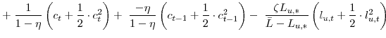
C. Deriving the Welfare Criterion

To derive the welfare criterion we first take a second-order approximation to the within-period utility function

	$\displaystyle \frac{1}{1-\sigma}\cdot\frac{\left( C_{t}-\eta C_{t-1}\right) ^{1-\sigma}\left( \bar{L}-L_{u,t}\right) ^{\zeta(1-\sigma)}} {\left( C_{\ast}-\eta C_{\ast}\right) ^{1-\sigma}\left( \bar{L}-L_{u,\ast}\right) ^{\zeta(1-\sigma)}}$
$\displaystyle$	$\displaystyle = \mathrm{T.I.P.}$
$\displaystyle$	$\displaystyle +\; \frac{1}{1-\eta} \left( c_{t}+\frac{1}{2}\cdot c^{2}% _{t}\right) +\; \frac{-\eta}{1-\eta} \left( c_{t-1}+\frac{1}{2}\cdot c^{2}_{t-1}\right) -\; \frac{\zeta L_{u,\ast}}{\bar{L}-L_{u,\ast}} \left( l_{u,t}+\frac{1}{2}\cdot l^{2}_{u,t}\right)$
$\displaystyle$	$\displaystyle +\; \frac{1}{2}(-\sigma) \frac{1}{1-\eta}\cdot\frac{1}{1-\eta} \left( c_{t}+\frac{1}{2}\cdot c^{2}_{t}\right) \left( c_{t}+\frac{1}{2}\cdot c^{2}_{t}\right)$
$\displaystyle$	$\displaystyle +\; \frac{1}{2}(-\sigma) \frac{-\eta}{1-\eta}\cdot\frac{-\eta }{1-\eta} \left( c_{t-1}+\frac{1}{2}\cdot c^{2}_{t-1}\right) \left( c_{t-1}+\frac{1}{2}\cdot c^{2}_{t-1}\right)$
$\displaystyle$	$\displaystyle -\; \frac{1}{2}\cdot\frac{1-\zeta(1-\sigma)}{\zeta}\cdot\frac{\zeta L_{u,\ast}}{\bar{L}-L_{u,\ast}}\cdot\frac{\zeta L_{u,\ast}}{\bar{L}-L_{u,\ast }} \left( l_{u,t}+\frac{1}{2}\cdot l^{2}_{u,t}\right) \left( l_{u,t}+\frac {1}{2}\cdot l^{2}_{u,t}\right)$
$\displaystyle$	$\displaystyle +\; (-\sigma) \frac{1}{1-\eta}\cdot\frac{-\eta}{1-\eta} \left( c_{t}+\frac{1}{2}\cdot c^{2}_{t}\right) \left( c_{t-1}+\frac{1}{2}\cdot c^{2}_{t-1}\right)$
$\displaystyle$	$\displaystyle -\; (1-\sigma) \frac{1}{1-\eta}\cdot\frac{\zeta L_{u,\ast}}{\bar {L}-L_{u,\ast}} \left( c_{t}+\frac{1}{2}\cdot c^{2}_{t}\right) \left( l_{u,t}+\frac{1}{2}\cdot l^{2}_{u,t}\right)$
$\displaystyle$	$\displaystyle -\; (1-\sigma) \frac{-\eta}{1-\eta}\cdot\frac{\zeta L_{u,\ast}% }{\bar{L}-L_{u,\ast}} \left( c_{t-1}+\frac{1}{2}\cdot c^{2}_{t-1}\right) \left( l_{u,t}+\frac{1}{2}\cdot l^{2}_{u,t}\right)%$	(44)

We also make use of the quadratic approximations to the labor demand curve (equation 15) and the market clearing conditions (equations 23, 22, and 24) which are given by:

$\displaystyle \left( l_{y,t}+\frac{1}{2}\cdot l^{2}_{y,t}\right) \!\!\!\!$	$\displaystyle =\!\!\!\!\left( y_{m,t}+\frac{1}{2}\cdot y^{2}_{m,t}\right) -\left( a_{t}+\frac{1}{2}\cdot a^{2}_{t}\right) -y_{m,t}a_{t}$
$\displaystyle \left( l_{y,t}+\frac{1}{2}\cdot l^{2}_{y,t}\right) \!\!\!\!$	$\displaystyle =\!\!\!\!\left( l_{u,t}+\frac{1}{2}\cdot l^{2}_{u,t}\right) -\frac{1}{2}\cdot\chi_{w} \cdot\Pi_{w,\ast}^{2} \pi_{w,t}^{2}$
$\displaystyle \left( y_{f,t}+\frac{1}{2}\cdot y^{2}_{f,t}\right) \!\!\!\!$	$\displaystyle =\!\!\!\!\left( y_{m,t}+\frac{1}{2}\cdot y^{2}_{m,t}\right) -\frac{1}{2}\cdot\chi_{p} \cdot\Pi_{p,\ast}^{2} \pi_{p,t}^{2}$
$\displaystyle \left( c_{t}+\frac{1}{2}\cdot c^{2}_{t}\right) \!\!\!\!$	$\displaystyle =\!\!\!\!\left( y_{f,t}+\frac{1}{2}\cdot y^{2}_{f,t}\right)$

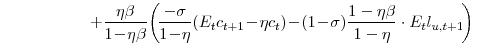
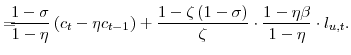
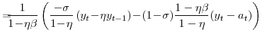
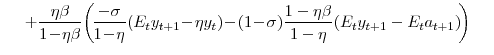
Substituting the above equations into the equation (44) and making a number of substitutions yields:

	$\displaystyle \frac{1}{1-\sigma}\cdot\frac{\left( C_{t}-\eta C_{t-1}\right) ^{1-\sigma}\left( \bar{L}-L_{u,t}\right) ^{\zeta(1-\sigma)}} {\left( C_{\ast}-\eta C_{\ast}\right) ^{1-\sigma}\left( \bar{L}-L_{u,\ast}\right) ^{\zeta(1-\sigma)}}$
	$\displaystyle = \mathrm{T.I.P.}$
	$\displaystyle -\; \frac{1}{2} \cdot\sigma\left( \frac{1}{1-\eta}\right) ^{2} \left( \left( y_{t}-y^{n}_{t}\right) -\eta\left( y_{t-1}-y^{n}_{t-1}\right) \right) ^{2}$
	$\displaystyle -\; \frac{1}{2} \cdot\frac{1-\zeta(1-\sigma)}{\zeta} \cdot\left( \frac{1-\beta\eta}{1-\eta} \right) ^{2} \left( y_{t}-y^{n}_{t}\right) ^{2}$
	$\displaystyle -\; (1-\sigma)\cdot\frac{1-\beta\eta}{1-\eta}\cdot\frac{1}{1-\eta}% \cdot\left( y_{t}-y^{n}_{t}\right) \left( \left( y_{t}-y^{n}_{t}\right) -\eta\left( y_{t-1}-y^{n}_{t-1}\right) \right)$
	$\displaystyle -\; \frac{1}{2}\cdot\frac{1-\beta\eta}{1-\eta} \left\{ \chi_{p}\Pi_{p,\ast }^{2}\pi_{p,t}^{2} +\; \chi_{w}\Pi_{w,\ast}^{2}\pi_{w,t}^{2}\right\} .$

Letting $x_{t}\equiv y_{t}-y^{n}_{t}$ , and taking account our expressions for $\kappa_{p}$ and $\kappa_{w}$ this can also be written as:

	$\displaystyle \frac{1}{1-\sigma}\cdot\frac{\left( C_{t}-\eta C_{t-1}\right) ^{1-\sigma}\left( \bar{L}-L_{u,t}\right) ^{\zeta(1-\sigma)}} {\left( C_{\ast}-\eta C_{\ast}\right) ^{1-\sigma}\left( \bar{L}-L_{u,\ast}\right) ^{\zeta(1-\sigma)}}$
	$\displaystyle = \mathrm{T.I.P.}$
	$\displaystyle -\; \frac{1}{2} \cdot\sigma\left( \frac{1}{1-\eta}\right) ^{2} \left( x_{t}-\eta\;x_{t-1}\right) ^{2}$
	$\displaystyle -\; \frac{1}{2} \cdot\frac{1-\zeta(1-\sigma)}{\zeta} \cdot\left( \frac{1-\beta\eta}{1-\eta} \right) ^{2} x_{t}^{2}$
	$\displaystyle -\; (1-\sigma)\cdot\frac{1-\beta\eta}{1-\eta}\cdot\frac{1}{1-\eta}\cdot x_{t} \left( x_{t}-\eta\;x_{t-1}\right)$
	$\displaystyle -\; \frac{1}{2}\cdot\frac{1-\beta\eta}{1-\eta} \left\{ \frac{\theta_{p}% }{\kappa_{p}}\pi_{p,t}^{2} +\; \frac{\theta_{w}}{\kappa_{w}}\pi_{w,t}% ^{2}\right\} ,$

which is the equation given in section 4 of the paper.

Footnotes

* Board of Governors of the Federal Reserve System, [email protected]; Board of Governors of the Federal Reserve System, [email protected]; and Federal Reserve Bank of San Francisco, [email protected] (corresponding author). We thank Richard Dennis, Petra Geraats, Andy Levin, Chris Sims, Ulf Söderström, and participants at the Federal Reserve Bank of San Francisco Conference on "Monetary Policy, Transparency, and Credibility" and seminars at the European Central Bank, Humboldt Universität Berlin, and the Federal Reserve Board for comments. The views expressed herein are those of the authors and do not necessarily reflect those of the Board of Governors of the Federal Reserve System, its staff, or the management of the Federal Reserve Bank of San Francisco. Return to Text

1. Basu and Kimball (2002) argue that nonseparability between consumption and leisure has substantial empirical support. Return to Text

2. We acknowledge that such a subsidy is not in effect in practice, implying that in the real world the steady-state level of output is inefficient. We leave to future work the study of optimal policy under parameter uncertainty in an economy characterized by a distorted steady-state allocation. Return to Text

3. For various reasons, our approach may over- or under-estimate the degree of parameter uncertainty that a policymaker faces. The extent to which the posterior distribution is generically "narrower" or "wider" than we estimate will primarily affect the quantitative aspect of out results, not the qualitative nature. Return to Text

4. Applications of this estimation strategy are found in Rotemberg and Woodford (1997), Amato and Laubach (2003), and Christiano, et al (2005). This estimation methodology remains the subject of considerable controversy. In particular, it has been criticized for the use of a ad hoc selection criteria for the moments that are used in the estimation. In addition, Canova and Sala (2006) highlight the problem of weak identification of some model parameters using this method, a problem that is also present with other estimation strategies. Return to Text

5. By contrast, Altig et al. (2002) and Galí, López-Salido, and Vallés (2003) compute labor productivity by dividing real GDP by total hours in the nonfarm business sector, which could be problematic because of the trending share of nonfarm business output in GDP. Return to Text

6. Note that we include log hours per capita in first differences in the VAR in order to avoid contamination of our estimation results from the apparent nonstationarity in log hours per capita. See Francis and Ramey (2005) and Altig et al. (2002) for further discussion of this contentious issue. Return to Text

7. To prevent the standard error bands from diverging over time, we discard draws for which the implied reduced-form VAR was estimated to be unstable, such as draws for which the largest eigenvalue of the coefficient matrix in the reduced form, written in companion form, exceeds .99. In total, about 14 percent of all draws are being rejected. Return to Text

8. Preliminary estimation results indicated a slightly negative, but near zero, response of monetary policy to the output gap, perhaps because the theoretical notion of the output gap in our model bears little resemblance to measures of the output gap used by policymakers. In the results reported in the paper, we constrained the response to the output gap to zero. Return to Text

9. For sticky prices the relationship between the coefficient on the driving process in the price Phillips curve, $\kappa_{p}$ , and the coefficient on price inflation variability in the loss function is identical for the alternative assumption of Calvo pricing. For sticky wages, however, the relationship is not invariant; in particular, under Calvo-style wage setting, an additional term, equal to $\left( 1+\theta_{w}\left( \frac{1-\zeta\left( 1-\sigma\right) }{\zeta}\right) \left( \frac{1-\beta \eta}{1-\eta}\right) \right)$ multiplies the coefficient on wage inflation variability in the loss function. Return to Text

10. Clearly, the relative weights shown in Table 2 are sensitive to our nominal rigidity assumptions. As discussed in the preceding footnote, the assumption of Calvo contracts would scale up significantly the relative weight on wage inflation, while, as documented by Dixon and Kara (2006), the assumption of Taylor contracts would make the relative weight on the output gap about three times larger (relative to the weights on price and wage inflation) than under Calvo contacts. Return to Text

11. Based on the point estimates, the weights on the squared level of the output gap and the squared quasi-difference of the output gap are about equal, while that on the cross-product is smaller and has the opposite sign. Return to Text

12. The welfare losses are in absolute terms. If measured in permanent consumption equivalent units, these losses are very small, reflecting the fact that we are only considering one source of shocks to the economy. Return to Text

13. In the presence of other shocks, the optimal policy likely produces interest rate variability so great that the zero lower bound on nominal interest rate surely becomes a relevant concern. We leave the analysis incorporating this constraint to future work. Return to Text

14. In the two cases where this upper bound is a binding constraint, the loss surface is nearly flat in the vicinity of the reported parameter values. In the case of the Taylor Rule, increasing the upper bound to 10,000 has no effect on the loss (at three decimal places); in the case of the rule that only responds to wage and price inflation, relaxing the constraint lowers the loss from 1.760 to 1.758, the same as that under the fully optimal policy (at three decimal places). Return to Text

15. The assumption that the policymaker is certain about the correctness of the estimation methodology likely reduces the degree of parameter uncertainty relative to what policymakers face in reality. For example, in the model used in this paper, some parameter point estimates can vary significantly, depending on sample and specifics of the estimation method. We leave the study of this broader form of estimation uncertainty to future work. Return to Text

16. Indeed, Laubach and Williams (2003) find evidence of considerable uncertainty regarding low-frequency components of natural rates of interest and output, suggesting that the assumption that the steady-state levels are known with certainty is untenable in practice. Return to Text

17. In principle, the central bank could use other methods to estimate the natural rates that take into account parameter uncertainty, but basing the central bank estimates on those implied by the parameter point estimates seems a reasonable benchmark for our analysis. Return to Text

18. For this experiment, we computed the optimal coefficients of the Taylor rule under parameter uncertainty, but assumed that the central bank's estimate of natural rates are always exactly correct. The optimized coefficient on inflation is zero and that on the output gap is 1,000 (the imposed upper bound). The resulting mean welfare loss under these assumptions is 4.060. Return to Text

^♣ This version is optimized for use by screen readers. Descriptions for all mathematical expressions are provided in LaTex format. A printable pdf version is available. Return to Text

Welfare-Maximizing Monetary Policyunder Parameter Uncertainty

Welfare-Maximizing Monetary Policy
under Parameter Uncertainty