Skip to: [Printable Version (PDF)] [Bibliography] [Footnotes]

Finance and Economics Discussion Series: 2011-25 Screen Reader version ^♣

Household Income Uncertainties Over Three Decades

James Feigenbaum* and Geng Li**

March 2011

Keywords: Income uncertainty, Great Moderation, precautionary saving

Abstract:

We study the trend in household income uncertainty using a novel approach that measures income uncertainty as the variance of forecast errors at each future horizon separately without imposing parametric restrictions on the underlying income shocks. We find that household income uncertainty has risen significantly and persistently since the early 1970s. For example, our measure of near-future uncertainty in total family non-capital income rose about 40 percent between 1971 and 2002. This rising uncertainty is likely due to the increase in variances of both persistent and transitory income shocks. Although the increase in uncertainty was widespread, the increase was most pronounced among single-earner households and high-income households. A parsimoniously calibrated Aiyagari (1994) model is solved to illustrate how rising income uncertainty affects aggregate saving.

JEL Classification: D31, E21

1 Introduction

Recent studies of aggregate data find that the volatility of U.S. GDP growth declined substantially from the mid-1980s to the mid-2000s, a phenomenon dubbed as the "Great Moderation" in the literature (Kim and Nelson 1999 and McConnell and Perez-Quiros 2000). By contrast, the observation that household income volatility rose over the same period of time has been documented in a distinct line of work (see, for example, Dynan, Elmendorf, and Sichel 2007, Keys 2008, and Jensen and Shore 2010). However, few studies have focused how household income uncertainty evolved during this period. This is somewhat surprising because on the one hand, it is well known that many decisions made by households, such as consumption, savings, investment portfolio choices, and durable goods purchases, crucially depend on the uncertainty they face regarding their future income. On the other hand, though related, the evolution of income volatility does not necessarily speak to the dynamics of household income uncertainties.

Why is income volatility not equivalent to income uncertainty? To be clear, other terms-"instability," "transitory variance," and "year-to-year earnings variability" -have also been used in the literature loosely referring to income volatility. Formally, the distinction between uncertainty and these other terms is the information set upon which they are derived. Intuitively, volatility is largely a variable of macroeconomic interest, characterizing movements in the observed distribution of income, whereas uncertainty is what matters to the individual. As Cunha, Heckman, and Navarro (2005), Blundell, Pistaferri, and Preston (2008), and Shin and Solon (2010) have argued, it is important to distinguish predictable income changes from those unpredictable to households in order to accurately characterize the income risks they face.

Models that try to filter out predictable income changes are often estimated conditional on information concurrent to the realization of the income (as in Carroll and Samwick 1998 and Gottschalk and Moffitt 2008). Income uncertainty, in contrast, should refer to the risks associated with future income perceived by households conditional on the information they have at the time when they make the relevant decision.

This paper addresses these limitations and studies the trend in income uncertainty since the early 1970s using a novel approach introduced by Feigenbaum and Li (2011) that measures income uncertainty as the variance of forecast errors that households appear to face at various future horizons. This approach makes several key innovations relative to the existing workhorse models that deal with income riskiness. First, although forecast errors are constructed using a linear projection equation, we do not impose any further restrictions on the statistical properties of the forecast errors, such as how they are correlated across forecast horizons, thereby retaining the highest degree of flexibility in characterizing income uncertainty and how it changes over time. In particular, we do not presume that forecast errors can be parsimoniously decomposed into a permanent and a transitory component. Instead, we separately construct forecast errors at different future horizons that range from one year ahead to ten years ahead and estimate the variances of the forecast errors and their correlations across forecast horizons. Second, we project time income using only the information observable at time , instead of at . We also experiment with complementing this information set with selected elements in the information set observable at , acknowledging that households may have more information about their own future than an econometrician does concurrently. Although the information set we use still does not fully replicate the true information set the households use in forming the expectations of their future income, we argue that this is an important step toward studying income risks using feasible information.

Following Carroll and Samwick (1998), we focus on the uncertainty of total family non-capital income because this broad measure of income is presumed to be the most relevant type of income for models of intertemporal optimization and precautionary saving that we revisit later in the paper. Using data from the Panel Study of Income Dynamics, we first present the trends in family non-capital income uncertainty at future horizons up to 10 years ahead from the early 1970s. For example, 2-year-ahead family non-capital income uncertainty, on net, rose about 40 percent from the early 1970s to the early 2000s. In addition, our analysis shows that since the early 1970s, income uncertainty rose more at farther horizons than at nearer horizons but the persistence of forecast errors was little changed, suggesting the increase in income uncertainty cannot be solely accounted for by the increase in variances of transitory income shocks.

We then study whether income uncertainty dynamics over the last three decades demonstrated any patterns that are different based on household economic status or demographic characteristics. We find the rise of income uncertainty is widespread and is not concentrated within any specific subpopulation. Nevertheless, certain groups of households have experienced larger percentage increases in uncertainty than others. Among those groups for which income uncertainty has risen the most (in a relative sense) are single-earner households and households in the top income quartile. Further, we show that the trends we document are robust to a number of alternative model and sample specifications.

We complete our analysis by computing how much of a change in aggregate behavior should have occurred in response to this change in idiosyncratic uncertainty. Our empirical estimates of the dynamics of income uncertainty, though highly flexible, are computationally difficult to be incorporated in a standard model. We therefore solve for the equilibrium in two Aiyagari (1994) economies where the income process is (parsimoniously) calibrated to match the beginning-of-sample and end-of-sample levels of income uncertainty of our estimates, respectively. Our calibration exercise yields clear evidence of an increase in the variances of both the persistent and transitory shocks. We find that aggregate saving is 3% higher in the economy with greater income uncertainty, where the part of the saving due to precautionary reasons is more than 30% higher. This result presents a counterfactual with respect to the aggregate saving rate observed in the data, which decreased appreciably during this period. The difference between the data and the model economy calls for future research to identify other mechanisms that may have potentially discouraged saving over time to a greater degree than precautionary motives should have encouraged saving.

2 Household Income Volatility and Uncertainty

2.1 Evidence of Rising Household Income Volatility

Kim and Nelson (1999) and McConnell and Perez-Quiros (2000) convincingly demonstrate that the volatility of U.S. output growth declined sharply after the early 1980s. Using different statistical approaches, both papers identify the break date was the first quarter of 1984.¹ Similarly, Stock and Watson (2002) document that over the four decades between 1960 and 2001, the standard deviation of U.S. GDP growth declined nearly 40 percent, from an average of 2.7 % before the 1984:1 break date to an average of 1.6% after the break date. More recently, Dynan, Elmendorf, and Sichel (2006) report that standard deviations of log differences of the aggregate earnings in the National Income and Product Account (NIPA) decreased by more than 30 percent before and after this break date.

As the findings of declines in aggregate volatility proved to be robust and became widely accepted, another consensus emerged in a fast-growing literature that the volatility of household income: instead of having declined with macroeconomic volatility, household-level income volatility has increased substantially since the 1970s. Roughly speaking, there are two statistical approaches used in the literature for studying trends in household income volatility. One approach first filters out the predictable part of income by regressing household income on demographic characteristics concurrent to the income data and assumes the residuals of this regression follow some parameterized statistical process. Typically, these models assume the residuals are the sum of permanent and transitory income shocks. The variances of these shocks can be identified by examining the auto-covariance structure of these residuals in longitudinal data. Such an approach has been widely used in the precautionary saving literature (see, for example, Carroll and Samwick 1997 and Gourinchas and Parker 2002). Using this approach, Moffitt and Gottschalk (2008) find that the transitory variance of household income increased substantially in the 1980s and stayed elevated since then.

Despite its many desirable features, the above approach has certain limitations. Notably, as Shin and Solon (2010) argue, "......the parametric models used in the literature are arbitrary mechanical constructs and the resulting estimates of trends can be sensitive to arbitrary variations in model specification." Indeed, Baker and Solon (2003) reject many restrictions that are routinely imposed on such models.

In light of such concerns, the second approach of studying income volatility takes a more agnostic stand with respect to the underlying data generation process of income shocks. For example, Dynan, Elmendorf and Sichel (2007) and Shin and Solon (2010) both use the cross-sectional dispersions in year-to-year household income growth as a measure of income volatility. The former paper finds that the volatility of various measures of household income all increased substantially since the early 1970s, albeit not at a steady pace. The latter paper, focusing on a more narrowly defined metric of income, finds that the volatility of men's labor earnings did increase in the 1970s but did not show any pronounced increase since then until the 2000s.²

2.2 Measuring Income Uncertainty

2.2.1 Conceptual Issues

Although these concepts are often interchangeably used, income volatility is not equivalent to uncertainty. Whereas income volatility is a measure of income variability in general, income uncertainty only encompasses future variability that cannot be predicted conditional on currently available information. Let $y_{t,s}$ denote the logarithm of the future income periods ahead of time . We have

$\displaystyle y_{t,s}=E\left[ y_{t,s}\vert\mathcal{I}_{t}^{H}\right] +\varepsilon _{t,s},$

(1)

where $E\left[ y_{t,s}\vert\mathcal{I}_{t}^{H}\right]$ is the component of the

-period-ahead future income that is predictable conditional on time-

information.³ Superscript

reminds us that this is the household information set, which is potentially larger than the information set an econometrician has at the same time; $\varepsilon _{t,s}$ is a shock that is orthogonal to $\mathcal{I}_{t}^{H}$ . Income uncertainty is revealed by the variance of $\varepsilon _{t,s}$ , which can vary with both

and

To be clear, income uncertainty formulated in this way is an ex post uncertainty in the sense that the level of uncertainty is estimated only after the realization of income. Later in the paper when solving for the optimal precautionary saving rate, we implicitly assume that the realized uncertainty is consistent with the ex ante perceived uncertainty. However, this assumption may not hold all the time. Two approaches, which are not the focus of this paper, can be used for a more focused study of the ex ante uncertainty. First, one may use the household choice variables to infer income uncertainty perceived by households (Guvenen and Smith 2008), although this requires more assumptions about household behavior than we are willing to make here. Second, some surveys explicitly ask participating households their estimates of the riskiness of future income, providing direct measures of ex ante income uncertainty.

From the above decomposition we have

$\displaystyle Var(y_{t,s})=Var(E\left[ y_{t,s}\vert\mathcal{I}_{t}^{H}\right] )+Var(\varepsilon _{t,s}),$

(2)

indicating that the cross-sectional variance is the sum of the variance of the predictable and unpredictable components of income-"uncertainty," as we use them. Taking the difference between $Var(y_{t,s})$ and $Var(y_{t-1,s})$ , we have

$\displaystyle \Delta Var(y_{t,s})=Var(E\left[ y_{t,s}\vert\mathcal{I}_{t}^{H}\right] )-Var(E \left[ y_{t-1,s}\vert\mathcal{I}_{t-1}^{H}\right] )+Var(\varepsilon _{t,s})-Var(\varepsilon _{t-1,s}).$

(3)

Therefore, changes in the cross-sectional variance are the same as changes in income uncertainty only if the predictability term, $Var(E\left[ y_{t,s}\vert \mathcal{I}_{t}^{H}\right] )$ , is constant over time, which is not necessarily true. For example, in the context of time series, Campbell (2007) points out that real GDP growth has become less predictable, and not taking into account the changes in predictability can lead to biased estimates of the reduction of aggregate volatilities. Similarly, the observed changes in the unconditionally measured income volatility likely do not truthfully reflect changes in uncertainty either.

Furthermore, as discussed before, the routinely used approach of filtering out predictable income is to regress the observed income on concurrent household characteristics. Essentially, this is equivalent to regressing $y_{t+s}$ on an information set that is likely observable only at time . But a household predicting its -period-ahead income at time can only use the information available to it at time . Therefore, the residuals from such a regression are more accurately interpreted as the unexplained component, rather than the unpredictable component, of income.

2.2.2 Estimation Methodology

To address the limitations of the existing methodology discussed above, this paper studies income uncertainty and its evolution over time using an approach introduced in Feigenbaum and Li (2011) that measures income uncertainty as the cross-sectional variance of forecast errors.⁴ We construct such forecast errors using a simple linear projection for each future horizon (up to 10 years ahead) and evaluate their variances in each year. For each future horizon, , we estimate the following projection equation

$\displaystyle y_{i,t,s}=\alpha ^{s}+\beta _{0}^{s}y_{i, t}+\beta _{1}^{s}y_{i,t-1}+\beta _{2}^{s}y_{i,t-2}+\gamma ^{s}Z_{i,t}+\xi ^{s}Trend_{t,s}+\varepsilon _{i,t,s},$

(4)

where household

-period-ahead income, $y_{i,t,s}$ , is projected on the information available to it at time

. Specifically, $y_{i,t}$ , $y_{i,t-1}$ , and $y_{i,t-2}$ are the household's current and lagged income. $Z_{i,t}$ is a vector of demographic characteristics and labor market status, including family size, household head's age race, marital status, education, employment status, and industry and occupation observed at time

. ⁵ We also include a linear trend $Trend_{t,s}$ that is equal to

. We then compute the variance of $\varepsilon _{i,t,s}$ for each

and

so that we can characterize how income uncertainty changed over time at various horizons without imposing parametric restrictions on underlying income shocks. In the rest of this paper, we will refer to year

as the base year and year

as the forecast year.

3 Household Income Data in the PSID

We use the Panel Study of Income Dynamics (PSID) data in our analysis. The PSID is a nationwide longitudinal survey of households conducted by the Institute of Social Research at the University of Michigan. The first wave of data was collected in 1968. It was an annual survey through 1997, and after that the PSID was restructured to a biennial survey. We use the PSID data from 1970 to 2005. We do not use the data collected in 1968 and 1969 because the exact values of head and wife transfer income, which is a component we use to compute total family non-capital income, were not collected in those two waves. The PSID has an original core nationwide representative sample of nearly 3,000 households and the sample has grown steadily since the survey was launched. An important reason for the growing sample size is that the PSID has a very high retention rate. The vast majority of households surveyed in one year continued to participate in the next wave of the survey. Indeed, there are more than 1,200 households who stayed in the survey for more than 30 years.⁶

Besides extensive information about work status, employment history and demographic characteristics, the PSID has detailed information on household income. Our study focuses on total family non-capital income. We also present statistics on the dispersion of growth of total family income and head and wife labor earnings uncertainty to facilitate comparison with the NIPA data. Both total family income and head and wife labor earnings are included in each of the PSID public releases.⁷ Family non-capital income is calculated as the sum of head and wife labor earnings, head and wife transfer income, taxable income from other family members, and transfer income from other members.⁸

To estimate Equation (4), we need to link the information of household in year , , and with the information of the same household in year for various . The number of waves each household participated in the PSID survey varies substantially. Consequently, the highly unbalanced panel limits our ability to fully explore certain longitudinal statistical properties of the sample, such as fixed or random effects. We interpret Equation (4) mainly as a statistical projection equation rather than a structural relationship. Accordingly, without loss of generality, we treat pairs of the same household in different years, such as , etc., as independent observations and pool them together to estimate the equation.⁹

We construct a sample for each projection horizon, , separately. We deflate our income measures using the CPI index with 1982-84 = 100. We then apply the following sample selection rules.

We use only the nationwide representative PSID sample and exclude the sample of low-income families and the Latino supplement sample.
We restrict the heads of our sample households to be older than 24 in the base year and younger than 65 years old in the forecast year . For example, when forecasting income five years ahead, we keep only those households whose heads are younger than 60 years old.
We keep only households whose heads reported positive labor income and positive but fewer than 4000 working hours in year , and . Furthermore, we keep only households whose heads are either working for pay, temporarily laid off or unemployed in year and , i.e. we remove the households whose heads are out of the labor force in either the base year or in the forecast year.
We keep households whose family non-capital income is positive for , , and .
Finally, we trim off the top and bottom 2.5 percent of the distribution of income growth between and in order to minimize the bias caused by outliers.¹⁰

There are two additional treatments that we apply to the PSID data. First, the PSID does not ask information about race and education in all waves, and in those years information on race and education attainments was collected, it was not carried forward for all observations, creating many blank values. We provide a remedy by replacing the blank data points of race and education with the latest valid data points prior to the blank. Doing so, we increase the sample size noticeably. Second, prior to the 2003 wave, the PSID used the 1970 census occupation and industry codes. In the 2003 and 2005 waves, the 1970 census codes were replaced with the 2000 census codes. We try our best to map the 2000 codes with the 1970 codes.

Our sample covers the PSID data from 1970 to 2005. Recalling that the year- PSID records income earned in year , our income data refer to the year of 1969 to 2004. Because Eq. (4) includes two lags of income, our estimated income uncertainty series begins in year 1971. Also, because the PSID became a biennial survey after 1997, the income uncertainty series of odd-numbered future horizons end earlier than the series of even-numbered future horizons. For example, our estimated one-year ahead uncertainty covers the period from 1971 to 1995, but the two-year ahead uncertainty series covers the period from 1971 to 2002. One additional caveat is that for the years when the PSID data were collected annually, year- income can be merged with the demographic data referring to the same year, even though they were not collected in the same wave. We do not have a perfect merge after 1997. We then use the demographic data collected in 1999, 2001, and 2003 in estimating Eq. (4) for = 1998, 2000, and 2002, respectively. For this reason, the income uncertainty in these years can be underestimated. However, because the gap is only one year and most demographic variables are highly persistent, we argue the bias is likely very small.

Table 1 reports the sizes of the samples we use to estimate Eq. (4) using family non-capital income for $1\leq s\leq 10$ . As indicated, the sample sizes generally shrink as becomes bigger because fewer households continued to participate in the PSID survey over time. Because the PSID became a biennial survey in 1997, we are no longer able to use the last several waves of data when is an odd number. Consequently, the sample for is the largest. Note also that the sample contains a comfortably large number of observations even for =10.

Table 1: Number of Observations for Each Forecast Horizon
Forecast Horizon	1 Year	2 Years	3 Years	4 Years	5 Years
Number of Observations	37,769	40,215	31,655	32,870	26,864
Forecast Horizon	6 Years	7 Years	8 Years	9 Years	10 Years
Number of Observations	26,814	22,742	21,587	19,140	17,246

Finally, we present evidence that an aggregate income approximation constructed using the PSID data does exhibit a significant decrease of volatility during the last several decades-an observation consistent with the Great Moderation-reassuring us that the PSID well represents the household sector of the aggregate economy. Following Dynan, Elmendorf and Sichel (2006), we construct the PSID sample mean income and calculate the two-year growth for the period of 1971-2004. We then compute the standard deviation of income growth over two subsamples, 1971-1985 and 1986 - 2004 and compare them with the standard deviation computed using the NIPA total personal income and employee compensations.¹¹ As table 2 shows, volatilities of both the NIPA and the PSID income measures decline appreciably between the earlier and later sample period. The most important discrepancy is that the NIPA total personal income volatility appears to have experienced an even greater decline compared with the PSID total family income.¹²

Table 2: Income Volatility in Aggregate Data
	1971 - 1985	1986 - 2004	Percent of difference
NIPA: Total personal income	3.9%	2.4%	-38.8%
NIPA: Employee compensation	5.1%	2.9%	-42.5%
PSID: Total family income	4.8%	4.1%	-14.7%
PSID: Labor earnings	4.8%	2.9%	-40.0%

4 Results

4.1 Overview of the Trend in Household Income Uncertainty

We begin by presenting an overview of the trends in family non-capital income uncertainties at both the nearer and farther horizons. Figure 1 plots the estimated 2, 4, 6, 8, and 10-year-ahead income uncertainties and their respective fitted linear trends.¹³ As we see in the top panel, the uncertainty associated with family non-capital income 2 years ahead rose substantially between 1971 and 2002. Defining the cumulative percentage-increase of income uncertainty, $\Delta \%$ , as the growth between the average within the first and the last five-year period of the sample

$\displaystyle \Delta \%=\left( \frac{\sum_{t=1971}^{1975}{Var(\varepsilon _{t,2})}}{ \sum_{t=1998}^{2002}{Var(\varepsilon _{t,2})}}-1\right) \times 100$

(5)

our estimate suggests that the 2-year-ahead income uncertainty rose nearly 40 percent during the three decades since early 1970s. Moreover, abstracting from year-to-year fluctuations, the upward trend is very persistent and prevails through the entire sample period. The two middle panels plot trends in the middle-term uncertainty of 4 and 6 years ahead. As expected, the 6-year-ahead series is higher than the 4-year-ahead uncertainty series. Similar to the 2-year-ahead uncertainty series, there is a pronounced upward trend in each of the two series. However, a pronounced decline in income uncertainty in the late 1980s is apparent in the two middle-term uncertainty series. Finally, the two bottom panels plot long-term income uncertainty. The variance of forecast errors regarding income eight years ahead rose substantially through the mid-1980s, then declined sharply before rebounding to even higher levels by the mid-1990s, the end of the series. The evolution of the 10-year-ahead income uncertainty is somewhat different. It rose through the mid-1970s, then stayed relatively flat before rising noticeably again in the later 1980s. On net, both the 8- and 10-year-ahead income uncertainty were higher at the end of the sample period than at the beginning of the sample period.

The different patterns of uncertainty dynamics across forecast horizons is partly due to varying samples used to estimate Eq. (4) when changes. In Section 5 we see that, even using a constant sample, we still find pronounced upward trends in income uncertainty across forecast horizons.

4.2 Changing Persistence or Changing Variances

Assuming the underlying income shocks can be decomposed into a purely transitory component and a more persistent (but not necessarily permanent) component, the observed rise in income uncertainties can be due to increasing transitory shock variances, increasing persistent shock variances, growing persistence of the persistent shocks, or combinations of these factors.¹⁴ We first study whether there is any evidence of growing persistence of income shocks. Figure 2 plots the correlations between the 1-year-ahead forecast errors and the 2-, 4- and 10-year-ahead forecast errors across years. If the shock persistence increased, we would expect to see these correlations also increase over time. But this is not observed in the estimated correlation series. Correlations between the 1-year-ahead forecast errors and the forecast errors of all future horizons stay flat through the mid 1990s, when our data for the 1-year-ahead forecast errors end.

Ruling out growing persistence of income shocks, we now focus on the trend in the variances of income shocks. Figure 3 plots the three-year average of the variances of the forecast errors over all future horizons ( = 1 - 10) for two periods, 1971-1973 and 1992-1994. We see that the gap between the two curves is much wider at farther horizons than at nearer horizons. This "fanning-out" pattern, holding the level of shock persistence constant, suggests that the increase in income uncertainty cannot be solely accounted for by an increase in transitory shock variances. Later in the paper, we will calibrate a parameterized income process using our estimated series of forecast error variances to assess the respective changes in the variances of transitory and persistent shocks.

4.3 Income Uncertainties for Subpopulations

We now address the question of whether the rise in income uncertainties is a widespread phenomenon or is concentrated within a subpopulation. In particular, we are interested in how trends in income uncertainty differ between dual-earner and single-earner households and across income quartiles.

First, we compare the income uncertainty of dual-earner households with that of single-earner households. The estimates of the 2-year-ahead income uncertainty profiles are presented in Figure 4. We define a household as dual-earner if the wife's labor earning is greater than 25 percent of the head's labor earning in the base year. Here, the forecast errors are constructed from estimating Eq. (4) with the whole sample but the variances of single-earner and dual-earner households are estimated separately. In Section 5 we will see that estimating Eq. (4) separately using each subpopulation does not change our results materially. As Figure 4 shows, levels of income uncertainty of single-earner and dual-earner households in the early 1970s were quite close but they diverged during the next three decades, though both series exhibit a pronounced upward trend. By the early 2000s, our cumulative uncertainty increase measure, $\Delta \%$ , is 33% for dual-earner households but 54% for single-earner households.

Figure 5 presents the 2-year-ahead income uncertainty profiles for households differentiated by quartiles of the three-year average of income over , , , where is the base year. Again, income uncertainty rose for households in all quartiles. However, the households in the highest income quartile experienced the greatest percentage increase in income uncertainty. From the lowest quartile to the highest quartile, $\Delta \%$ are 32%, 42%, 37%, and 60% respectively. Thus the percentage increase for households in the highest income quartile is much greater than other households.

Although we only presented the estimated 2-year-ahead uncertainty series for each subpopulation in Figures 4 and 5, comparison of trends in uncertainties at other future horizons over subpopulations yields the same results qualitatively. Moreover, the income uncertainty profiles of subpopulation by age (not shown) also all increased appreciably since the early 1970s.

5 Robustness Analysis

In this section, we conduct a series of analyses to ensure that the results presented above are robust to different sample selection rules as well as model specifications.

5.1 Allowing for Structural Changes in Projection Equation Parameters

One possible explanation for the rising estimated income uncertainty is that the projection relationship is not stationary over time. If the underlying true parameters of Eq. (4) change over time, the variances of forecast errors may also demonstrate time-varying patterns. To examine whether the upward trend of income uncertainty is caused by the breaks in projection relationships, we split the sample into two parts, before and after 1985. We then estimate Eq. (4) and compute the forecast error variances separately for each subsample. Although an F-test rejects the hypothesis that all coefficients are the same for each subsample, the differences are economically small. Consequently, the estimated uncertainty profiles (not shown) that allow for structural changes in parameters in the projection equations are essentially the same as those presented in Section 4.

Similarly, we estimate Eq. (4) separately for single-earner and dual-earner households and for households in each income quartile. Again, the implied income uncertainty profiles are very similar to those presented in Figures 4 and 5.

5.2 Alternative Samples

When constructing the baseline sample, we trimmed off the top and bottom 2.5% of the distribution of income growth between and . To what extent are the trends in income uncertainty affected by the tails being trimmed off? To answer this question we estimate the uncertainty profiles with two alternative samples, constructed by applying more aggressive (top and bottom 5%) and more conservative trimming thresholds (top and bottom 0.5%). Figure 6 contrasts the 2-year-ahead income uncertainty profiles derived from these two alternative samples with the baseline results. Clearly, the sample constructed with more conservative trimming yields a higher and steeper income uncertainty profile than the baseline results, whereas the sample constructed with more aggressive trimming yields a lower and flatter income uncertainty profile than the baseline results, suggesting the income uncertainty experienced by households in the tails of the income growth distribution increased more than those in the center of the distribution. However, even the inner-90% sample yields a significant upward trend, with $\Delta \%^{inner-90}$ = 32%. In contrast, $\Delta \%^{inner-99}$ = 66%.

Recalling that the size of the sample used in estimating Eq. (4 ) varies with , we then assess how sensitive our results are with respect to such sample variation. Specifically, we estimate the income uncertainty profiles using only the households in the sample used to estimate the 10-year-ahead forecast equation, the households that have stayed in the survey for more than 10 years. We find the results derived from these alternative samples are very similar to our baseline results. For example, as shown in Figure 7, the 2-year-ahead income uncertainty estimated using the baseline and the alternative sample are very close for the overlapping sample period (1971 - 1994). The cumulative increase for this period is 24% for the baseline sample and 23% for the alternative sample.

5.3 Allowing for Superior Information

Acknowledging that households may have additional information about their future selves at in addition to the information observable at , we study the residuals from the following model

$\displaystyle y_{i,t,s}=\alpha ^{s}+\beta _{0}^{s}y_{i, t}+\beta _{1}^{s}y_{i,t-1}+\beta _{2}^{s}y_{i,t-2}+\gamma ^{s}Z_{i,t}+\delta Q_{i,t,s}+\xi ^{s}Trend_{t,s}+\varepsilon _{i,t,s},$

(6)

where $Q_{i,t,s}$ represents such information that household

has at time

(but not observable in data collected at that time) regarding their future status at time

. It is challenging to decide what elements $Q_{i,t,s}$ should include. We assume that $Q_{i,t,s}$ includes family size, head's marital status, as well as head's industry and occupation, all of which are fully observed at time

. Clearly, our confidence that $Q_{i,t,s}$ does include these elements declines with

. It is likely that households do have such information for the next year or two but unlikely, if not impossible, that households have such information ten years ahead. Furthermore, even with an aggressive assumption about what $Q_{i,t,s}$ may include, the right-hand-side variables in Eq.(6) may not cover all information households have at

Bearing these caveats in mind, our goal is to evaluate to what extent omitting possible household superior information may bias the estimated trend in household income uncertainty. As shown in Figure 8, though the levels of income uncertainty estimated under the alternative information set are lower than our baseline results at both the nearer and farther horizons, they do share a very similar trend during our sample period.

6 Calibration of the Income Process

Thus far we have considered how various second-order moments of forecast errors of future income have evolved over time. To interpret these measures of uncertainty dynamics, we calibrate a parsimonious model of income shocks that is common in the literature. Doing so also helps us quantitatively assess the extent to which precautionary saving should have changed in response to changes in income uncertainty in the context of a standard model with incomplete markets under rational expectations. Since we are looking at time trends in expectations of the variances of future income shocks, it would be quite difficult to construct one time-consistent model of the income process that could be inserted in a rational expectations model to solve for the equilibrium transition path during this evolution of uncertainty.¹⁵ Instead, we estimate a series of income processes, one for each base year in our sample.

We assume the logarithm of -period ahead income, $y_{t,s}$ , is expected as of time to follow the process

$\displaystyle y_{t,s}=p_{t,s}+z_{t,s},$

(7)

where $p_{t,s}$ is a persistent income shock, and $z_{t,s}$ is a temporary income shock.¹⁶ We assume that the persistent shock $p_{t,s}$ is specified by

$\displaystyle p_{t,s+1}=\rho p_{t,s}+\sigma_{p,t}q_{t,s+1},$

(8)

where $q_{t,s}$ is a mean-zero, unit-variance, i.i.d. shock, the autocorrelation $\rho \in \lbrack -1,1]$ , and the persistent-shock standard deviation $\sigma _{p,t}\geq 0$ . Meanwhile, the temporary shock $z_{t,s}$ is simply an i.i.d. mean-zero shock with standard deviation $\sigma _{z,t}\geq 0$ . As noted before, we do not have compelling evidence that $\rho$ changed materially during our sample period. Therefore, we assume $\rho$ is constant. Thus, for each base year

, we have to calibrate the persistent-shock standard deviation $\sigma _{p,t}$ and the temporary-shock standard deviation $\sigma _{z,t}$ .

The -period ahead income can be represented as

$\displaystyle y_{t,s}=\rho ^{s}(y_{t, 0}-z_{t, 0})+\sum_{i=1}^{s}\rho ^{s-i}q_{t, i}+z_{t,s}.$

(9)

The

-year ahead forecast error given the information $\mathcal{I}_t$ is, therefore,

$\displaystyle V[y_{t,s}\vert\mathcal{I}_{t}]=\frac{1-\rho ^{2s}}{1-\rho ^{2}}\sigma _{p,t}^{2}+(1+\rho ^{2s})\sigma _{z,t}^{2}.$

(10)

The covariance between $y_{t+h}$ and $y_{t+j}$ conditional on $\mathcal{I}_{t}$ , for

$\displaystyle cov(y_{t,h,}y_{t,j}\vert\mathcal{I}_{t})=\rho ^{j-h}\frac{1-\rho ^{2h}}{1-\rho ^{2}}\sigma _{p,t}^{2}+\rho ^{h+j}\sigma _{z,t}^{2}$ .

(11)

The calibration is done by minimizing a quadratic loss function of the distance between the volatility and correlation matrices predicted for a given set of parameters and the matrix elements estimated from the data.¹⁷ Note that this calibration procedure is the same for the two cases $\left\vert \rho \right\vert =1$ and $\left\vert \rho \right\vert <1$ , so we do not have to take a stand on the controversial issue of whether income is or is not a unit-root process with permanent shocks as we would if we used classical estimation techniques.

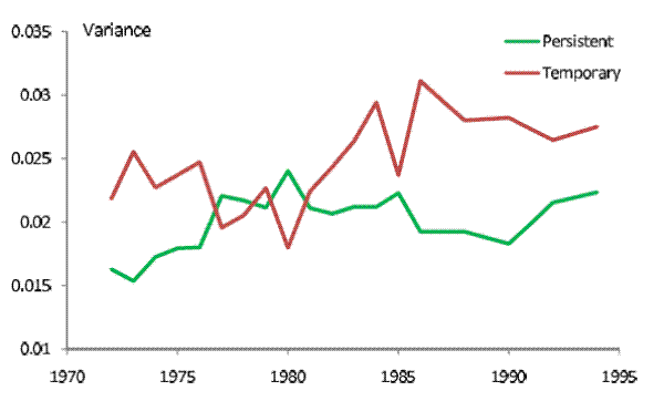
The calibration result suggests that $\rho = 0.91$ , while Figure 9 plots the variances $\sigma^2_{p}$ and $\sigma^2_{z}$ for this calibration. Consistent with most studies, we find that the persistent shocks have a smaller variance (on an annual basis) than the temporary shocks. The variance of the persistent shocks averages to 0.020 while the standard deviation of the temporary shocks averages to 0.025. Both time series trend upward, albeit noisily, with a net increase of 37% (from 0.016 to 0.022) for the persistent shocks and of 26% (from 0.022 to 0.028) for the temporary shocks. The variability of the persistent shocks increased sharply during the 70s, fell off slightly during the 80s, and then rebounded in the 90s. The temporary shocks lost variability during the 70s, saw a sharp increase in the early 80s, and declined marginally afterwards.

7 Precautionary Saving

Finally, to assess the quantitative importance of the changes in income uncertainty on household behavior, we consider how aggregate saving would change in a stylized general-equilibrium model based on Aiyagari (1994).¹⁸ Specifically, we compare the level of precautionary savings implied by the 1972 level of income uncertainty and the 1994 level of income uncertainty.

A continuum of infinitely-lived households of unit measure maximize expected utility

$\displaystyle E\left[ \sum_{t=0}^{\infty }\beta ^{t}u(c_{t};\gamma )\right] ,$

(12)

where $\beta \in (0,1)$ and $u(c;\gamma )$ is CRRA utility

$\displaystyle u(c;\gamma )=\left\{ \begin{array}{cc} \frac{1}{1-\gamma }c^{1-\gamma } & \gamma \neq 1 \\ \ln c & \gamma =1 \end{array} \right. .$

(13)

Each household enjoys an idiosyncratic, uninsurable stream of labor productivity $l_{t}\in \{L_{1},...,L_{m}\}$ , where $0\leq L_{1}<L_{2}<\cdots <L_{m}$ , which can be sold in the labor market for the real wage

. The household's income is a Markov process with transition matrix

$\displaystyle \Pr [l_{t+1}=L_{j}\vert l_{t}=L_{i}]=\pi _{ij}$ .

(14)

There is one risk-free asset that pays gross interest

. Thus the Bellman equation for a household in this economy can be written

$\displaystyle v(x_{t},l_{t})=\max_{0\leq c_{t}\leq x_{t}+\frac{wL_{1}}{r}}u(c_{t})+\beta E[v(wl_{t+1}+R(x_{t}-c_{t}),l_{t+1})\vert l_{t}],$

(15)

where cash on hand $x_{t}$ is the sum of current income and financial wealth, and

is the net interest rate.¹⁹

To close the model, we assume there is a production sector with the Cobb-Douglas production function

$\displaystyle Y=K^{\alpha }N^{1-\alpha },$

(16)

where

is the capital stock and

is the supply of labor. Capital depreciates at the rate $\delta$ . Prices are determined by the profit-maximizing conditions

$\displaystyle R=\alpha K^{\alpha -1}+1-\delta$

(17)

and

$\displaystyle w=(1-\alpha )K^{\alpha }N^{-\alpha }.$

(18)

In equilibrium, the labor supply is the average of productivity of workers (since they have unit measure)

$\displaystyle N=E[l]$

(19)

and the capital stock is the average of their demand for assets

$\displaystyle K=E[x-c(x,l)]$ .

(20)

Aggregate consumption is mean consumption

$\displaystyle C=E[c(x,l)]$ .

(21)

To complete the calibration, we set the share of capital to $\alpha =0.34$ . To match the macroeconomic targets and , we set the depreciation rate to $\delta =0.083$ and the discount factor to $\beta =0.965$ . This leaves the risk aversion parameter, which we set to $\gamma =3$ . This is within the range of values typically considered in the literature, and it also works well for matching properties of the lifecycle profile of consumption (Feigenbaum (2008)).

Because the process for cash on hand is highly persistent, a large number of simulations is necessary to achieve sufficient convergence of the sample average. We compute aggregate variables for steady state equilibria using simulations of a representative agent over ten billion periods. The results are given in Table 3 for different choices of $\sigma^2_{p}$ and $\sigma^2_{z}$ . In line 1, we set $\sigma^2_{p} = 0.016$ and $\sigma^2_{z} = 0.022$ , consistent with the estimated income uncertainty at the beginning of the sample period (1972). In line 4, we set $\sigma^2_{p} = 0.022$ and $\sigma^2_{z} = 0.028$ , consistent with the estimated income uncertainty at the end of the sample period (1994). The contrast between lines 1 and 4 informs us of the total changes due to the increases in income uncertainty. To better understand the contribution of the increases in persistent and transitory shocks variances, in lines 2 and 3 respectively, we alter only one of $\sigma^2_{p}$ and $\sigma^2_{z}$ relative to line 1. Thus, the comparison between lines 1 and 2 indicates the net contribution of the increase in persistent shock variance, while the comparison between lines 1 and 3 shows the effects of greater transitory shock variances.

We focus on aggregate precautionary saving, the portion $K^{PS}$ of the capital stock that would not arise in the corresponding model without uncertainty, i.e. where $\sigma^2_{p} = \sigma^2_{z} = 0$ . Contrasting lines 1 and 4, we find that the steady state level of capital stock due to precautionary saving increases from 0.440 when income uncertainty is low to 0.586 when income uncertainty is high, a 33% increase. Comparing line 1 with lines 2 and 3 respectively, we notice that the increase in the variance of persistent shocks alone accounts for 32 percentage points of the increase, while the increase in the variance of transitory income shocks alone would contribute only a fraction of a percentage point. Thus it is really only the change in the persistent shock that will impact consumer behavior in the aggregate.

The increase in the total capital stock, , along with the other macroeconomic variables and is small relative to the increase in income uncertainty because only the saving for precautionary motives responds to changes in uncertainties, and precautionary saving only accounts for a small fraction of the total saving.

Table 3: Aggregate Variables for Steady-state Equilibria.
	$\sigma^2_{p}$	$\sigma^2_{z}$	$K^{PS}$
(1) 1972 calibration	0.016	0.022	0.440	4.918	1.712	1.302	3.413%
(2) higher $\sigma^2_z$ only	0.016	0.028	0.442	4.920	1.712	1.302	3.411%
(3) higher $\sigma^2_p$ only	0.022	0.022	0.582	5.060	1.728	1.307	3.195%
(4) 1994 calibration	0.022	0.028	0.585	5.063	1.729	1.307	3.190%

Notes: $\sigma^2_p$ and $\sigma^2_z$ denote the variance of persistent and transitory shocks, respectively. $K^{PS}$ denotes the capital stock due to precautionary reasons.

8 Concluding Remarks

This paper documents a substantial increase in household income uncertainties during the last three decades. Our approach does not impose any restrictions on the statistical properties of the underlying income shocks. In addition, the unpredictable component of future income is estimated using only the information available to households when expectations are formed. In contrast to the dramatic decline in the volatility of output growth observed in aggregate data, household income uncertainty, estimated as the variance of forecast errors, exhibited a large increase from the early 1970s to the early 2000s. For example, near term family non-capital income uncertainty rose by 40 percent. The rise is observed for various income measures across time and for all subpopulations. However, some groups that historically enjoyed lower levels of income uncertainty, such as the high-income households, experienced the largest percentage increase.

Solving a general-equilibrium consumption optimization model we find that such an increase in income uncertainty would call for precautionary saving to increase by more than 30 percent and aggregate capital stock to increase by 3 percent. These results are somewhat counterfactual because the personal saving rate in the U.S. has, on net, declined over the same period. Two factors potentially account for the discrepancy between what the model predicts and what is observed in data. First, social insurance may have improved during this period, reducing the precautionary motive for saving (Krueger and Perri (2001)). Second, households may have underestimated the income uncertainty and consequently have saved less than the optimal amount. Quantifying the roles played by these factors is the next topic on our research agenda.

Bibliography

Aiyagari, S. Rao, (1994),

"Uninsured Idiosyncratic Risk and Aggregate Saving," Quarterly Journal of Economics, 109(3), pp. 659-684.

Baker, Michael, and Gary Solon, (2003),

"Earnings Dynamics and Inequality among Canadian Men, 1976-1992: Evidence from Longitudinal Income Tax Records," Journal of Labor Economics, 21(2), pp. 289-321.

Blundell, Richard, Luigi Pistaferri and Ian Preston, (2008) "Consumption Inequality and Partial Insurance." American Economic Review, 98(5): pp., 1887

-1921.

Campbell, John, Martin Lettau, Burton Malkiel, and Yexiao Xu, (2001)

"Have Individual Stocks Become More Volatile? An Empirical Exploration of Idiosyncratic Risk" , Journal of Finance 56(1): pp. 1-43.

Campbell, Sean, (2007)

"Macroeconomic Volatility, Predictability and Uncertainty in the Great Moderation: Evidence from the Survey of Professional Forecasters," Journal of Business and Economic Statistics 25(2): pp. 191-200.

Carroll, Christopher D., and Andrew A. Samwick, (1997),

"The Nature of Precautionary Wealth," Journal of Monetary Economics, 40(1), pp. 41-71.

Carroll, Christopher D. and Andrew A. Samwick, (1998),

"How Important is Precautionary Saving?" Review of Economics and Statistics 80(3), pp. 410-419.

Comin, Diego and Thomas Philippon, (2005),

"The Rise in Firm-Level Volatility: Causes and Consequences", NBER Macroeconomics Annual 20, pp. 167-201.

Cunha, Flavio, James Heckman, and Salvador Navarro, (2005),

"Separating Uncertainty from Heterogeneity in Life Cycle Earnings," Oxford Economic Papers, 57(2), pp. 191-261.

Dynan, Karen, Douglas W. Elmendorf, and Daniel E. Sichel, (2006a),

"Financial Innovation and the Great Moderation: What Do HOusehold Data Say?" Working Paper.

Dynan, Karen, Douglas W. Elmendorf and Daniel E. Sichel, (2007),

"The Evolution of Household Income Volatility," Federal Reserve Board Finance and Economics Discussion Series, 2007

-61.

Feigenbaum, James, (2008),

"Precautionary Saving Unfettered," Working Paper.

Feigenbaum, James and Geng Li, (2011),

"Lifecycle Dynamics of Income Uncertainty and Consumption" , Working Paper.

Gorbachev, Olga, (2010),

"Did Household Consumption Become More Volatile?" American Economic Review forthcoming.

Gottschalk, Peter and Robert Moffitt, (2009)

"The Rising Instability of U.S. Earnings," Journal of Economic Perspectives, 23(4), pp. 3-24.

Gourinchas, Pierre-Olivier and Jonathan A. Parker, (2002),

"Consumption over the Life Cycle," Econometrica 70(1), pp. 47-89.

Guvenen, Fatih, and Anthony Smith, (2008),

"Inferring Labor Income Risk from Economic Choices: An Indirect Inference Approach," working paper.

Jensen, Shane and Stephen Shore, (2010)

"Semi-Parametric Bayesian Modelling of Income Volatility Heterogeneity and Dynamics," working paper.

Keys, Benjamin, (2008)

"Trends in Income and Consumption Volatility, 1970-2000," in Income Volatility and Food Assistance in the United States, Dean Jolliffe and James P. Ziliak, eds. W.E. Upjohn Institute for Employment Research, Kalamazoo, MI.

Kim, Chang-Jin and Charles Nelson, (1999),

"Has the U.S. Economy Become More Stable? A Bayesian Approach Based on a Markov-Switching Model of the Business Cycle," Review of Economics and Statistics 81(4), pp. 608-616.

McConnell, Margaret and Perez-Quiros, Gabriel, (2000),

"Output Fluctuations in the U.S.: What Has Changed Since the Early 1980s?" American Economic Review 90(5), pp. 1464-1476.

Moffitt, Robert and Peter Gottschalk, (2008)

"Trends in the Transitory Variance of Male Earnings in the U.S., 1970-2004", working paper.

Pesaran, Hashem, (2006),

"Multiple Structural Breaks, Forecasting and Present Value Calculations," Computing in Economics and Finance Conference.

Solon, Gary and Donggyun Shin, (2010),

"Trends in Mens Earnings Volatility: What Does the Panel Study of Income Dynamics Show?" Journal of Public Economics, forthcoming.

Stock, James and Mark Watson, (2002),

"Has the Business Cycle Changed and Why?" NBER Macroeconomics Annual 159-218.

Figure 1: Trends in family non-capital income uncertainty

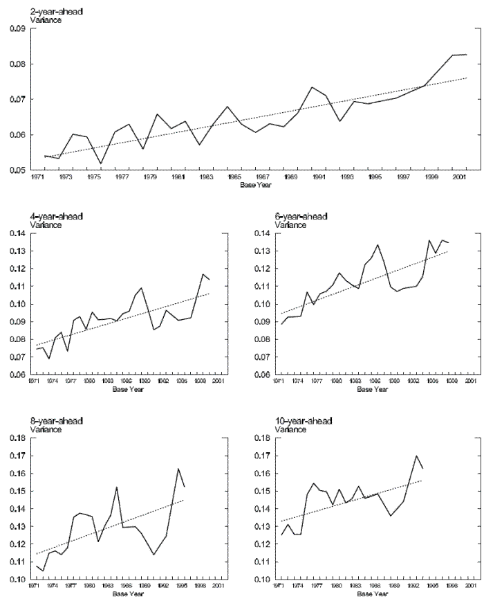
Note: Income uncertainty is measured as the cross-sectional variances of the forecast errors in Eq. (4) in the text.

Accessible Version

Figure 2: Trends in the persistence of forecast errors

Figure 2. Trends in the persistence of forecast errors. Link to accessible version follows.

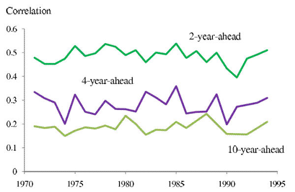
Note: The three series are the coefficients of correlation, estimated in each year from 1971 to 1994, between the 1-year-ahead forecast errors and the 2-, 4-, and 10-year ahead forecast errors, respectively. The correlations between the 1-year-ahead forecast errors and the forecast errors at other horizons (not shown) also remained stable during this period.

Accessible Version

Figure 3: Comparing the income uncertainty profiles in 1970s and 2000s

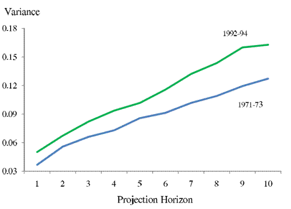
Note: The upper curve shows the average of the family non-capital income uncertainty profile of all horizons ( = 1 - 10) estimated for years 1992, 93, and 94. The lower curve shows the average of the family non-capital income uncertainty profile of all horizons ( = 1 - 10) estimated for year 1992, 93, and 94. Comparing the two curves, we see the growth of forecast errors' variances is greater at farther horizons than at nearer horizons, suggesting that the variance of persistent income shocks had increased during this period.

Accessible Version

Figure 4: Income uncertainty of single-earners and dual-earners

Figure 4. Income uncertainty of single-earners and dual-earners. Link to accessible version follows.

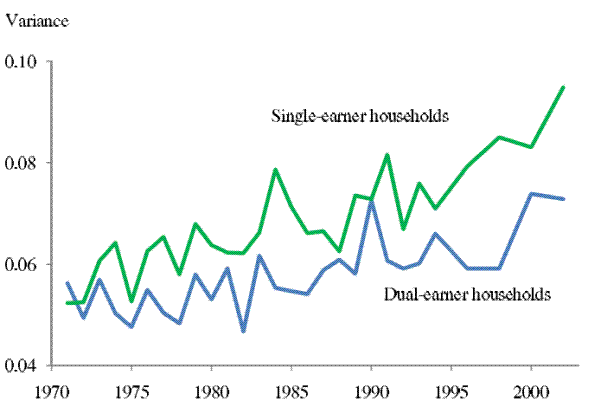
Note: The two series plot the 2-year-ahead income uncertainty for single-earner and dual-earner households, respectively. Dual-earner households are defined as those for which wife's labor earnings is greater than 25% of the head's labor earnings in the base year.

Accessible Version

Figure 5: Income uncertainty across income quartiles

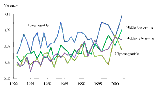
Note: The four series plot the 2-year-ahead income uncertainty for the households in each income quartile, respectively. Income quartile is defined according to the average family non-capital income in year , , and .

Accessible Version

Figure 6: Income uncertainty estimated using samples created with different trimming thresholds

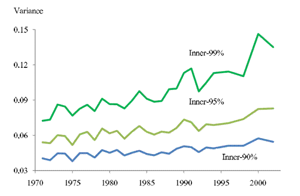
Note: The top curve plots the 2-year-ahead income uncertainty across years using a sample constructed after trimming off the top and bottom 0.5% of the distribution of income growth between and . The middle curve replicates the curve in the top panel in Figure 1. The bottom curve plots the 2-year-ahead income uncertainty across years using a sample constructed after trimming off the top and bottom 5% of the distribution of income growth between and .

Accessible Version

Figure 7: Income uncertainty estimated using an invariant sample

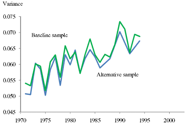
Note: The upper curve replicates the curve in the top panel in Figure 1. The lower curve is the 2-year-ahead income uncertainty series estimated using a sample of households that are in the sample for estimating eq. (4) for = 10.

Accessible Version

Figure 8: Income uncertainty estimated with additional information

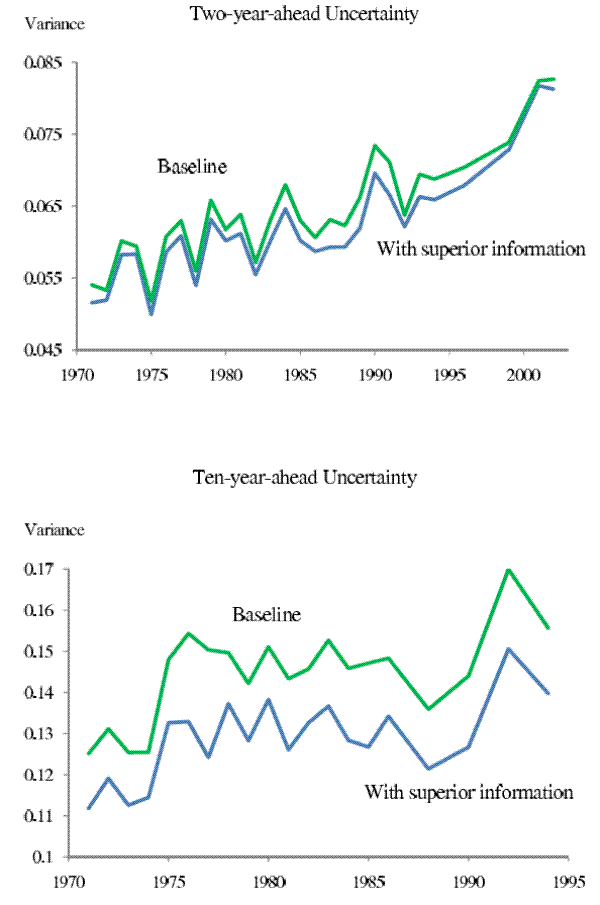
Note: The upper curve in the top panel replicates the curve in the top panel in Figure 1. The lower curve in the top panel is the 2-year-ahead income uncertainty series estimated assuming that the households in year know their family size, marital status, industry and occupation in year . The upper curve in the bottom panel replicates the curve in the bottom-right panel in Figure 1. The lower curve in the top panel is the 10-year-ahead income uncertainty series estimated assuming that the households in year know their family size, marital status, industry and occupation in year .

Accessible Version

Figure 9: Trends of Persistent and Transitory Income Shock Variances

Figure 9. Trends of Persistent and Transitory Income Shock Variances. Link to accessible version follows.

Accessible Version

Footnotes

* Department of Economics and Finance; Utah State University; Logan, UT 84322-3565. E-mail: [email protected].edu. Return to Text

** Federal Reserve Board, Mail Stop 93, Washington, DC 20551. E-mail: [email protected]. The views presented in this paper are those of the authors and are not necessarily those of the Federal Reserve Board or its staff.
For helpful comments, we thank Karen Dynan, Michael Palumbo, and seminar participants at the Econometric Society North American Summer Meetings, the Federal Reserve Board, Midwest Macro Meetings, NBER Summer Institute, and the Society of Economic Dynamics Annual Meetings. All remaining errors are our own. Return to Text

1. McConnell and Perez-Quiros (2000) adopt a classical linear framework, whereas Kim and Nelson (1999) use a Bayesian approach. Return to Text

2. Heightened volatilities at the household level can also be found in consumption data. Gorbachev (2010) documents that household consumption volatility, after controlling for predictable movements in interest rates, preferences and income shocks, rose noticeably between the early 1970s and early 2000s. Moreover, out of the household sector, other evidence of increased micro-level volatilities include Campbell et al. (2001) and Comin and Pilippon (2005). The former finds that since the early 1960s to the late 1990s, whereas market-level stock-return volatilities have become quite stable, especially during the Great Moderation era, there has been a noticeable increase in firm-level stock volatility relative to the market volatility. The latter paper shows that the decline in aggregate volatility was accompanied by a large increase in firm-level volatility in other measures such as sales, employment, and capital expenditure. Return to Text

3. We use the double subscript

instead of

to remind us that income uncertainty can vary with both

and

separately, not only with

. Return to Text

4. We refer the readers to the cited paper for more details about the model and how it compares to other models in the literature. Return to Text

5. We use a fourth-order polynomial of age evaluated at time

because age is not stochastic. Return to Text

6. Also, according to the PSID staff, the individual response rate in 2005, adjusted for known mortality, among the original sample members, i.e. those in the study in 1968, was about 34.5%, which roughly speaking implies an attrition rate lower than 3%. Return to Text

7. Before 1979, head labor earning is the sum of the following components: labor part of farm income, labor part of roomers and boarders income, labor part of business income, wages, bonuses, overtime income, commissions income and professional practice income. Each component is collected in the survey. Labor part of market gardening income was added in 1979, income from extra job was added in 1993, but labor part of farm, business and roomers and borders income were excluded from 1994 because the PSID no longer asks for this information separately. Likewise, wife labor earnings details also changed substantially across waves. Despite these variations in the survey, we do not make additional adjustments with respect to labor income because the labor earning components other than the head salaries and wages, which has been collected consistently after 1969, are relatively small. Second, many of the minor components were masked into brackets in earlier waves. Return to Text

8. The PSID does not separate labor income from taxable income of other family members in most of the waves. Return to Text

9. We include households with various tenures of participation without restriction to construct a balanced panel because we want to retain a sample as large as possible as long as the sample is capable of estimating Equation (4). Later we will show that our results are robust in a subsample that is a balanced panel. Return to Text

10. Our trimming technique risks being exceedingly aggressive if the trimmed observations reflect true income fluctuation instead of measurement errors. Should this be the case, our results reflect the dynamics of income uncertainty for the vast majority of the population. As a robustness check, we will present the trend in income uncertainty estimated using a sample with only the top and bottom one half of one percent of the income growth distribution trimmed off. Return to Text

11. We mindfully choose the sample break year to be close to the break point year identified in Kim and Nelson (1999) and McConnell and Perez-Quiros (2000) and to have similar number of waves so that the statistics are comparable. Indeed, these two subsamples have the same number of waves of data as the PSID became biennial after 1997. Return to Text

12. It is worthwhile to point out that the PSID aggregate income measures are constructed without using weights. When weights are used, the volatility moderation becomes less pronounced. This is likely due to the fact that PSID weights are not calculated to match aggregate income. In addition, we use the PSID mean income growth and therefore do not take into account the underlying population growth. Return to Text

13. We plot the even-number future horizons because these series have longer time series than the series of odd-number future horizons. We linearly interpolate the series for the years of 1997, 1999, and 2001 when applicable. Return to Text

14. Feigenbaum and Li (2011) show strong evidence that the persistent component of the income shocks either does not contain a unit root process or contains such a process with innovations of small variances. Return to Text

15. Some work on time-consistent rational-expectations models of structural breaks has been done, for example by Pesaran (2006), but this is a quite recent field of research. Return to Text

16. For simplicity, we assume there is no deterministic trend in income. Return to Text

17. The loss function actually depends on the standard deviations rather than the variances, so the elements of both matrices are of comparable size. Return to Text

18. We could alternatively solve for the change in aggregate saving in a partial-equilibrium model where

is constant. However, as Huggett (1993) and Aiyagari (1994) emphasized, this will exaggerate the apparent behavioral change. Return to Text

19. Note that the upper bound on consumption follows if we impose a no-Ponzi game condition. The most a household can borrow and be sure that it can repay its debt is $wL_{1}/r$ (Aiyagari (1994)). Return to Text

^♣ This version is optimized for use by screen readers. Descriptions for all mathematical expressions are provided in LaTex format. A printable pdf version is available. Return to Text