
Stock Return Predictability and Variance Risk Premia: Statistical Inference and International Evidence *
Keywords: Variance risk premium; return predictability; over-lapping return regressions; international stock market returns; global variance risk.
Abstract:
Recent empirical evidence suggests that the variance risk premium, or the difference between risk-neutral and statistical expectations of the future return variation, predicts aggregate stock market returns, with the predictability especially strong at the 2-4 month horizons. We provide extensive Monte Carlo simulation evidence that statistical finite sample biases in the overlapping return regressions underlying these findings can not "explain" this apparent predictability. Further corroborating the existing empirical evidence, we show that the patterns in the predictability across different return horizons estimated from country specific regressions for France, Germany, Japan, Switzerland and the U.K. are remarkably similar to the pattern previously documented for the U.S. Defining a "global" variance risk premium, we uncover even stronger predictability and almost identical cross-country patterns through the use of panel regressions that effectively restrict the compensation for world-wide variance risk to be the same across countries. Our findings are broadly consistent with the implications from a stylized two-country general equilibrium model explicitly incorporating the effects of world-wide time-varying economic uncertainty.
1 Introduction
A number of recent studies have suggested that aggregate U.S. stock market return is predictable over horizons ranging up to a few quarters based on the difference between options-implied and actual realized variation measures, or the so-called variance risk premium (see, e.g., Zhou, 2010; Bollerslev, Tauchen, and Zhou, 2009; Drechsler and Yaron, 2011; Gabaix, 2011; Zhou and Zhu, 2009; Kelly, 2011, among others). These findings of apparent predictability over relatively short quarterly horizons have potentially far reaching implications for many issues in asset pricing finance. They are also distinctly different from the longer-run multi-year return predictability patterns that have been studied extensively in the existing literature, in which the predictability is typically associated with more traditional valuation measures such as dividend yields, P/E ratios, or consumption-wealth ratios (see, e.g., Campbell and Shiller, 1988b; Lettau and Ludvigson, 2001; Fama and French, 1988, among others). Motivated by these observations, the main goal of the present paper is to further examine the robustness and the scope of these striking new empirical findings.
Our investigations are essentially twofold. First, to assess the validity of the statistical inference procedures underlying the empirical findings, we report the results from an extensive Monte Carlo simulation exercise designed to closely mimic the dynamic dependencies inherent in daily returns and variance risk premia. Our results clearly suggest that statistical biases can not "explain" the documented return predictability patterns. At the same time, the results also suggest that the use of finer sampled observations, say daily as opposed to monthly data as employed in the above cited studies, provides limited additional power to detect the predictability inherent in the variance risk premium.
Second, in a separate effort to expand on and corroborate the existing empirical evidence pertaining to monthly U.S. returns, we extend the same basic ideas and regressions to several other countries. In so doing, we also define a "global" variance risk premium. We show that this simple aggregate measure of world-wide economic uncertainty results in even stronger predictability for all of the countries in the sample. We also show that these new empirical findings are broadly consistent with the implications from a stylized two-country general equilibrium model that explicitly incorporates the effect of time-varying economic uncertainty across countries.
The finite sample properties of overlapping long-horizon return regressions have been studied extensively in the existing literature. Boudoukh, Richardson, and Whitelaw (2008), for instance, have recently shown that even in the absence of any increase in the true predictability, the values of the
![]() 's in regressions involving highly persistent predictor variables and overlapping returns will by construction increase roughly proportional to the return horizon and the length of the
overlap.6 In line with the procedures adapted in the existing literature, we will focus on the Newey and
West (1987) and Hodrick (1992)
type
's in regressions involving highly persistent predictor variables and overlapping returns will by construction increase roughly proportional to the return horizon and the length of the
overlap.6 In line with the procedures adapted in the existing literature, we will focus on the Newey and
West (1987) and Hodrick (1992)
type ![]() -statistics. Both of these are robust asymptotically to heteroskedasticity and serial correlation in the residuals from the estimated regressions. Our simulation design is based on an
empirically realistic bivariate VAR-GARCH-DCC model for the joint daily return and variance risk premium dynamics. We find both of the
-statistics. Both of these are robust asymptotically to heteroskedasticity and serial correlation in the residuals from the estimated regressions. Our simulation design is based on an
empirically realistic bivariate VAR-GARCH-DCC model for the joint daily return and variance risk premium dynamics. We find both of the ![]() -statistics to be reasonably well behaved, albeit
slightly over-sized under the null hypothesis of no predictability. We also find that the Newey-West based
-statistics to be reasonably well behaved, albeit
slightly over-sized under the null hypothesis of no predictability. We also find that the Newey-West based ![]() -statistics result in marginally more powerful (size adjusted) tests under the
alternative. Moreover, directly in line with the results in the existing literature on long-horizon return predictability, the quantiles in the finite sample distribution of the
-statistics result in marginally more powerful (size adjusted) tests under the
alternative. Moreover, directly in line with the results in the existing literature on long-horizon return predictability, the quantiles in the finite sample distribution of the ![]() 's from the
regressions are spuriously increasing with the return horizon under the null of no predictability.7 At the same time, the
's from the
regressions are spuriously increasing with the return horizon under the null of no predictability.7 At the same time, the ![]() 's implied by the daily VAR-GARCH-DCC model exhibit a distinct hump shape in the degree of predictability that closely mimics the pattern actually observed in U.S. return regressions.
's implied by the daily VAR-GARCH-DCC model exhibit a distinct hump shape in the degree of predictability that closely mimics the pattern actually observed in U.S. return regressions.
Guided by the Monte Carlo simulations, we rely on the Newey-West based ![]() -statistics and monthly return regressions to summarize our new international evidence. Due to data availability and
the required liquidity of options markets, we restrict our attention to the six major financial markets of France, Germany, Japan, Switzerland, the U.K., and the U.S. Our empirical result shows that the country specific regressions based on regressing each country's return on its own variance risk
premium result in similar hump-shaped regression coefficients and
-statistics and monthly return regressions to summarize our new international evidence. Due to data availability and
the required liquidity of options markets, we restrict our attention to the six major financial markets of France, Germany, Japan, Switzerland, the U.K., and the U.S. Our empirical result shows that the country specific regressions based on regressing each country's return on its own variance risk
premium result in similar hump-shaped regression coefficients and ![]() 's for all of the six countries. However, the degree of predictability afforded by the country specific variance risk
premia and the statistical significance of the results generally are not as strong as the previously reported results for the U.S. market.
's for all of the six countries. However, the degree of predictability afforded by the country specific variance risk
premia and the statistical significance of the results generally are not as strong as the previously reported results for the U.S. market.
These results naturally point to the possibility of world-wide variance risk, as opposed to the country specific variance risk premia, being priced. To investigate this idea, we construct a "global" variance risk premium, defined as a simple market capitalization weighted average of the individual country variance risk premia. Restricting the effect on this "global" variance risk premium to be the same across countries in a panel return regression results in much stronger findings for all of the countries, with a uniform peak in the degree of predictability at the four month horizons. Moreover, the degree of predictability afforded by this "global" variance risk premium easily exceeds that of the implied and realized variation measures when included in isolation. It also clearly dominates that of other traditional predictor variables that have been shown to work well over longer annual horizons, including the P/E ratio. While this new international evidence indirectly corroborates the previous findings based exclusively on U.S. data reported in the studies cited above, importantly the results also point to the existence of even stronger predictability through the use of alternative definitions of world-wide variance risk.8
Our new empirical findings are, of course, related to the large existing literature on international stock return predictability (see, e.g., Harvey, 1991; Bekaert and Hodrick, 1992; Ferson and Harvey, 1993; Campbell and Hamao, 1992, among others). However, the focus of this literature has traditionally been on longer-run multi-year return predictability. By contrast, our results pertaining to the "global" variance risk premium concern much shorter-run within year predictability, and are essentially "orthogonal" to the findings reported in the existing literature.9 At the same time, however, the new empirical results are generally in line with the calibrations from a simple theoretical two-country model that explicitly incorporates the equilibrium effects of time-varying economic uncertainty across countries.
The rest of the paper is organized as follows. Section 2 presents our Monte Carlo based simulation evidence pertaining to the statistical inference procedures underlying the existing empirical findings. Section 3 discusses our new international evidence and the results for our "global" variance risk premia measure, along with our equilibrium model based calibrations. Section 4 concludes.
2. General Setup and Monte Carlo Simulations
The key empirical findings reported in Bollerslev, Tauchen, and Zhou (2009) (BTZ2009, henceforth), and the subsequent studies cited above, are based on simple OLS regressions of the returns on the aggregate market portfolio over monthly and longer return horizons on a measure of the one-month variance
risk premium. In particular, let
![]() and
and ![]() denote the continuously compounded return from time
denote the continuously compounded return from time
![]() to time
to time ![]() and the variance risk premium at time
and the variance risk premium at time ![]() , respectively. Defining the unit time interval to be one trading day, the multi-period return regressions in BTZ2009 may then be expressed as special cases of,
, respectively. Defining the unit time interval to be one trading day, the multi-period return regressions in BTZ2009 may then be expressed as special cases of,
 |
(1) |
for
Meanwhile, it is well known that in the context of overlapping return observations, the regression in (1) can result in spuriously large and highly misleading regression ![]() 's, say
's, say
![]() , as the horizon
, as the horizon ![]() increases; see, e.g., the discussion and many references
in Campbell, Lo, and MacKinlay (1997). Similarly, the standard errors for the OLS estimates designed to take account of the serial correlation in
increases; see, e.g., the discussion and many references
in Campbell, Lo, and MacKinlay (1997). Similarly, the standard errors for the OLS estimates designed to take account of the serial correlation in
![]() based on the Bartlett kernel advocated by () (NW, henceforth), and the modification proposed by Hodrick (1992) (HD, henceforth), can
also both result in
based on the Bartlett kernel advocated by () (NW, henceforth), and the modification proposed by Hodrick (1992) (HD, henceforth), can
also both result in ![]() -statistics for testing hypotheses about
-statistics for testing hypotheses about ![]() and
and
![]() that are poorly approximated by a standard normal distribution. Most of the existing analyses pertaining to these and other related finite sample biases, however, have been
calibrated to situations with a highly persistent predictor variable, as traditionally used in long-horizon return regressions. Even though the variance risk premium is fairly persistent at the daily frequency, it is much less so at the monthly level, and as such one might naturally expect the
finite sample biases to be less severe in this situation.10 Our Monte Carlo simulations discussed in the next section confirm this conjecture in an
empirically realistic setting designed to closely mimic the joint dependencies in actual daily returns and variance risk premia.
that are poorly approximated by a standard normal distribution. Most of the existing analyses pertaining to these and other related finite sample biases, however, have been
calibrated to situations with a highly persistent predictor variable, as traditionally used in long-horizon return regressions. Even though the variance risk premium is fairly persistent at the daily frequency, it is much less so at the monthly level, and as such one might naturally expect the
finite sample biases to be less severe in this situation.10 Our Monte Carlo simulations discussed in the next section confirm this conjecture in an
empirically realistic setting designed to closely mimic the joint dependencies in actual daily returns and variance risk premia.
2.1 Simulation Design
The model underlying our simulations is based on daily S![]() P500 composite index returns (obtained from CRSP). The corresponding daily observations on the variance risk
premium are defined as
P500 composite index returns (obtained from CRSP). The corresponding daily observations on the variance risk
premium are defined as
![]() , where we rely on the square of the new VIX index (obtained from the CBOE) to quantify the implied variation
, where we rely on the square of the new VIX index (obtained from the CBOE) to quantify the implied variation ![]() , and the summation of current and previous 20 trading days daily realized variances (obtained from the Oxford-Man Institute's Realized Volatility Library) together with the squared overnight returns to quantify the total realized
variation over the previous month
, and the summation of current and previous 20 trading days daily realized variances (obtained from the Oxford-Man Institute's Realized Volatility Library) together with the squared overnight returns to quantify the total realized
variation over the previous month
![]() .11 The span of the data runs from
February 1, 1996 to December 31, 2007, for a total of 2,954 daily observations.
.11 The span of the data runs from
February 1, 1996 to December 31, 2007, for a total of 2,954 daily observations.
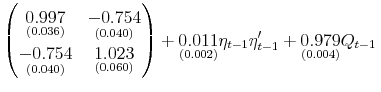
After some experimentation, we arrived at the following bivariate VAR (1)-GARCH![]() -DCC model (see Engle, 2002 , for additional details on the DCC model) for the two daily time series,
-DCC model (see Engle, 2002 , for additional details on the DCC model) for the two daily time series,
where
The model implies a strong negative (on average) correlation between the innovations to the return and VRP equations. This, of course, is consistent with the well documented "leverage" effect; see, e.g., Bollerslev, Sizova, and Tauchen (2011) and the many references therein. At the same time, as is
evident from the equation for ![]() , and the corresponding plot in the top panel in Figure 1, the value of the conditional correlation clearly varies over time, reaching a low of close to -0.85 toward the end of the sample. The bottom three panels in Figure 1 indicate that the distribution of the estimated standardized residuals from the model (i.e.,
, and the corresponding plot in the top panel in Figure 1, the value of the conditional correlation clearly varies over time, reaching a low of close to -0.85 toward the end of the sample. The bottom three panels in Figure 1 indicate that the distribution of the estimated standardized residuals from the model (i.e.,
![]() , where
, where
![]() =
=
![]() ) are well behaved and centered at zero, with variances close to unity, albeit not normally distributed.12 All in all, however, the model provides a reasonably good fit to the joint dynamic dependencies inherent in the two daily series.
) are well behaved and centered at zero, with variances close to unity, albeit not normally distributed.12 All in all, however, the model provides a reasonably good fit to the joint dynamic dependencies inherent in the two daily series.
As such, we will use this relatively simple-to-implement model as our basic data generating process for the Monte Carlo simulations, and our analysis of the finite sample properties of the NW and HD ![]() -statistics, and
-statistics, and ![]() 's from the overlapping return regressions in equation (1).13 Our simulated finite sample distributions will be based on a total of 2,000 bootstrapped replications from the model. We will look at sample frequencies of
's from the overlapping return regressions in equation (1).13 Our simulated finite sample distributions will be based on a total of 2,000 bootstrapped replications from the model. We will look at sample frequencies of
![]() "daily"
"daily"![]() ,
,
![]() "weekly"
"weekly"![]() and
and
![]() "monthly"
"monthly"![]() , and return horizons
, and return horizons ![]() ranging up to 240 "days," or 12 "months." The number of observations for each of the simulated samples is fixed at
ranging up to 240 "days," or 12 "months." The number of observations for each of the simulated samples is fixed at ![]() "days" (or 598
"weeks," or 149 "months"), corresponding to the length of the actual sample used in the estimation of the VAR-GARCH-DCC model above. We begin with a discussion of the size and power properties of the two
"days" (or 598
"weeks," or 149 "months"), corresponding to the length of the actual sample used in the estimation of the VAR-GARCH-DCC model above. We begin with a discussion of the size and power properties of the two ![]() -statistics.
-statistics.
2.2 Size and Power
Our characterization of the distributions under the null hypothesis of no return predictability is based on restricting the coefficients associated with
![]() and
and ![]() in the return equation to be identically equal to zero,
leaving all of the other coefficients at their estimated values. Table 1 reports the resulting simulated the 95th percentiles of the
in the return equation to be identically equal to zero,
leaving all of the other coefficients at their estimated values. Table 1 reports the resulting simulated the 95th percentiles of the ![]() and
and ![]() test statistics, along with the regression
test statistics, along with the regression ![]() 's. Directly in line with the evidence in the existing literature, both of the
's. Directly in line with the evidence in the existing literature, both of the ![]() -statistics exhibit non-trivial size distortions relative to the
nominal one-side 95-percent critical value of 1.645. Also, the distortions tend to increase with the return horizon
-statistics exhibit non-trivial size distortions relative to the
nominal one-side 95-percent critical value of 1.645. Also, the distortions tend to increase with the return horizon ![]() . Moreover, consistent with the results reported in Hodrick (1992), the biases for the NW based standard error calculations generally exceed those for the HD standard errors, and markedly more so the longer the return horizon.
. Moreover, consistent with the results reported in Hodrick (1992), the biases for the NW based standard error calculations generally exceed those for the HD standard errors, and markedly more so the longer the return horizon.
To more directly illustrate the results, we plot in the three left panels in Figure 2 the simulated 95-percent critical values for ![]() (dashed lines) and
(dashed lines) and ![]() (solid lines) for
(solid lines) for
![]() . We also include in the figure the
. We also include in the figure the ![]() -statistics obtained by running these
same regressions on the actual daily, weekly and monthly data over the February 1996 through December 2007 sample period used in calibrating the simulated model. As the figure shows, the actual
-statistics obtained by running these
same regressions on the actual daily, weekly and monthly data over the February 1996 through December 2007 sample period used in calibrating the simulated model. As the figure shows, the actual ![]() -statistics systematically exceeds the simulated critical values for return horizons in the range of 2 to 3 months. This is true regardless of whether the regressions are based on daily, weekly, or monthly data. Meanwhile, the
-statistics systematically exceeds the simulated critical values for return horizons in the range of 2 to 3 months. This is true regardless of whether the regressions are based on daily, weekly, or monthly data. Meanwhile, the ![]() -statistics generally do not exceed the simulated critical values and accordingly do not support the idea of return predictability.
-statistics generally do not exceed the simulated critical values and accordingly do not support the idea of return predictability.
In order to better understand this discrepancy in the conclusions drawn from the two tests, we report in Table 2 the power of the tests to detect predictability implied by the
unrestricted VAR-GARCH-DCC model. To facilitate comparisons we only report the size-adjusted power for a 5-percent test. Not surprisingly, the power of both tests decrease with the return horizon. At the same time, the power of the ![]() test systematically exceed that of the
test systematically exceed that of the ![]() test for return horizons less than a year, and the differences appear most pronounced at the
2-4 month horizons.
test for return horizons less than a year, and the differences appear most pronounced at the
2-4 month horizons.
These differences are also evident in the three right panels in Figure 2, which plot the relevant power curves. Comparing the simulations across the three different panels
in the table and the figure also point to fairly small loses in terms of power when decreasing the sampling frequency of the data used in the regressions from
![]() "daily"
"daily"![]() to
to
![]() "weekly"
"weekly"![]() to
to
![]() "monthly"
"monthly"![]() .
.
Guided by these findings we will base our subsequent empirical investigations on the most commonly used monthly return regressions and NW-based standard errors, recognizing that the finite sample distributions of the ![]() -statistics tend to be slightly upward biased under the null of no predictability.
-statistics tend to be slightly upward biased under the null of no predictability.
2.3 
In addition to the ![]() -statistics associated with the
-statistics associated with the ![]() coefficients, the
coefficients, the
![]() 's from the return regressions are often used to assess the strength of the relationship and the effectiveness of the predictor variable across different horizons. Of course, as
previously noted above, it is well known that the biases exhibited by the
's from the return regressions are often used to assess the strength of the relationship and the effectiveness of the predictor variable across different horizons. Of course, as
previously noted above, it is well known that the biases exhibited by the ![]() -statistics in the context of long-horizon return regressions carry over to the
-statistics in the context of long-horizon return regressions carry over to the ![]() 's, and that these need to be carefully interpreted in the context of persistent predictor variables (see, e.g., the aforementioned study by Boudoukh, Richardson, and Whitelaw. 2008, for a recent analysis, along with the many
references therein).
's, and that these need to be carefully interpreted in the context of persistent predictor variables (see, e.g., the aforementioned study by Boudoukh, Richardson, and Whitelaw. 2008, for a recent analysis, along with the many
references therein).
The corresponding columns in Table 1 show that, while less dramatic than the biases over multi-year return horizons, the ![]() 's may still be quite different from zero under the null of no predictability in the present setting. In particular, the 95th percentiles are around 5-6 percent at the 2-4 months horizon for all of the three sampling frequencies
's may still be quite different from zero under the null of no predictability in the present setting. In particular, the 95th percentiles are around 5-6 percent at the 2-4 months horizon for all of the three sampling frequencies
![]() .
.
Further to this effect, we show in the top panel in Figure 3 select quantiles in the simulated distribution of the ![]() 's that obtain in the absence of any predictability. Consistent with the findings in the extant literature pertaining to monthly observations and longer return horizons, all of the quantiles increase monotonically with the return
horizon, and this increase is especially marked for the higher percentiles. Intuitively as the horizon increases, the overlapping return regressions become closer to a spurious type regression.
's that obtain in the absence of any predictability. Consistent with the findings in the extant literature pertaining to monthly observations and longer return horizons, all of the quantiles increase monotonically with the return
horizon, and this increase is especially marked for the higher percentiles. Intuitively as the horizon increases, the overlapping return regressions become closer to a spurious type regression.
In addition to the simulated quantiles, we also include in the same figure the ![]() 's obtained from the actual return regressions based on the same daily data used in estimating the
VAR-GARCH-DCC model. Comparing the actual
's obtained from the actual return regressions based on the same daily data used in estimating the
VAR-GARCH-DCC model. Comparing the actual ![]() 's to the simulated percentiles again suggest that the degree of predictability is most significant at the intermediate 2-4 months horizon.
This, of course, is directly in line with the inference based on the
's to the simulated percentiles again suggest that the degree of predictability is most significant at the intermediate 2-4 months horizon.
This, of course, is directly in line with the inference based on the ![]() -statistics discussed in the previous section, and the prior empirical evidence reported in BTZ2009.
-statistics discussed in the previous section, and the prior empirical evidence reported in BTZ2009.
The hump-shaped pattern in the actual ![]() 's also closely mimics the patterns in the simulated quantiles for the estimated VAR-GARCH-DCC model depicted in the bottom panel in Figure
3. Interestingly, this striking similarity with an apparent peak in the degree of predictability at the intermediate 2-4 months horizon arises in spite of the fact that the
simulated model involves only first-order dynamics in the equations that describe the daily conditional means.
's also closely mimics the patterns in the simulated quantiles for the estimated VAR-GARCH-DCC model depicted in the bottom panel in Figure
3. Interestingly, this striking similarity with an apparent peak in the degree of predictability at the intermediate 2-4 months horizon arises in spite of the fact that the
simulated model involves only first-order dynamics in the equations that describe the daily conditional means.
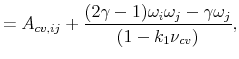
To help understand this result, consider the VAR(1) corresponding to the conditional mean dependencies in the Monte Carlo simulation design,
Following Campbell (2001), it is possible to show that the population regression coefficients and
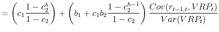 |
||
![\displaystyle =\frac{b(h)^{2}}{h}\frac{Var(VRP_t)}{[h^{-1}Var(\sum_{j=1}^{h}r_{t-1+j,t+j})]}\ .](img71.gif) |
Hence, the strength of the predictability over different horizons
To illustrate this, the solid lines in each of the four panels in Figure 4 show the ![]() 's implied by the unrestricted VAR(1) coefficient estimates used in the simulations. Indirectly confirming the satisfactory fit of the model, the theoretically implied population
's implied by the unrestricted VAR(1) coefficient estimates used in the simulations. Indirectly confirming the satisfactory fit of the model, the theoretically implied population ![]() 's are generally close to the
's are generally close to the ![]() 's actually estimated from the sample regressions depicted by the star-dashed line in the previous Figure 3. Meanwhile, marginally decreasing the value of each of the VAR(1) coefficients,
's actually estimated from the sample regressions depicted by the star-dashed line in the previous Figure 3. Meanwhile, marginally decreasing the value of each of the VAR(1) coefficients, ![]() ,
, ![]() ,
, ![]() and
and ![]() , by ten percent, results in quite different
, by ten percent, results in quite different ![]() 's, as shown by the dashed lines in Figure 4. In particular, the decrease in
's, as shown by the dashed lines in Figure 4. In particular, the decrease in ![]() has by far the largest effect.
Moreover, the value of
has by far the largest effect.
Moreover, the value of ![]() , and the own persistence of
, and the own persistence of ![]() , is intimately linked
to the location of the maximum in the hump shaped predictability pattern.15
, is intimately linked
to the location of the maximum in the hump shaped predictability pattern.15
Taken as a whole, our Monte Carlo simulations and the new regression results based on daily U.S. returns discussed above clearly support the variance risk premium as a powerful predictor at the 2-4 month horizons. At the same time, the overlapping nature of the return regressions tend to attenuate the strength of the predictability somewhat. Hence, in an effort to further corroborate the existing empirical evidence pertaining exclusively to the U.S. market and data prior to the 2008 financial crisis, we next turn to a discussion of our new empirical findings involving more recent data and several other countries.
3 International Evidence
Motivated by the Monte Carlo simulation results in the previous section, we will rely exclusively on the common benchmark monthly sampling frequency, along with the traditional NW-based standard errors and ![]() -statistics, keeping in mind the finite sample biases documented above. We will restrict our analysis to France, Germany, Japan, Switzerland, the U.K., and the U.S., all of which have highly liquid options markets and readily available model-free implied variances for their
respective aggregate market indexes (see , , for a recent summary of the model-free and parametric options implied volatility indexes available for different countries). We begin with a brief discussion of the relevant data.
-statistics, keeping in mind the finite sample biases documented above. We will restrict our analysis to France, Germany, Japan, Switzerland, the U.K., and the U.S., all of which have highly liquid options markets and readily available model-free implied variances for their
respective aggregate market indexes (see , , for a recent summary of the model-free and parametric options implied volatility indexes available for different countries). We begin with a brief discussion of the relevant data.
3.1 Data and Summary Statistics
Our monthly aggregate market index returns are based on daily data for the French CAC 40 (obtained from Euronext), the German DAX 30 (obtained from Deutsche Börse), the Japanese Nikkei 225, the Swiss SMI, and the U.K. FTSE 100 (all obtained from Datastream), and the U.S. S&P 500
(obtained from Standard & Poor's). We use the sum of the daily squared returns over a month to construct end-of-month realized variances ![]() for each of the countries. The
corresponding end-of-month model-free implied volatilities
for each of the countries. The
corresponding end-of-month model-free implied volatilities
![]() for the S&P 500 (VIX) were obtained from the CBOE, the CAC (VCAC) from Euronext, the DAX (VDAX) from Deutsche Börse, while those for the FTSE (VFTSE) and the SMI
(VSMI) were both obtained from Datastream. Our data for the Japanese volatility index (VXJ) is obtained directly from the Center for the Study of Finance and Insurance at Osaka University (see , , for a more detailed discussion of the VXJ index). The sample period for each
of the series extends from January 2000 to December 2010, and as such also allows for an out-of-sample validation of the existing empirical evidence for the U.S. based exclusively on data prior to the recent financial crisis.16
for the S&P 500 (VIX) were obtained from the CBOE, the CAC (VCAC) from Euronext, the DAX (VDAX) from Deutsche Börse, while those for the FTSE (VFTSE) and the SMI
(VSMI) were both obtained from Datastream. Our data for the Japanese volatility index (VXJ) is obtained directly from the Center for the Study of Finance and Insurance at Osaka University (see , , for a more detailed discussion of the VXJ index). The sample period for each
of the series extends from January 2000 to December 2010, and as such also allows for an out-of-sample validation of the existing empirical evidence for the U.S. based exclusively on data prior to the recent financial crisis.16
In accordance with the empirical analysis in the previous section, the variance risk premium for each of the individual countries is simply defined by
![]() . The resulting time series plots in Figure 5 clearly show the dramatic impact of the financial crisis, and the exceptionally large volatility risk premia observed in the Fall of 2008 for all of the countries. Interestingly, the premium for the DAX, and to a lesser extent the SMI, were
almost as large and negative as in 2001-2002.
. The resulting time series plots in Figure 5 clearly show the dramatic impact of the financial crisis, and the exceptionally large volatility risk premia observed in the Fall of 2008 for all of the countries. Interestingly, the premium for the DAX, and to a lesser extent the SMI, were
almost as large and negative as in 2001-2002.
The standard set of summary statistics reported in Table 3 also show a remarkable coherence in the distributions of the variance risk premia and monthly excess returns for each of the countries.17 In particular, looking at Panel A the average excess returns are all negative, ranging from a high of -2.15 for Switzerland to a low of -6.52 for France, reflective of the often-called "lost decade." Of course, the corresponding standard deviations all point to considerable variations in the returns around their sample means.
The variance risk premia are all positive on average, ranging from a low of 4.13 for France to a high of 13.26 for Japan on a percentage-squared monthly basis. "Selling" volatility has been highly profitable on average over the last decade. Meanwhile, consistent with the visual impressions from Figure 5, all of the premia are significantly negatively skewed and exhibit large excess kurtosis. Even though implied and realized variances are both strongly serially correlated for all of the countries, the variance risk premia are generally not very persistent with the maximum first order serial correlation for the S&P 500 just 0.50. Turning to Panels B and C, the sample cross-country correlations are all fairly high, and with the exceptions of those for the Nikkei, the correlations for the returns all exceed 0.75, while those for the variance risk premia are in excess of 0.70.
The similarity in the summary statistics in Table 3 and the time series plots in Figure 5 across the different countries, naturally suggests that the same predictive relationship between the multi-period U.S. returns and variance risk premium may hold true for the other countries as well. The results discussed in the next subsection corroborate this conjecture.
3.2 Country Specific Variance Risk Premia Regressions
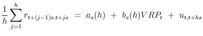
In parallel to the general multi-period return regression defined in equation (1), our monthly return regressions for each of the individual countries may be expressed as,
| (2) |
where
The actual estimates for ![]() and the corresponding
and the corresponding ![]() -statistics
obviously differ somewhat across the countries. However, with the exception of France and the U.S., the estimated coefficients all show the same general pattern starting out fairly low and insignificant at the shortest one-month horizon, rising to their largest values at 3-5 months, and then
gradually declining thereafter for longer return horizons. These similarities are also evident in Figure 6, which displays the regression coefficients for the variance risk
premia along with the conventional 95-percent confidence bands based on two NW standard errors.19
-statistics
obviously differ somewhat across the countries. However, with the exception of France and the U.S., the estimated coefficients all show the same general pattern starting out fairly low and insignificant at the shortest one-month horizon, rising to their largest values at 3-5 months, and then
gradually declining thereafter for longer return horizons. These similarities are also evident in Figure 6, which displays the regression coefficients for the variance risk
premia along with the conventional 95-percent confidence bands based on two NW standard errors.19
These general patterns in the estimated values of ![]() naturally translate into very similar patterns in the corresponding regression
naturally translate into very similar patterns in the corresponding regression ![]() 's. In particular, looking at the plots in Figure 7, all of the
's. In particular, looking at the plots in Figure 7, all of the ![]() 's exhibit an almost identical hump-shaped pattern with the degree of predictability maximized at the 4 months horizon. Of course, the actual values of the
's exhibit an almost identical hump-shaped pattern with the degree of predictability maximized at the 4 months horizon. Of course, the actual values of the ![]() 's again vary somewhat across the different indices, achieving a maximum of only 0.96 percent for the Nikkei 225 compared to 14.18 percent for the S&P 500.20
's again vary somewhat across the different indices, achieving a maximum of only 0.96 percent for the Nikkei 225 compared to 14.18 percent for the S&P 500.20
Taken as whole, the results in Table 4 and the significance of the country specific VRP's as predictor variables help to underscore the significance of the existing results based exclusively on the U.S. data. The similarities in the patterns obtained across countries also suggest that even stronger results may be available by pooling the regressions and entertaining the notion of a common "global" variance risk premium. We explore these ideas next.
3.3 Global Variance Risk Premium and Panel Regressions
Our definition of a "global" variance risk premium is based on a simple capitalization weighted average of the country specific variance risk premia,
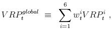 |
where
The results for the regressions obtained by replacing the country specific ![]() 's in equation (2) with the new
's in equation (2) with the new
![]() index,
index,
are reported in Table 5, along with the corresponding
These striking cross country similarities are also immediately evident from the plots of the estimated regression coefficients and the two NW-based standard error bands in Figure 9. Not only do the individual country estimates for the ![]() 's look very similar, the confidence bands also become much tighter compared
to the country specific regressions discussed above. Further along these lines, Figure 10 shows the general patterns in the predictability, as measured by the
's look very similar, the confidence bands also become much tighter compared
to the country specific regressions discussed above. Further along these lines, Figure 10 shows the general patterns in the predictability, as measured by the ![]() 's, to be very similarly shaped for the different countries, with uniform peaks at the 4 months return horizon.22
's, to be very similarly shaped for the different countries, with uniform peaks at the 4 months return horizon.22
Going one step further, we next restrict the coefficients for the "global" variance risk premium to be the same across countries,
as a way to further enhance the efficiency of the estimates. The corresponding panel regression estimates for the
These key empirical findings are succinctly summarized in Figure 11, which plots the panel regression estimates for ![]() based on the country specific and "global" VRP measures along with two NW standard error bands (top two panels), and the corresponding panel regression
based on the country specific and "global" VRP measures along with two NW standard error bands (top two panels), and the corresponding panel regression ![]() 's (bottom two panels). The
's (bottom two panels). The
![]() -based regressions (depicted in the right two panels) obviously result in sharper coefficient estimates and stronger average predictability across the six countries, compared to
the individual country
-based regressions (depicted in the right two panels) obviously result in sharper coefficient estimates and stronger average predictability across the six countries, compared to
the individual country ![]() regression (depicted in the left two panels).
regression (depicted in the left two panels).
The panel regression ![]() 's, of course, mask important cross-country differences in the degree of predictability. We therefore also show in Figure 12 the country specific implied
's, of course, mask important cross-country differences in the degree of predictability. We therefore also show in Figure 12 the country specific implied ![]() 's obtained by evaluating the
regressions in equation (3) at the more precisely estimated common
's obtained by evaluating the
regressions in equation (3) at the more precisely estimated common
![]() and
and
![]() obtain from the panel regressions in equation (4).
Interestingly, comparing Figure 12 to the earlier Figure 10 for the individual country regressions, it is clear that the added precision afforded by restricting the
obtain from the panel regressions in equation (4).
Interestingly, comparing Figure 12 to the earlier Figure 10 for the individual country regressions, it is clear that the added precision afforded by restricting the ![]() and
and ![]() coefficients to be the same across countries sacrifices very little in terms of the implied predictability.
coefficients to be the same across countries sacrifices very little in terms of the implied predictability.
To assess the robustness of these impressive empirical findings, the next panel in Table 6 reports the results obtained by including a capitalization weighted average of the
country specific P/E ratios as an additional regressor. Consistent with the results for the U.S. market in isolation reported in BTZ2009, the "global" P/E ratio adds nothing to the predictability afforded by
![]() within the one-year horizons reported in the table, leaving all of the estimates for
within the one-year horizons reported in the table, leaving all of the estimates for ![]() and the
and the ![]() 's the same to within the second decimal place. The predictability of the "global" variance risk premium is effectively orthogonal to that documented in
the existing literature based on more traditional macro-finance variables, such as the P/E ratio, dividend yields, and consumption-wealth ratios, which are typically only significant over longer multi-year return horizons (see, e.g., the classic studies by Fama and French, 1988, Campbell and Shiller, 1988b; Lettau and Ludvigson, 2001).24
's the same to within the second decimal place. The predictability of the "global" variance risk premium is effectively orthogonal to that documented in
the existing literature based on more traditional macro-finance variables, such as the P/E ratio, dividend yields, and consumption-wealth ratios, which are typically only significant over longer multi-year return horizons (see, e.g., the classic studies by Fama and French, 1988, Campbell and Shiller, 1988b; Lettau and Ludvigson, 2001).24
To further highlight the predictive gains afforded by the use of our "global" VRP as opposed to the own country VRP's, the last two panels in Table 6 report the results obtained by including each individual country's premium in a panel regression,
| (5) |
While the results still point to overall efficiency gains from the panel regression setting relative to the individual country specific regressions in Table 4, the magnitude of the return predictability is obviously much lower than for
To help better understand the economic mechanisms underlying these new empirical findings, we next present a stylized two-country equilibrium model. This relatively simple model provides a possible rationale for why the estimated "global" VRP regression coefficients are fairly similar across
countries, and why the ![]() 's for the panel regressions depicted in Figure 11 are generally larger for the "global" VRP than for the "local" VRP's, except for the U.S.
's for the panel regressions depicted in Figure 11 are generally larger for the "global" VRP than for the "local" VRP's, except for the U.S.
3.4 Global Variance Risk in Equilibrium
Our two-country model is based on a direct extension of the "long-run risk" model in BTZ2009.25 Specifically, denoting the geometric growth rate of
consumption in country ![]() by
by
![]() , we will assume that
, we will assume that
| (6) | ||
| (7) | ||
| (8) |
where
| (9) |
This trivially implies time-varying conditional correlations, unless the parameters are identical across the covariance and two variance processes.27
We assume that the two international equity markets are fully integrated. We further assume the existence of a global representative agent with a claim on the world aggregate consumption, defined as the per capita weighted average consumption in each of the two countries, say
![]() . Moreover, this agent is endowed with Epstein-Zin-Weil recursive preferences of the form
. Moreover, this agent is endowed with Epstein-Zin-Weil recursive preferences of the form
| (10) |
In the specific calibration reported on below, we follow Bansal and Yaron (2004) and BTZ2009 in fixing the discount rate at
The parameters for the consumption dynamics are calibrated to mimic the U.S. as country "1", and the U.K. as country "2". In particular, following BTZ2009 we fix the base parameters for the U.S. at ![]() =0.0015,
=0.0015,
![]() =0.979,
=0.979,
![]() =
=
![]() ),
), ![]() =0.80,
=0.80, ![]() =1.0*10e-6, and
=1.0*10e-6, and ![]() =0.001, respectively. For simplicity, we treat the weights used in the calculation of
"global" consumption as constant and equal to
=0.001, respectively. For simplicity, we treat the weights used in the calculation of
"global" consumption as constant and equal to
![]() =0.855 and
=0.855 and
![]() =0.145, corresponding to the consumption shares at the end of the sample.
=0.145, corresponding to the consumption shares at the end of the sample.
The relevance of allowing for time-varying cross-country covariances is highlighted by Figure 13, which plots exponentially weighted moving average estimates of U.S. variances, and
U.S.-U.K. covariances and correlations from 1951 to 2009.28 Although the U.S.-U.K. consumption covariances clearly changes through time, the process is not
as persistent as the process for the U.S. variance depicted in the top panel. We consequently set ![]() =0.85 and
=0.85 and
![]() . Finally, we set the parameter
. Finally, we set the parameter
![]() =
=
![]() to reflect the generally higher variability of UK consumption growth.
to reflect the generally higher variability of UK consumption growth.
Turning to the actual calibration results, the top two panels in Figure 14 show the implied regression coefficients for the "local" (dashed lines) and "global" (solid lines) VRP
regressions for each of the two countries, while the bottom two panels show the implied ![]() 's from the "local" (dashed lines) and "global" (solid lines) VRP panel regressions.29 The model-implied regressions in the figure generally match the qualitative features in the actual international return regressions quite well.
's from the "local" (dashed lines) and "global" (solid lines) VRP panel regressions.29 The model-implied regressions in the figure generally match the qualitative features in the actual international return regressions quite well.
First, the implied slope coefficients for
![]() in the two individual country regressions tend to be close across all horizons. For instance, at the four-month horizon, the model implied slope coefficients equal 0.34 and 0.33
for the U.S. and U.K., respectively, both of which are well within two standard errors of their corresponding estimates reported in Table 5. Of course, these numbers are also
very close to the estimate of 0.32 for the six-country panel regression in Table 6.
in the two individual country regressions tend to be close across all horizons. For instance, at the four-month horizon, the model implied slope coefficients equal 0.34 and 0.33
for the U.S. and U.K., respectively, both of which are well within two standard errors of their corresponding estimates reported in Table 5. Of course, these numbers are also
very close to the estimate of 0.32 for the six-country panel regression in Table 6.
Second, the exposure to the "local" VRP is systematically lower than the exposure to the "global" VRP for the smaller country in the model (U.K.), directly mirroring the empirical results. Conversely, for the larger country (U.S.), the "local" VRP gives rise to marginally higher slope coefficients than the "global" VRP within the model, again directly mirroring the actual empirical results. Specifically, focusing again on the four-month horizon, the slope coefficient implied by the model equals 0.17 for the U.K. compared to 0.15 for the actual U.K. regression. In comparison, the model implied slope coefficient for the U.S. equals 0.40, compared to 0.36 for the actual "local" U.S. regression.
Third, looking at the ![]() 's from the corresponding panel regressions in the bottom two panels of Figure 14, both of the plots exhibit a hump shaped pattern with an apparent peak at the 2-4 month horizons. This overall shape closely matches that for the actual six-country panel regressions depicted in the bottom two panels in Figure 11. Of course, the values of the
's from the corresponding panel regressions in the bottom two panels of Figure 14, both of the plots exhibit a hump shaped pattern with an apparent peak at the 2-4 month horizons. This overall shape closely matches that for the actual six-country panel regressions depicted in the bottom two panels in Figure 11. Of course, the values of the ![]() 's from the theoretical model are somewhat
muted compared to the six-country panel regressions
's from the theoretical model are somewhat
muted compared to the six-country panel regressions ![]() 's. Importantly, however, the model implied panel regression
's. Importantly, however, the model implied panel regression ![]() 's based on
's based on
![]() uniformly dominate the "local" VRP panel regression
uniformly dominate the "local" VRP panel regression ![]() 's. Again,
these theoretical implications directly mirror the empirical results for the six-country panel regressions in Figure 11. Intuitively, the "global" VRP effectively isolates the
aggregate world-wide economic uncertainty that is being priced in both markets, in turn providing better overall predictions for the future returns than the "local" VRP's.30
's. Again,
these theoretical implications directly mirror the empirical results for the six-country panel regressions in Figure 11. Intuitively, the "global" VRP effectively isolates the
aggregate world-wide economic uncertainty that is being priced in both markets, in turn providing better overall predictions for the future returns than the "local" VRP's.30
In a sum, while the qualitative implications form our stylized equilibrium model are generally in line with the international predictability patterns documented in the data, some of the quantitative implications from the model fall short in explaining the magnitude of the effects. However, we purposely kept the model relatively simple, involving only two independent volatility shocks. It is certainly possible that by extending the basic model setup to include additional sources of covariance, or correlation, risks, a full-fledged risk-based explanation for the new international evidence may be feasible.
4 Conclusion
A number of recent studies have argued that the aggregate U.S. stock market return is predictable over relatively short 2-4 month horizons by the difference between options implied and actual realized variances, or the so-called variance risk premium. We provide extensive Monte Carlo simulation evidence that this newly documented predictability is not due to finite sample biases in the statistical inference procedures, and that the hump-shape in the degree of predictability with a maximum at the 2-4 month horizons is entirely consistent with the implications from an empirically realistic bivariate daily time series model for the returns and variance risk premia.
Further corroborating the existing empirical evidence for the U.S. market, we show that the same basic predictive relationship between future returns and current variance risk premia holds true for a set of five other countries, although the magnitude of the predictability and the statistical
significance of the own country variance risk premia tend to be somewhat muted relative to those for the U.S. Meanwhile, regressing the individual country returns on a capitalization weighted "global" variance risk premium, results in almost identical shapes in the degree of predictability across
horizons and uniformly larger ![]() -statistics for all of the countries in the sample. Further restricting the regression coefficients and the compensation for the "global" variance risk to be
the same across countries, we find even stronger results and highly significant test statistics, with the degree of predictability maximized at the four month horizon. By contrast, the predictability documented in the existing literature based on more traditional macro-finance variables are
generally only significant over longer multi-year return horizons.
-statistics for all of the countries in the sample. Further restricting the regression coefficients and the compensation for the "global" variance risk to be
the same across countries, we find even stronger results and highly significant test statistics, with the degree of predictability maximized at the four month horizon. By contrast, the predictability documented in the existing literature based on more traditional macro-finance variables are
generally only significant over longer multi-year return horizons.
These new empirical findings naturally raise the question of why the "global" variance risk premium works so well as a predictor variable, and why the predictability is restricted to within-year horizons. Building on the equilibrium based model in Bollerslev, Tauchen, and Zhou (2009), we argue that the "global" variance risk premium may be seen as a proxy for world-wide aggregate economic uncertainty. We also show why this "global" variance risk premium may serve as a more effective predictor variable for future international equity returns than the own country's individual variance risk premium.
Alternatively, following the analysis in Bekaert, Engstrom, and Xing (2009), the variance risk premium may be interpreted as a measure of aggregate risk aversion in world financial markets, or a summary measure of disagreements in beliefs across international market participants, as discussed in Buraschi, Trojani, and Vedolin (2010). All of these competing explanations are likely at work to some degree, and we leave it for future research to more clearly sort out the extent to which each of these competing explanations best accounts for the strong international return predictability embodied in the "global" variance risk premium documented here.
A. Two-Country Equilibrium Model Solution
Following Epstein and Zin (1989), the logarithm of the world unique intertemporal marginal rate of substitution, ![]() =
=
![]() , must satisfy,
, must satisfy,
| (A.1) |
where
| (A.2) |
| (A.3) |
where
Combining the equations for
![\displaystyle r^{i}_{t+1} = c_{i,r}+\sum_{l=1}^2 A_{r_{i},g_{l}}\sigma^{2}_{g_{l},t}+A_{r_{i},q}q_{t}+ A_{r_{i},cv,ij}cv_{t,ij}+\sqrt{q_{t}}k_{i,1}[A_{i,\varphi}z_{\sigma,t+1}+A_{i,q}\varphi_{q}z_{q,t+1}] \\ +\sigma_{g_{i},t}z_{g_{i},t+1},](img180.gif) |
(A.6) |
where
Next, utilizing the standard no-arbitrage condition
![]() , the parameters for the "world" in equation (A.4) may be solved as,34
, the parameters for the "world" in equation (A.4) may be solved as,34
![\displaystyle =\frac{\log(\delta)+(1-\varphi^{-1})\mu_{g}+k_{0}+k_{1}[\sum A_{\sigma_{j}}\alpha_{\sigma}\varphi_{q,j}+A_{q}\alpha_{q}+A_{cv,ij}\alpha_{cv}]}{1-k_{1}},](img193.gif) |
||
 |
||
 |
||
Similarly, the parameters for the individual countries in equation (A.5) may be solved as,35
![\displaystyle =\frac{\log(\delta)+ (1-\varphi^{-1})\mu_{g}+k_{i,0}+k_{i,1}[\sum A_{i,\sigma_{j}}\alpha_{\sigma}\varphi_{q,j}+A_{i,q}\alpha_{q}+ A_{i,cv,ij}\alpha_{cv,ij}]}{1-k_{i,1}},](img202.gif) |
||
 |
||
 |
||
 |
||
 |
||
 |
||
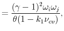
Going one step further and building on the derivations in BTZ2009, the two country specific VRP's may be approximated as,
| (A.7) |
where
Based on these expressions, it is now possible to derive the slope coefficients from regressing country ![]() 's return on country
's return on country ![]() 's VRP,
's VRP,
 |
(A.8) |
as well as the slope coefficient from regressing country
 |
(A.9) |
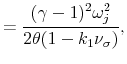
The final expressions for the "global" and "local" panel regressions discussed in the main text may be derived analogously. In particular, it is possible to show that
 |
(A.10) |
and
 |
(A.11) |
where
 |
 |
 |
||
![\displaystyle +2\sum^2_{l=1}A_{r_{i},g_{l}}A_{r_{i},cv,ij}Cov(\sigma^{2}_{g_{l},t},cv_{t,ij})+k^{2}_{i,1}[(A^{2}_{i,\varphi}+A^{2}_{i,q}\varphi^{2}_{q})E(q_{t})]+E(\sigma^2_{g_{i},t}),](img228.gif) |
 |
||
 |
 |
and the model-implied moments entering the above expressions are given by,
 |
 |
 |
Bibliography
"Stock Return Predictability: Is it There?" Review of Financial Studies, vol. 20, 651-707. "Predicting Returns with Managerial Decision Variables: Is There a Small-Sample Bias?" Journal of Finance, vol. 61, 1711-1730. "The Baltic Dry Index as a Predictor of Global Stock Returns, Commodity Returns, and Global Economic Activity," Working Paper, Smith School of Business, University of Maryland. "A Long-Run Risks Explanation of Predictability Puzzles in Bond and Currency Markets," Working Paper, Fuqua School of Business, Duke University, and The Wharton School, University of Pennsylvania. "Risks for the Long Run: A Potential Resolution of Asset Pricing Puzzles," The Journal of Finance, vol. 59, 1481-1509. "Risk, Uncertainty and Asset Prices," Journal of Financial Economics, vol. 91, 59-82. "Characterizing Predictable Components in Excess Returns on Equity and Foreign Exchange Markets," Journal of Finance, vol. 47, 467-509. "Volatility in Equilibrium: Asymmetries and Dynamics Dependencies," Review of Finance, forthcoming. "Expected Stock Returns and Variance Risk Premia," Review of Financial Studies, vol. 22, 4463-4492. "Quasi-Maximum Likelihood Estimation and Inference in Dynamic Models with Time-Varying Covariances," Econometric Reviews, vol. 11, 143-172. "The Myth of Long-Horizon Predictability," Review of Financial Studies, vol. 21, 1577-1605. "Economic Uncertainty, Disagreement, and Credit Markets," Working Paper, London School of Economics. "Robust Inference with Multiway Clustering," Journal of Business and Economic Statistics, vol. 29, 238-249. "Why Long Horizons? A Study of Power Against Persistent Alternatives," Journal of Empirical Finance, vol. 8, 459-491. "Predicting Stock Returns in the United States and Japan: A Study of Long-Term Capital Market Integration," Journal of Finance, vol. 47, 63-49. The Econometrics of Financial Markets, Princeton University Press, Princeton, NJ. "The Dividend-Price Ratio and Expectations of Future Dividends and Discount Factors," Review of Financial Studies, vol. 1, 195-228. "Stock Prices, Earnings, and Expected Dividends," Journal of Finance, vol. 43, 661-676. "Efficient Tests of Stock Return Predictability," Journal of Financial Economics, vol. 81, 27-60. "What's Vol Got to Do With It," Review of Financial Studies, vol. 24, 1-45. "Dynamic Conditional Correlation: A Simple Class of Multivariate GARCH Models," Journal of Business and Economic Statistics, vol. 20, 339-350. "Substitution, Risk Aversion and the Intertemporal Behavior of Consumption and Asset Returns: A Theoretical Framework," Econometrica, vol. 57, 937-969. "Dividend Yields and Expected Stock Returns," Journal of Financial Economics, vol. 22, 3-25. "The Risk and Predictability of International Equity Returns," Review of Financial Studies, vol. 6, 527-566. "Spurious Regressions in Financial Economics?" Journal of Finance, vol. 58, 1393-1414. "Variable Rare Disasters: An Exactly Solved Framework for Ten Puzzles in Macro-Finance," Working Paper, Stern School of Business, New York University. "A Comprehensive Look at the Empirical Performance of Equity Premium Prediction," Review of Financial Studies, vol. 21, 1455-1508. "The World Price of Covariance Risk," Journal of Finance, vol. 46, 111-157. "Predicting Global Stock Returns," Journal of Financial and Quantitative Analysis, vol. 45, 49-80. "Dividend Yields and Expected Stock Returns: Alternative Procedures for Inference and Measurement," Review of Financial Studies, vol. 5, 357-386. "Tail Risk and Asset Prices," Working Paper, Booth School of Business, University of Chicago. "Consumption, Aggregate Wealth, and Expected Stock Returns," Journal of Finance, vol. 56, 815-849. "The Variance Risk Premium Around the World," Working Paper, Department of Finance, Tilburg University, The Netherlands. "Short-Run Bond Risk Premia," Working Paper, London School of Economics, and Federal Reserve Board, Washington D.C. "A Simple Positive Semi-Definite, Heteroskedasticity and Autocorrelation Consistent Covariance Matrix," Econometrica, vol. 55, 703-708. "Stock Market Volatility and the Forecasting Accuracy of Implied Volatility Indices," Working Paper, Graduate School of Economics and School of International Public Policy, Osaka University, Japan. "Estimating Standard Errors in Finance Panel Data Sets: Comparing Approaches," Review of Financial Studies, vol. 22, 435-480. "International Stock Return Predictability: What is the Role of United States?" Working Paper, Olin School of Business, Washington University in St. Louis. "Implied Volatility Indices - A Review," Working Paper, Department of Business Administration, University of Patras, Greece. "Predictive Regressions," Journal of Financial Economics, vol. 54, 375-421. "A Long-Run Risks Model with Long- and Short-Run Volatilities: Explaining Predictability and Volatility Risk Premium," Working Paper, Olin School of Business, Washington University. "Variance Risk Premia, Asset Predictability Puzzles, and Macroeconomic Uncertainty," Working Paper, Federal Reserve Board, Washington D.C.The table reports the simulated 95-percentiles in the finite sample distributions of
|
|
|
|
|||||||||
| 20 | 2.445 | 2.182 | 3.036 | 4 | 2.434 | 2.212 | 2.971 | 1 | 2.260 | 2.276 | 3.017 |
| 40 | 2.602 | 2.112 | 4.804 | 8 | 2.600 | 2.078 | 4.800 | 2 | 2.520 | 2.187 | 4.837 |
| 60 | 2.815 | 2.085 | 5.756 | 12 | 2.805 | 2.016 | 5.790 | 3 | 2.788 | 2.083 | 5.774 |
| 80 | 2.969 | 2.107 | 6.324 | 16 | 2.967 | 2.031 | 6.345 | 4 | 2.941 | 2.106 | 6.315 |
| 120 | 3.054 | 2.152 | 7.639 | 24 | 3.095 | 2.098 | 7.615 | 6 | 3.220 | 2.124 | 7.502 |
| 180 | 3.289 | 2.171 | 8.594 | 36 | 3.322 | 2.113 | 8.482 | 9 | 3.314 | 2.163 | 8.192 |
| 240 | 3.400 | 2.229 | 8.951 | 48 | 3.476 | 2.146 | 8.682 | 12 | 3.509 | 2.186 | 8.679 |
The table reports the simulated power of the size-adjusted 5-percent
| 20 | 0.919 | 0.873 | 4 | 0.910 | 0.852 | 1 | 0.886 | 0.807 |
| 40 | 0.888 | 0.808 | 8 | 0.877 | 0.799 | 2 | 0.845 | 0.762 |
| 60 | 0.804 | 0.725 | 12 | 0.793 | 0.729 | 3 | 0.768 | 0.711 |
| 80 | 0.710 | 0.630 | 16 | 0.709 | 0.639 | 4 | 0.686 | 0.627 |
| 120 | 0.567 | 0.474 | 24 | 0.553 | 0.481 | 6 | 0.507 | 0.497 |
| 180 | 0.375 | 0.352 | 36 | 0.371 | 0.352 | 9 | 0.368 | 0.350 |
| 240 | 0.288 | 0.283 | 48 | 0.285 | 0.289 | 12 | 0.277 | 0.302 |
The monthly excess returns are in annualized percentage form. The variance risk premia are in monthly percentage-squared form. The "global" index of variance risk premium are defined in the main text. The sample period extends from January 2000 to December 2010.
|
|
VRP |
|
VRP |
|
VRP |
|
VRP |
|
VRP |
|
VRP |
VRP |
|
| Mean | -6.52 | 4.13 | -2.76 | 6.01 | -4.82 | 8.16 | -6.12 | 13.26 | -2.15 | 5.36 | -3.70 | 7.69 | 8.15 |
| Std. Dev | 67.72 | 41.45 | 82.53 | 32.74 | 52.87 | 32.63 | 73.08 | 35.26 | 52.04 | 29.03 | 57.82 | 34.08 | 32.14 |
| Skewness | -0.62 | -4.97 | -0.85 | -2.90 | -0.68 | -5.35 | -0.79 | -5.23 | -0.70 | -4.21 | -0.67 | -5.06 | -5.62 |
| Kurtosis | 3.74 | 43.09 | 5.45 | 16.67 | 3.56 | 47.38 | 4.67 | 52.11 | 3.57 | 31.83 | 3.93 | 39.41 | 49.01 |
| AR(1) | 0.11 | 0.27 | 0.08 | 0.07 | 0.07 | 0.34 | 0.15 | 0.18 | 0.27 | 0.12 | 0.16 | 0.50 | 0.46 |
| CAC 40 | DAX | FTSE 100 | Nikkei 225 | SMI | S&P 500 | |
| CAC 40 | 1.00 | 0.94 | 0.89 | 0.59 | 0.84 | 0.85 |
| DAX | 1.00 | 0.83 | 0.56 | 0.81 | 0.82 | |
| FTSE 100 | 1.00 | 0.62 | 0.80 | 0.87 | ||
| Nikkei 225 | 1.00 | 0.56 | 0.64 | |||
| SMI | 1.00 | 0.77 | ||||
| S&P 500 | 1.00 |
| CAC 40 | DAX | FTSE 100 | Nikkei 225 | SMI | S&P 500 | Global | |
| CAC 40 | 1.00 | 0.83 | 0.89 | 0.72 | 0.83 | 0.85 | 0.90 |
| DAX | 1.00 | 0.78 | 0.59 | 0.88 | 0.71 | 0.77 | |
| FTSE 100 | 1.00 | 0.78 | 0.86 | 0.90 | 0.94 | ||
| Nikkei 225 | 1.00 | 0.69 | 0.72 | 0.81 | |||
| SMI | 1.00 | 0.74 | 0.81 | ||||
| S&P 500 | 1.00 | 0.99 | |||||
| Global | 1.00 |
The results are based on the monthly regression in equation (2).
| Index / Monthly Horizon | 1 | 2 | 3 | 4 | 5 | 6 | 9 | 12 |
| CAC 40 Constant | -7.41 | -8.07 | -8.13 | -8.30 | -8.35 | -8.30 | -8.52 | -8.39 |
| CAC 40 Constant |
(-1.04) | (-1.16) | (-1.18) | (-1.20) | (-1.19) | (-1.18) | (-1.14) | (-1.10) |
| CAC 40 VRP |
0.22 | 0.22 | 0.22 | 0.21 | 0.16 | 0.11 | 0.06 | 0.04 |
| CAC 40 VRP |
(2.71) | (3.59) | (3.30) | (3.79) | (3.86) | (3.01) | (1.37) | (0.88) |
| CAC 40 Adj. R |
0.99 | 2.61 | 3.89 | 4.88 | 3.19 | 1.36 | -0.03 | -0.32 |
| DAX 30 Constant | -2.72 | -4.58 | -4.78 | -5.28 | -5.29 | -4.76 | -4.63 | -4.80 |
| DAX 30 Constant |
(-0.30) | (-0.54) | (-0.58) | (-0.66) | (-0.66) | (-0.58) | (-0.54) | (-0.56) |
| DAX 30 VRP |
-0.01 | 0.19 | 0.19 | 0.24 | 0.22 | 0.13 | 0.07 | 0.10 |
| DAX 30 VRP |
(-0.06) | (1.10) | (1.51) | (2.04) | (2.58) | (1.55) | (1.44) | (2.25) |
| DAX 30 Adj. R |
-0.77 | 0.34 | 0.76 | 2.40 | 2.42 | 0.39 | -0.30 | 0.52 |
| FTSE 100 Constant | -4.67 | -5.50 | -6.28 | -6.56 | -6.51 | -6.38 | -6.08 | -5.86 |
| FTSE 100 Constant |
(-0.82) | (-0.99) | (-1.19) | (-1.25) | (-1.23) | (-1.20) | (-1.12) | (-1.09) |
| FTSE 100 VRP |
-0.02 | 0.05 | 0.13 | 0.15 | 0.13 | 0.10 | 0.02 | -0.01 |
| FTSE 100 VRP |
(-0.20) | (0.91) | (3.02) | (3.86) | (4.14) | (2.22) | (0.59) | (-0.29) |
| FTSE 100 Adj. R |
-0.76 | -0.61 | 0.93 | 2.55 | 1.84 | 0.94 | -0.72 | -0.82 |
| Nikkei 225 Constant | -6.00 | -6.75 | -8.63 | -8.79 | -7.97 | -7.57 | -6.10 | -5.67 |
| Nikkei 225 Constant |
(-0.80) | (-0.90) | (-1.15) | (-1.20) | (-1.10) | (-1.04) | (-0.79) | (-0.73) |
| Nikkei 225 VRP |
-0.01 | 0.03 | 0.14 | 0.16 | 0.10 | 0.08 | 0.00 | 0.01 |
| Nikkei 225 VRP |
(-0.09) | (0.27) | (1.46) | (1.80) | (1.22) | (0.91) | (0.04) | (0.36) |
| Nikkei 225 Adj. R |
-0.77 | -0.75 | 0.29 | 0.95 | 0.11 | -0.19 | -0.83 | -0.81 |
| SMI Constant | -2.39 | -3.07 | -3.24 | -3.81 | -3.91 | -3.87 | -3.77 | -3.76 |
| SMI Constant |
(-0.36) | (-0.47) | (-0.51) | (-0.62) | (-0.64) | (-0.63) | (-0.59) | (-0.57) |
| SMI VRP |
0.04 | 0.15 | 0.15 | 0.24 | 0.22 | 0.18 | 0.10 | 0.09 |
| SMI VRP |
(0.37) | (1.76) | (1.49) | (2.37) | (3.24) | (2.88) | (2.43) | (3.42) |
| SMI Adj. R |
-0.71 | 0.40 | 0.73 | 3.55 | 3.53 | 2.59 | 0.71 | 0.78 |
| S&P 500 Constant | -6.93 | -6.88 | -7.16 | -7.09 | -6.65 | -6.08 | -5.31 | -5.02 |
| S&P 500 Constant |
(-1.30) | (-1.29) | (-1.38) | (-1.34) | (-1.23) | (-1.11) | (-0.95) | (-0.94) |
| S&P 500 VRP |
0.42 | 0.40 | 0.39 | 0.36 | 0.28 | 0.18 | 0.04 | 0.00 |
| S&P 500 VRP |
(5.11) | (5.29) | (8.43) | (8.80) | (6.52) | (3.83) | (0.90) | (0.13) |
| S&P 500 Adj. R |
5.40 | 8.72 | 13.13 | 14.18 | 9.40 | 4.06 | -0.54 | -0.84 |
The results are based on the monthly regression in equation (3).
| Index / Monthly Horizon | 1 | 2 | 3 | 4 | 5 | 6 | 9 | 12 |
| CAC 40 Constant | -8.51 | -10.00 | -9.96 | -10.09 | -9.79 | -9.16 | -8.58 | -8.28 |
| CAC 40 Constant |
(-1.15) | (-1.39) | (-1.43) | (-1.44) | (-1.39) | (-1.29) | (-1.15) | (-1.09) |
| CAC 40 VRP
|
0.24 | 0.35 | 0.33 | 0.33 | 0.26 | 0.16 | 0.04 | 0.01 |
| CAC 40 VRP
|
(2.44) | (4.52) | (6.21) | (8.21) | (6.95) | (3.58) | (0.96) | (0.22) |
| CAC 40 Adj. R |
0.58 | 4.22 | 5.99 | 7.43 | 5.27 | 1.87 | -0.59 | -0.83 |
| DAX 30 Constant | -4.72 | -6.44 | -6.66 | -6.96 | -6.55 | -5.55 | -4.56 | -4.39 |
| DAX 30 Constant |
(-0.54) | (-0.75) | (-0.81) | (-0.85) | (-0.79) | (-0.67) | (-0.53) | (-0.51) |
| DAX 30 VRP
|
0.24 | 0.37 | 0.38 | 0.39 | 0.33 | 0.20 | 0.05 | 0.02 |
| DAX 30 VRP
|
(2.43) | (2.61) | (6.26) | (7.90) | (4.07) | (2.32) | (0.72) | (0.31) |
| DAX 30 Adj. R |
0.10 | 3.20 | 5.10 | 7.21 | 5.85 | 1.91 | -0.63 | -0.82 |
| FTSE 100 Constant | -5.87 | -6.52 | -7.00 | -7.03 | -6.89 | -6.58 | -6.08 | -5.83 |
| FTSE 100 Constant |
(-1.09) | (-1.23) | (-1.38) | (-1.38) | (-1.33) | (-1.26) | (-1.13) | (-1.09) |
| FTSE 100 VRP
|
0.13 | 0.18 | 0.22 | 0.22 | 0.18 | 0.13 | 0.02 | -0.01 |
| FTSE 100 VRP
|
(1.78) | (1.85) | (3.44) | (5.07) | (3.79) | (2.21) | (0.56) | (-0.38) |
| FTSE 100 Adj. R |
-0.16 | 1.40 | 4.23 | 5.55 | 4.30 | 2.02 | -0.70 | -0.78 |
| Nikkei 225 Constant | -7.31 | -7.70 | -8.72 | -8.66 | -8.08 | -7.49 | -6.00 | -5.45 |
| Nikkei 225 Constant |
(-0.94) | (-1.03) | (-1.19) | (-1.20) | (-1.12) | (-1.04) | (-0.79) | (-0.71) |
| Nikkei 225 VRP
|
0.15 | 0.16 | 0.24 | 0.25 | 0.19 | 0.12 | -0.01 | -0.01 |
| Nikkei 225 VRP
|
(1.13) | (2.51) | (4.44) | (5.05) | (3.15) | (1.67) | (-0.17) | (-0.19) |
| Nikkei 225 Adj. R |
-0.36 | 0.11 | 1.97 | 2.81 | 1.77 | 0.47 | -0.81 | -0.84 |
| SMI Constant | -3.58 | -4.53 | -4.76 | -5.08 | -4.89 | -4.50 | -3.65 | -3.45 |
| SMI Constant |
(-0.55) | (-0.71) | (-0.77) | (-0.82) | (-0.79) | (-0.73) | (-0.57) | (-0.53) |
| SMI VRP
|
0.17 | 0.28 | 0.29 | 0.32 | 0.27 | 0.20 | 0.05 | 0.02 |
| SMI VRP
|
(1.51) | (5.78) | (5.32) | (7.70) | (8.39) | (5.62) | (1.52) | (0.59) |
| SMI Adj. R |
0.40 | 4.10 | 6.10 | 8.92 | 7.54 | 4.47 | -0.34 | -0.76 |
| S&P 500 Constant | -7.03 | -6.95 | -7.41 | -7.40 | -6.88 | -6.29 | -5.49 | -5.20 |
| S&P 500 Constant |
(-1.32) | (-1.32) | (-1.46) | (-1.43) | (-1.30) | (-1.17) | (-1.00) | (-0.98) |
| S&P 500 VRP
|
0.41 | 0.38 | 0.40 | 0.38 | 0.29 | 0.20 | 0.06 | 0.03 |
| S&P 500 VRP
|
(4.98) | (5.01) | (6.93) | (7.88) | (5.70) | (3.40) | (1.24) | (0.68) |
| S&P 500 Adj. R |
4.43 | 7.05 | 12.04 | 13.69 | 9.04 | 4.31 | -0.16 | -0.62 |
The results are based on on the monthly "global" and county-specific panel regressions in equations (4) and (5), respectively. NW-based
| "Global" Regressors Horizon (mos) | 1 | 2 | 3 | 4 | 5 | 6 | 9 | 12 |
| Constant | -6.17 | -7.02 | -7.42 | -7.54 | -7.18 | -6.60 | -5.73 | -5.44 |
| Constant |
(-2.15) | (-2.51) | (-2.74) | (-2.78) | (-2.64) | (-2.42) | (-2.12) | (-2.07) |
| VRP
|
0.22 | 0.29 | 0.31 | 0.31 | 0.25 | 0.17 | 0.04 | 0.01 |
| VRP
|
(4.66) | (6.60) | (9.70) | (11.21) | (9.43) | (6.04) | (1.41) | (0.41) |
| Adj. R |
1.08 | 3.43 | 5.85 | 7.46 | 5.72 | 2.81 | 0.04 | -0.12 |
| Constant | -14.90 | -10.73 | -2.25 | 4.05 | 4.41 | 2.03 | -8.12 | -13.83 |
| Constant |
(-0.63) | (-0.47) | (-0.11) | (0.20) | (0.23) | (0.11) | (-0.46) | (-0.83) |
| VRP
|
0.22 | 0.28 | 0.32 | 0.32 | 0.26 | 0.18 | 0.03 | 0.00 |
| VRP
|
(4.45) | (5.34) | (9.34) | (10.81) | (8.17) | (5.28) | (1.18) | (0.03) |
| log( |
2.70 | 1.14 | -1.60 | -3.57 | -3.57 | -2.66 | 0.73 | 2.59 |
| log( |
(0.37) | (0.16) | (-0.25) | (-0.59) | (-0.62) | (-0.47) | (0.14) | (0.53) |
| Adj. R |
0.99 | 3.32 | 5.75 | 7.51 | 5.80 | 2.81 | -0.08 | -0.06 |
| Country-Specific Regressors Horizon (mos) | 1 | 2 | 3 | 4 | 5 | 6 | 9 | 12 |
| Constant | -5.23 | -6.00 | -6.43 | -6.68 | -6.50 | -6.18 | -5.79 | -5.64 |
| Constant |
(-1.80) | (-2.12) | (-2.35) | (-2.47) | (-2.39) | (-2.27) | (-2.13) | (-2.12) |
| VRP |
0.12 | 0.18 | 0.20 | 0.22 | 0.18 | 0.12 | 0.05 | 0.04 |
| VRP |
(1.85) | (3.31) | (4.86) | (5.95) | (5.82) | (4.42) | (2.00) | (1.68) |
| Adj. R |
0.27 | 1.40 | 2.82 | 4.30 | 3.27 | 1.73 | 0.22 | 0.19 |
| Constant | 11.57 | 11.54 | 11.83 | 11.92 | 10.79 | 9.20 | 5.48 | 2.19 |
| Constant |
(0.96) | (0.96) | (1.00) | (0.99) | (0.89) | (0.75) | (0.45) | (0.19) |
| VRP |
0.13 | 0.19 | 0.22 | 0.24 | 0.20 | 0.14 | 0.06 | 0.05 |
| VRP |
(2.07) | (3.52) | (5.33) | (6.38) | (6.09) | (4.59) | (2.30) | (1.94) |
| log(
|
-5.55 | -5.80 | -6.03 | -6.13 | -5.70 | -5.06 | -3.70 | -2.57 |
| log(
|
(-1.46) | (-1.50) | (-1.59) | (-1.59) | (-1.47) | (-1.29) | (-0.96) | (-0.69) |
| Adj. R |
0.51 | 1.99 | 3.79 | 5.59 | 4.58 | 2.90 | 1.04 | 0.63 |
Figure: 1 Estimated VAR-GARCH-DCC Model
Figure: 2 Simulated Size and Power
 The upper left panel reports the 95-percentiles in the finite-sample distributions of the tNW (dash line) and tHD (solid line) based on simulated "daily" data from the restricted VAR-GARCH-DCC model under the null of no predictability. The dashed and solid star lines refer to the corresponding t-statistics for actual daily U.S. S&P 500 returns spanning February 1, 1996 to December 31, 2007. The middle and bottom two left panels give the results for the simulated "weekly" and "monthly" data, together with the results based on the actual weekly and monthly S&P 500 returns. The right three panels give simulated "daily," "weekly" and "monthly" percentage power based on the unrestricted VAR-GARCH-DCC model and the size-adjusted 5-percent tNW (dashed line) and tHD (solid line) statistics.
Figure: 3 Simulated
Figure: 4 Implied
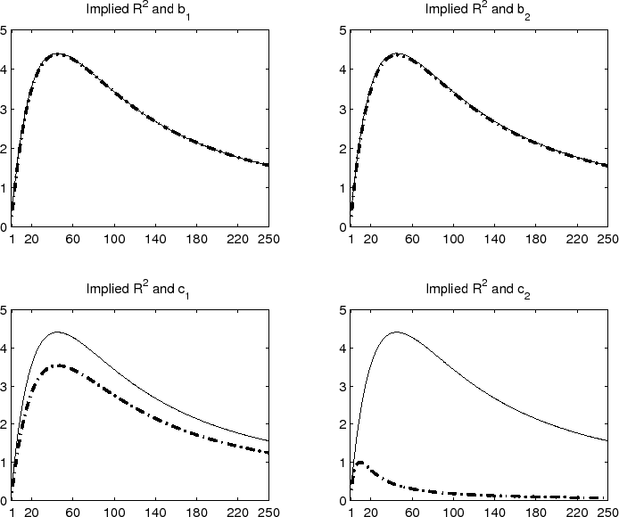
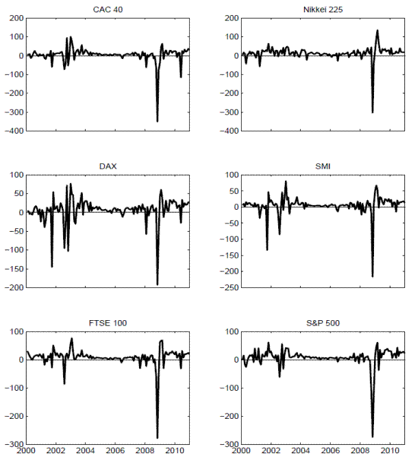
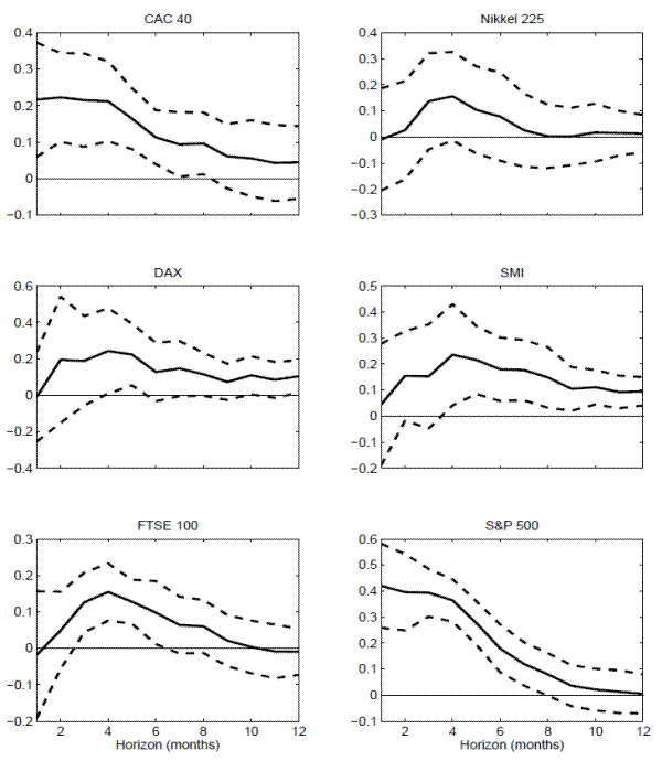
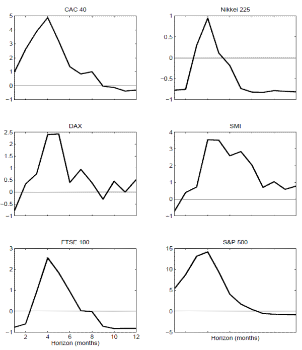
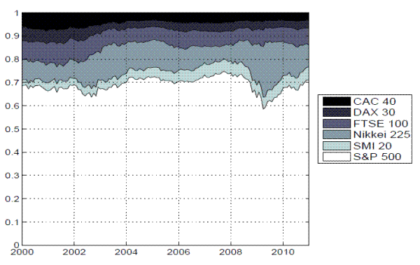
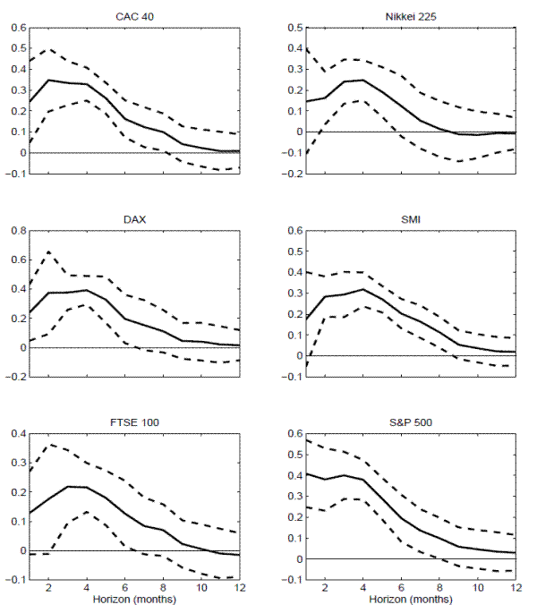
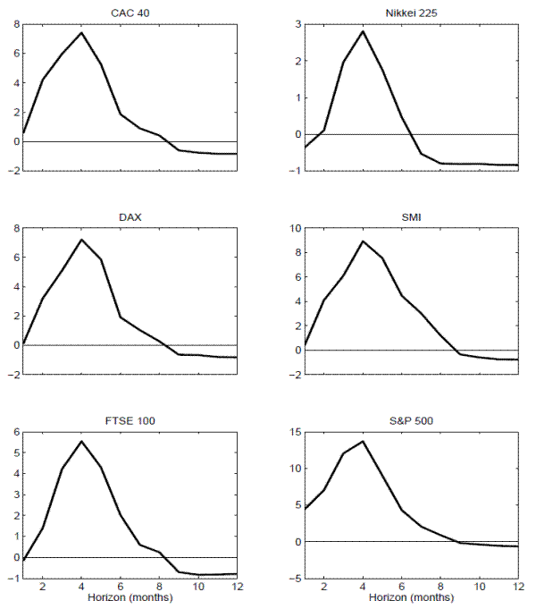
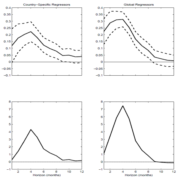
The top two panels show the estimated panel regression coefficients from regressing the returns on the individual country variance risk premia VRPti and the ``global'' variance risk premium VRPtglobal, respectively, reported in Table 6, together with two NW-based standard error bands. The bottom two panels show the R2's from the same two panel regressions. The regressions are based on monthly data from January 2000 through December 2010.
Figure 12: "Global" VRP Panel Regression  's
's
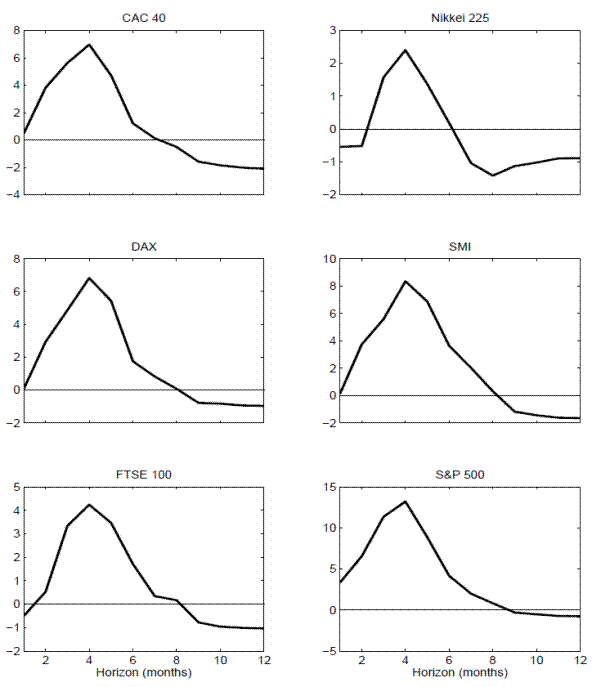
Figure 12 shows the adjusted R2's implied by the VRPtglobal panel regressions reported in the top panel in Table 5. The regressions are based on monthly data from January 2000 to December 2010.
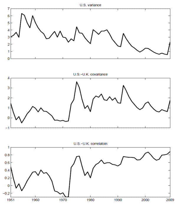
Figure 13 shows exponentially weighted moving average estimates for U.S. consumption growth variances, and covariances and correlations with U.K.
consumption growth. The estimates are based on annual total real consumption expenditures from 1951 to 2009, and a exponential smoothing parameter of ![]() =
=
![]() . The variances and covariances are both scaled by a factor of
. The variances and covariances are both scaled by a factor of ![]() .
.
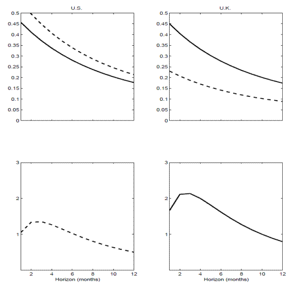
Figure 14 shows the implications from the calibrated stylized two-country general equilibrium model. The upper two panels plot the slope coefficients in the country specific regressions for each of the two countries based on the "local" VRP's (dashed lines) and "global" VRP (solid lines). The lower two panels show the implied panel regression ![]() 's based on the "local" (dashed line) and "global" (solid line) VRPs, respectively.
's based on the "local" (dashed line) and "global" (solid line) VRPs, respectively.