
FLOW AND STOCK EFFECTS OF LARGE-SCALE TREASURY PURCHASES: EVIDENCE ON THE IMPORTANCE OF LOCAL SUPPLY*
Keywords: Yield curve, quantitative easing, LSAP, preferred habitat, limits of arbitrage
Abstract:
The Federal Reserve's 2009 program to purchase $300 billion of U.S. Treasury securities represented an unprecedented intervention in the Treasury market and provides a natural experiment with the potential to shed light on the price elasticities of Treasuries and theories of supply effects in the term structure. Using security-level data on Treasury prices and quantities during the course of this program, we document a `local supply' effect in the yield curve-yields within a particular maturity sector responded more to changes in the amounts outstanding in that sector than to similar changes in other sectors. We find that this phenomenon was responsible for a persistent downward shift in yields averaging about 30 basis points over the course of the program (the "stock effect"). In addition, except at very long maturities, purchase operations caused an average decline in yields in the sector purchased of 3.5 basis points on the days when those operations occurred (the "flow effect"). The sensitivity of our results to security characteristics generally supports a view of segmentation or imperfect substitution within the Treasury market during this time.
1 Introduction
Do fluctuations in the supply of government debt affect Treasury yields? This possibility is generally ruled out under the expectations hypothesis and canonical arbitrage-free models of the term structure, but it can arise in models that account for imperfect asset substitutability or preferred-habitat investors. Theories consistent with these notions have existed informally for decades (e.g., Culbertson, 1957; Modigliani and Sutch, 1966), and they have recently received greater attention as researchers have begun to supply them with rigorous foundations, as in the models of Andres, Lopez-Salido, and Nelson (2004) and Vayanos and Vila (2009). Evaluating the significance of these mechanisms has the potential to inform modeling of the determination of bond and other asset prices. It is also important for a variety of policy issues, including the conduct of open market operations by central banks and the structure of debt issuance by governments.
We provide evidence on the response of the U.S. Treasury yield curve to the relative supply of Treasury securities by exploiting the natural experiment of the Federal Reserve's first round of Large Scale Asset Purchases (LSAPs) in 2009. Using new identification and estimation procedures based on security-level price and quantity data, we document what might be viewed as a relative-price anomaly in the Treasury market during this period, in the spirit of the evolving literature on market segmentation and supply shocks. In particular, we estimate a significant "local-supply" effect in the Treasury term structure: the yield on a given security fell in response to purchases of that security and securities of similar maturity. This response is conceptually distinct from-and more suggestive of market segmentation than-other mechanisms by which asset purchases might shift the yield curve, such as by changing the expected path of policy rates and inflation or changing the aggregate duration risk that market participants must bear. The $300 billion Treasury LSAP program, announced and implemented in the immediate aftermath of the financial crisis, is an ideal testing ground for a local-supply channel, not just because it represented a large (and largely unexpected) exogenous shock to the available Treasury supply, but also because it took place during a period of heightened risk aversion, which is precisely when the Vayanos-Vila (2009) theory predicts such a channel might be most operative. The security-level data allow us to examine how the scale of the local-supply effect varied across security characteristics such as maturity and liquidity and to gauge the degree of substitution across securities by estimating the cross-elasticities of their prices.
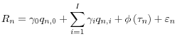
Within this framework, we distinguish two ways in which asset purchases might operate-through stock effects and through flow effects. "Stock effects" are defined as persistent changes in prices that result from movements along Treasury demand curves. To estimate stock effects, we model the cumulative change in each CUSIP's price between March 17, 2009 and October 30, 2009 (i.e., the cross section of Treasury returns) as a function of the total amount that the Fed purchased of that CUSIP and its potential substitutes.1 Because, over the life of the program, purchased amounts could have responded endogenously to price changes, we instrument these LSAP amounts with the purchased securities' characteristics prior to the announcement of the program. By removing our estimated stock effects from the actual cross section of Treasury prices as of the end of the LSAP program, we are able to construct a counterfactual yield curve that represents what interest rates might have looked like if the local supply channel had not been present. Meanwhile, "flow effects" are defined as the response of prices to the ongoing purchase operations and could reflect, on top of portfolio rebalancing activity due to the outcome of the purchases, impairments in liquidity and functioning that lead to sluggish price discovery. To estimate flow effects, we model the percentage change in each CUSIP's price on each day that purchase operations occurred as a function of the amount of that CUSIP and the amounts of substitute securities purchased on those days. This exercise is similar to the study of Brandt and Kavajecz (2004) on the response of yields to order-flow imbalances.
Our results suggest that, through the local-supply channel, the Fed's 2009 Treasury purchases reduced yields by an average of about 30 basis points over the life of the program (the stock effect) and led to a further 3 to 4 basis point decline in purchased sectors on the days when purchases occurred (the flow effect). We find that the stock effects were driven largely by the responses of less liquid securities, such as those that were several issues off the run. The flow effects were concentrated in securities with remaining maturities of less than 15 years that were eligible for purchase on a given day. Within this set, coefficients across various types of security characteristics and subperiods are quite robust, although we find that the flow effects were more persistent for off-the-run bonds, which is consistent with the stock effect being mainly driven by this category of assets.2 The sample of securities that were ineligible for purchase exhibits some instabilities in its flow effects, but those results are consistent with the results for eligible securities over the second half of the sample, by which time Treasury market conditions had substantially improved.
Both the stock- and flow-effect results provide support for preferred-habitat theories, as they demonstrate that Treasury rates at a given maturity are sensitive to the amount of privately held Treasury debt available around that maturity. Our results further indicate that, on the days when a security was eligible to be bought, purchases of securities with similar maturities had almost as large effects on its yield as did purchases of the security itself-that is, the cross- and own elasticities for flow effects were nearly identical-while purchases of maturities further away had smaller effects. This supports the view that Treasuries of similar maturities are close substitutes but that substitutability diminishes as maturities get farther apart, consistent with imperfect substitutability across the term structure. This set of results is also consistent with a series of papers, including Greenwood (2005), Gabaix, Krishnamurthy, and Vigneron (2007), Garleanu, Pedersen, and Poteshman (2009), Vayanos and Vila (2009), and Greenwood and Vayanos (2010b), where arbitrageurs transmit demand shocks for one asset to other assets, with the effects being the largest for assets that covary the most with the original asset-that is, for close substitutes. In addition, we find that certain types of Treasury securities exhibit greater evidence of segmentation, which is also supportive of preferred-habitat theories. For example, we generally reject equality of the own- and cross-elasticities in far-off-the-run Treasuries, suggesting that limits to arbitrage may play an even greater role among those securities. In other words, in less-liquid portions of the market, preferred-habitat investors' demand seems to dominate arbitrage activity during our sample.
Our paper fits within a growing literature studying the relationship between Treasury prices and quantities, including Bernanke, Reinhart, and Sack (2004), Engen and Hubbard (2005), Han, Longstaff, Merrill (2007), Krishnamurthy and Vissing-Jorgensen (2008), Greenwood and Vayanos (2010a, b), and Hamilton and Wu (2010). Much of this literature has relied on time-series studies of constant-maturity yields and aggregate characteristics of Treasury debt. Our panel-data approach offers a number of advantages over these methods. As noted above, the panel data allow us to get a granular picture of how supply effects differ across different types of securities and to estimate cross-elasticities of individual Treasuries with respect to their potential substitutes, procedures that are not generally feasible with aggregate data. In addition, the results of time-series studies may be affected by endogeneity problems typical of any estimated relationship between prices and quantities-indeed, these problems likely became more severe during the LSAP period as the Fed may have attempted to purchase securities that it viewed as underpriced. Security-level data allow us to build instrumental variables to address this endogeneity. Finally, analysis based on the aggregate characteristics of Treasury debt outstanding is not equipped to separate local supply effects from other mechanisms through which a change in supply may affect yields. By employing the prices of multiple securities and controlling for changes in the overall shape of the yield curve, we are able to isolate the local price responses to changes in the supply within specific, narrow maturity sectors.
The following section of the paper discusses the theory and notation behind our tests and positions our work within the existing theoretical and empirical literature. Section 3 develops our general empirical specification and gives an overview of our data. Section 4 presents our results, with sub-section 4.1 considering stock effects, and sub-section 4.2 considering flow effects. Section 5 concludes.
2 Theory and Evidence on the Effects of Treasury Supply
In this paper, we ask whether during the first LSAP program changes in the stock of Treasuries affected the yields on Treasuries in the specific sectors where purchases occurred-a possibility that we term the "local supply" effect. A number of previous studies (most explicitly, Greenwood and Vayanos, 2010b) have argued that Treasury supply may affect the term structure by changing the total quantity of duration risk that arbitrageurs must hold-when debt in public hands increases or shifts toward longer maturities, market participants are more exposed to shifts in interest rates and require higher premiums to bear this extra risk. This result, which we call the "duration effect," is distinct from the local-supply effect. The latter reflects relatively isolated movements within particular sectors of the yield curve, abstracting from any changes in the broader term structure that might have to do with duration exposure.
The local-supply effect falls within the category of relative-price anomalies of closely related assets, which, as pointed out in Gromb and Vayanos (2010), have only been documented sporadically, in part due to the rarity of natural experiments involving asset pairs with closely related payoffs. LSAPs provide precisely this type of natural experiment for the cross-section of Treasury securities.3 Gromb and Vayanos (2010) also note that these anomalies are difficult to reconcile with standard asset-pricing models. Indeed, most of the arbitrage-free models of the term structure of interest rates that have become common in the finance literature (e.g, Cox, Ingersoll, and Ross,1985) do not generally allow for effects of bond supply on interest rates, through either a duration channel or a local-supply channel.
On the other hand, the literature on the limits of arbitrage and preferred habitat has recently provided rigorous models that hold promise for explaining these anomalies. In particular, the theory that helps us to motivate the design of our tests is provided by Vayanos and Vila (2009) (V&V), as this is to the best of our knowledge the only formal model providing a mechanism by which demand and supply factors may affect yields locally. In the V&V theory, preferred-habitat investors have exogenously given demand curves for securities of each maturity, and they do not trade across different maturities. Meanwhile, arbitrageurs do trade across different maturities and render the term structure arbitrage-free in equilibrium by buying securities that are in low demand and selling those that are in high demand, but risk aversion prevents them from engaging in this process until expected returns are equated across securities. Thus, exogenous shocks to preferred-habitat demand can have effects on prices.
To be concrete, suppose that there are N distinct Treasury securities outstanding, indexed by n = 1,..., N. Let t![]()
![]()
![]() be
the remaining maturity of security n at time t and r
be
the remaining maturity of security n at time t and r![]()
![]()
![]() be its yield to maturity. Let the outstanding stock of Treasury debt available to
arbitrageurs be characterized by K "demand factors," b
be its yield to maturity. Let the outstanding stock of Treasury debt available to
arbitrageurs be characterized by K "demand factors," b![]() = (b
= (b![]()
![]() ... b
... b![]()
![]()
![]() ) and q
) and q![]() = (q
= (q![]() (1) ...q
(1) ...q![]() (N)) be the vector of loadings determining how the
k
(N)) be the vector of loadings determining how the
k![]() factor maps into the quantity of each security that arbitrageurs must hold.4 V&V assume that each security's demand-factor loadings depend only on its maturity, i.e. q
factor maps into the quantity of each security that arbitrageurs must hold.4 V&V assume that each security's demand-factor loadings depend only on its maturity, i.e. q![]() (n)=q
(n)=q![]() (m) whenever t
(m) whenever t![]()
![]()
![]() = t
= t![]()
![]()
![]() .5 In this case, their model generates a solution of the form
.5 In this case, their model generates a solution of the form
| (1) |
where r
V&V examine two polar cases of this model. In one extreme, when arbitrageurs are nearly risk neutral, the equilibrium value of each A![]()
![]()
![]() (t
(t![]()
![]()
![]() ) does not depend on any of the particular values of the factor loadings q
) does not depend on any of the particular values of the factor loadings q![]() (n), and it
is mainly determined by a term that can be interpreted as the average duration of the arbitrageurs' portfolio.6 Consequently, demand shocks have effects on the
entire term structure, including maturities that are distant from the particular sectors hit by those shocks. In the other extreme, when risk aversion is close to infinity and K is large, V&V suggest that the effects of a demand shock on the yields at maturity
t depends on how the shock affects quantities at that maturity-that is, A
(n), and it
is mainly determined by a term that can be interpreted as the average duration of the arbitrageurs' portfolio.6 Consequently, demand shocks have effects on the
entire term structure, including maturities that are distant from the particular sectors hit by those shocks. In the other extreme, when risk aversion is close to infinity and K is large, V&V suggest that the effects of a demand shock on the yields at maturity
t depends on how the shock affects quantities at that maturity-that is, A![]()
![]()
![]()
![]() (t
(t![]()
![]()
![]() ) is a function only of q
) is a function only of q![]() (n). Since each q
(n). Since each q![]() (n) itself is completely unrestricted (for example, it
may be discontinuous across t
(n) itself is completely unrestricted (for example, it
may be discontinuous across t![]()
![]()
![]() ), this means that demand shocks can have effects on yields that are local to particular maturities and do not, apart from these effects, change the term structure more
broadly. Between these two extremes, the solution for A
), this means that demand shocks can have effects on yields that are local to particular maturities and do not, apart from these effects, change the term structure more
broadly. Between these two extremes, the solution for A![]() (t
(t![]()
![]()
![]() ) is
complicated and intractable. However, as suggested by V&V's numerical investigations, we conjecture that A
) is
complicated and intractable. However, as suggested by V&V's numerical investigations, we conjecture that A![]() (t
(t![]()
![]()
![]() ) can be represented as a convex combination of the risk-neutral and infinitely-risk-averse outcomes. Therefore, we approximate A
) can be represented as a convex combination of the risk-neutral and infinitely-risk-averse outcomes. Therefore, we approximate A![]() (t
(t![]()
![]()
![]() ) as the combination of two distinct effects:
) as the combination of two distinct effects:
| (2) |
D
The distinction between duration effects and local-supply effects is important because yields can depend on the duration of investors' portfolios even when asset prices are determined solely by the behavior of arbitrageurs. For example, V&V also present a one-factor model, in which
preferred-habitat demand is constant and, consequently, r![]()
![]()
![]() is an affine function only of the short rate. Yet, even in this case, r
is an affine function only of the short rate. Yet, even in this case, r![]()
![]()
![]() still depends on the quantity of securities that are left in the hands of the arbitrageurs-the more supply the arbitrageurs are required to bear, in equilibrium, the greater the expected return they demand. Thus, finding a non-zero response of yields to supply
shocks is not necessarily evidence of preferred habitat per se. A more stringent test of the preferred-habitat hypothesis is whether local effects L
still depends on the quantity of securities that are left in the hands of the arbitrageurs-the more supply the arbitrageurs are required to bear, in equilibrium, the greater the expected return they demand. Thus, finding a non-zero response of yields to supply
shocks is not necessarily evidence of preferred habitat per se. A more stringent test of the preferred-habitat hypothesis is whether local effects L![]() are non-zero. Our tests below isolate local-supply effects, using LSAP purchases to identify exogenous shifts in the supply of each security available to investors.
are non-zero. Our tests below isolate local-supply effects, using LSAP purchases to identify exogenous shifts in the supply of each security available to investors.
While no study to date has specifically estimated the V&V model using observed data on Treasury supply fluctuations, Greenwood and Vayanos (2010b) have tested a number of qualitative hypotheses generated by V&V, and Kaminska, Vayanos, and Zinna (2011) have recently produced an estimated
version of that model using unobserved factors and TIPS prices. In both cases, the model fares well in explaining the aggregate pattern of Treasury yields. Yet neither of these studies examines the effects during the most recent financial crisis or any other period of heightened risk aversion.
Indeed, Greenwood and Vayanos (2010b) formulate all of their hypotheses in terms of the low-risk-aversion case-thus, they are essentially testing only for the presence of D![]() . Kaminska, Vayanos, and Zinna (2011), who include data through 2009 in their sample, note that their model generates large fitting errors during the crisis period and suggest specifically that this may be due to their assumption of constant risk
aversion.
. Kaminska, Vayanos, and Zinna (2011), who include data through 2009 in their sample, note that their model generates large fitting errors during the crisis period and suggest specifically that this may be due to their assumption of constant risk
aversion.
In addition, a number of studies (Bernanke, Reinhart, and Sack, 2004; Greenwood and Vayanos, 2010b; Hamilton and Wu, 2010) have found that various characteristics of the aggregate supply of Treasury debt are indeed correlated with the time-series behavior of the yield curve. In most of these
specifications, quantity shocks affect the term structure through essentially one supply factor proxied by some aggregate characteristic of the outstanding Treasury debt, such as average maturity. These studies have also typically restricted attention to rates at just one or a few points on the
yield curve. Despite the econometric challenges with regard to the possible endogeneity and persistence of the supply variables noted in the introduction, collectively-and together with anecdotal evidence on particular episodes-these studies suggest that supply plays a role. Still, it is difficult
to distinguish the two components of A![]() (t
(t![]()
![]()
![]() ) using aggregate
data alone. Thus, such studies cannot isolate local-supply effects.
) using aggregate
data alone. Thus, such studies cannot isolate local-supply effects.
Another type of evidence comes from event studies of particular episodes that have involved relatively large or rapid changes in Treasury supply.7 Our analysis of the first LSAP program fits within this tradition of exploiting "natural experiments," although with a different econometric methodology. One such episode is the Federal Reserve's attempt to decrease long-term yields relative to short-term yields in the early 1960s-termed "Operation Twist"-which involved the sale of short-term Treasury debt and the purchase of long-term debt. Although contemporaneous studies (Modigliani and Sutch, 1966; Ross, 1966; Holland, 1969) suggested that this program had little overall impact, a more recent reexamination by Swanson (2010) found statistically significant effects. Another interesting case is the Treasury Deparment's initiative to repurchase its long-term debt securities in 2000, which was similar to the Treasury LSAP program in mechanics, if not in scale. Bernanke, Reinhart, and Sack (2004), Longstaff (2004), and Greenwood and Vayanos (2010a) have argued that this program lowered long-term yields.8 While the results of these case studies are suggestive of local-supply effects' ability to rotate the yield curve, this type of finding could also be due to the effects of removing duration from the market.
In summary, although the existing evidence seems consistent with the possibility that changes in Treasury supply affect yields, it is difficult to get a precise idea of the magnitude of these effects, whether they reflect preferred habitat (in the sense of having local effects), or of how they vary with security characteristics because most previous analysis has been done at an aggregated level. No previous study that we know of exploits variation in quantities and prices for individual securities to account for timing issues (flow versus stock effects), endogeneity, substitutability across the term structure, and specific security characteristics.
3 Empirical Specification and a First Look at the Data
Our empirical work attempts to test for local-supply effects-that is, to characterize the functions L![]() that determine how shocks to quantities translate
into changes in yields on the securities that are directly affected by these shocks and in yields on nearby securities-using as a natural experiment the program to purchase up to $300 billion of Treasury coupon securities that the FOMC announced on March 18, 2009.
that determine how shocks to quantities translate
into changes in yields on the securities that are directly affected by these shocks and in yields on nearby securities-using as a natural experiment the program to purchase up to $300 billion of Treasury coupon securities that the FOMC announced on March 18, 2009.![]() 9 Our data consist of daily observations on the universe of outstanding nominal
Treasury coupon securities from March 17 through October 30, 2009 (the day after the purchases were concluded). To simplify the analysis, we exclude TIPS and securities with remaining maturities of less than 90 days, leaving us with an unbalanced panel of 204 CUSIPs. Our primary variables of
interest are the percentage price changes in each of these securities, measured at end-of-day, and the face values of the security-level quantities outstanding and amounts purchased under the LSAP program.10
9 Our data consist of daily observations on the universe of outstanding nominal
Treasury coupon securities from March 17 through October 30, 2009 (the day after the purchases were concluded). To simplify the analysis, we exclude TIPS and securities with remaining maturities of less than 90 days, leaving us with an unbalanced panel of 204 CUSIPs. Our primary variables of
interest are the percentage price changes in each of these securities, measured at end-of-day, and the face values of the security-level quantities outstanding and amounts purchased under the LSAP program.10
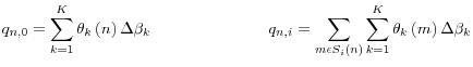
For each of the sample securities n, we partition the universe of outstanding securities into I+1segments, S![]() (n), that define buckets of "substitutes" for security n, where i = 0, ..., I. Note that we reserve i = 0 for the partition
consisting only of security n itself. This will allow for the possibility that shocks that affect the quantity of security n have effects on the yield of n that differ from the effects on all other securities (an
extreme form of the local-supply channel similar to the infinite-risk-aversion case in V&V). The dollar amount of substitutes for each security n purchased under the LSAP program in the i
(n), that define buckets of "substitutes" for security n, where i = 0, ..., I. Note that we reserve i = 0 for the partition
consisting only of security n itself. This will allow for the possibility that shocks that affect the quantity of security n have effects on the yield of n that differ from the effects on all other securities (an
extreme form of the local-supply channel similar to the infinite-risk-aversion case in V&V). The dollar amount of substitutes for each security n purchased under the LSAP program in the i![]() bucket is denoted by Q
bucket is denoted by Q![]() = S
= S![]()
![]()
![]()
![]()
![]()
![]()
![]() Q
Q![]() . Note that Q
. Note that Q![]()
![]() is the amount of security n itself purchased under the LSAP program. (We will refer to this as "own purchases.") We assume that the potential influence of dollar quantities purchased in a given sector may
depend inversely on the dollar amounts outstanding, say O
is the amount of security n itself purchased under the LSAP program. (We will refer to this as "own purchases.") We assume that the potential influence of dollar quantities purchased in a given sector may
depend inversely on the dollar amounts outstanding, say O![]() , in that sector or in other sectors. Thus we consider a normalized quantity variable q
, in that sector or in other sectors. Thus we consider a normalized quantity variable q![]()
![]()
![]() , where the normalization is a function of O
, where the normalization is a function of O![]()
![]() , ..., O
, ..., O![]()
![]()
![]()
![]()
Because coupon rates and maturities vary considerably across the universe of Treasury securities, we conduct our regressions in price space, rather than in yield space. Specifically, both our flow- and stock-effect regressions take the following general form:
 |
(3) |
where R
This empirical specification is consistent with the theory sketched in the previous section once we allow for quantity fluctuations at the individual-security level rather than at maturity level-i.e., we relax the V&V assumption that t![]() = t
= t![]() implies q
implies q![]() (n) = q
(n) = q![]() (m). This
specification allows for a higher level of disaggregation to exploit the richness of our security-level data. If we then specify
(m). This
specification allows for a higher level of disaggregation to exploit the richness of our security-level data. If we then specify
 |
(4) |
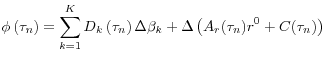
equation (3) is consistent with equation (1), once we substitute in equation (2) and further define
 |
(5) |
and
![\displaystyle L_{n} \left(\theta _{k} \right)=\gamma _{0} \theta _{k} (n)+\sum _{i=1}^{I}\left[\gamma _{i} \sum _{m\in S_{i} \left(n\right)}\theta _{k} (m) \right]](img33.gif) |
(6) |
where the changes (D) are computed over the observation frequency in our sample.12 In words, this specification assumes (a) that LSAP purchased quantities can be thought of as linear combinations of unobserved demand factors, (b) that movements in prices other than local-supply effects can be captured by smooth function of maturity, and (c) that the local-supply effects on prices are piecewise linear across the substitute buckets as we have defined them. Less formally, equation (3) simply conjectures that each security's price responds linearly to purchases of itself and its substitutes, after controlling for changes in the general configuration of the yield curve. Note that this specification does not require us to separately identify q and b or, for that matter, to specify the number of factors K.
The parameter g![]() reflects the local own-price elasticity of Treasury securities, while the parameters g
reflects the local own-price elasticity of Treasury securities, while the parameters g![]() ..., g
..., g![]() reflect the cross-elasticities of Treasury
security prices with respect to other Treasury securities. These latter elasticities depend on the degree of substitutability between different Treasuries, which in turn depends upon the ability of arbitrageurs to substitute across maturities and correct price discrepancies given their level of
risk aversion, capital constraints and market liquidity among other things.13 The own-price response g
reflect the cross-elasticities of Treasury
security prices with respect to other Treasury securities. These latter elasticities depend on the degree of substitutability between different Treasuries, which in turn depends upon the ability of arbitrageurs to substitute across maturities and correct price discrepancies given their level of
risk aversion, capital constraints and market liquidity among other things.13 The own-price response g![]() is of some interest, as its magnitude is indicative of the purchases' effects on the amounts by which an individual security's yield could deviate from those of similar securities (i.e.,
yield-curve fitting errors). The cross-responses, however, are likely to be much more important in terms of the aggregate level and term structure of interest rates. This is because the purchase of a particular securityaffects that security's yield alone through the g
is of some interest, as its magnitude is indicative of the purchases' effects on the amounts by which an individual security's yield could deviate from those of similar securities (i.e.,
yield-curve fitting errors). The cross-responses, however, are likely to be much more important in terms of the aggregate level and term structure of interest rates. This is because the purchase of a particular securityaffects that security's yield alone through the g![]() term, but it affects every security's yield through the applicable g
term, but it affects every security's yield through the applicable g![]() terms.
terms.
It remains to specify the partitions determining the substitute buckets S![]() (n). Although in principle we could choose the size,
number, and composition of these buckets in a variety of ways, a division into I = 3 buckets based on remaining-maturity ranges seemed to provide a good combination of parsimony and flexibility and allows us to test whether the degree of substitutability between
securities depends systematically on the difference between their maturities. In particular, for each security n, we define our most narrow substitute bucket (arbitrarily, i = 1) to include all securities having remaining maturities within two
years of security n's maturity-that is, S
(n). Although in principle we could choose the size,
number, and composition of these buckets in a variety of ways, a division into I = 3 buckets based on remaining-maturity ranges seemed to provide a good combination of parsimony and flexibility and allows us to test whether the degree of substitutability between
securities depends systematically on the difference between their maturities. In particular, for each security n, we define our most narrow substitute bucket (arbitrarily, i = 1) to include all securities having remaining maturities within two
years of security n's maturity-that is, S![]() (n) = {m: |t
(n) = {m: |t![]() - t
- t![]() |
|![]() 2; m ? n}. We refer to these securities as "near substitutes" for security n. The second bucket (i = 2), which we call "mid-substitutes" for n, includes all securities having remaining maturities that are between two and six years different from security n's. The third bucket (i = 3, or "far
substitutes") includes all securities having remaining maturities between six and fourteen years different from security n's. To compute q
2; m ? n}. We refer to these securities as "near substitutes" for security n. The second bucket (i = 2), which we call "mid-substitutes" for n, includes all securities having remaining maturities that are between two and six years different from security n's. The third bucket (i = 3, or "far
substitutes") includes all securities having remaining maturities between six and fourteen years different from security n's. To compute q![]()
![]()
![]() , we normalize by
the total amount of securities outstanding that have remaining maturities within two years of security n-that is, q
, we normalize by
the total amount of securities outstanding that have remaining maturities within two years of security n-that is, q![]()
![]()
![]() = Q
= Q![]()
![]()
![]() /(O
/(O![]()
![]() + O
+ O![]()
![]() ) .14
) .14
The characteristics of the purchased securities are summarized in Table 1 and Figure 1. Overall, purchases of nominal securities under the program included 160 unique CUSIPs, spanning remaining maturities of about two to thirty years. $300 billion represented about 3 percent of the total stock of outstanding Treasury debt and about 8 percent of the outstanding coupon securities as of the time of the announcement. Most purchases were concentrated in the 2- to 7-year sectors, although, as a percentage of total outstanding Treasuries within each sector, purchases across maturities were less concentrated. Coupon rates and vintages of securities purchased were roughly similar to the averages of all outstanding Treasuries. The maturity of securities bought was a bit longer than average, but the yields on purchased securities were notably higher than average-seemingly by too great a margin to be accounted for solely by their slightly longer maturities, especially given that a relatively high fraction (approximately 30 percent) of purchases were on-the-run issues, which generally have lower yields. This suggests that, consistent with contemporary commentary, the Desk deliberately purchased securities that were underpriced, a claim that we will illustrate more formally below.
Figure 2 shows the behavior of Treasury yields over the period of the program. After the initial announcement, medium- to long-dated yields fell by as much as 50 basis points, with yields in the 7-year sector declining twice as much as those in the 30-year sector. This is already suggestive of local-supply effects (or at least of the anticipation of such effects), since the duration effect of purchases should generally be expected to reduce longer-term yields by more, no matter where in the term structure the purchases occurred. In any case, the decline was short-lived-by early May most yields had returned to their pre-announcement levels, and they shot up further in June as the economic outlook improved. Although some of these increases reversed by October, most yields were still 20 to 40 basis points higher at the end of the program than they were before it started, and indeed they increased by the greatest amount in precisely the 5- to 10-year portion of the term structure where purchases were concentrated. These increases led some observers (e.g., Thornton, 2009) to conclude that the LSAPs had been ineffective in reducing interest rates. Of course, as we demonstrate below, such reasoning ignores other factors that may have been influencing yields over this period, including the possibility that the distribution of purchases itself was responding endogenously to relative changes in Treasury prices.
Another notable pattern over this period-and one that may itself have been due in part to the Treasury LSAP program-is the improvement in liquidity in the Treasury market. Traders had pointed to reduced liquidity as an important factor putting upward pressure on some yields in the weeks leading up to the introduction of the program. As Table 2 illustrates, almost every measure of liquidity improved between the first and second halves of the program's life. Average trading volumes increased by 20 percent, the yield premium paid for on-the-run 10-year note over off-the-run securities with comparable remaining maturities fell by a quarter, and failures to deliver securities into repurchase agreements on Treasuries declined by 80 percent. The final column of the table shows the average residuals that result from fitting a smooth curve, using the functional form proposed by Svensson (1994), to the cross-section of yields on each day. These yield curve "fitting errors," which can be interpreted as a measure of unexploited price discrepancies, declined by about half between the two sub-periods.15
4.1 Stock Effects
Specification Details
By "stock effects" we mean the impact that the LSAP program had on prices by permanently reducing the total amount of Treasury securities available for purchase by the public within a given sector. Of course, expectations of such effects should have been impounded into Treasury prices as soon as the market became aware of the program, before any purchases took place-presumably, this mechanism accounted for much of the 25 to 50 basis point drop in Treasury yields on the day the program was announced.16 Thus, it is crucial to account for expectations when measuring stock effects. However, we note that changes in investor expectations matter only prior to the conclusion of the program. In other words, while there may be temporary price fluctuations reflecting changing expectations of future purchases, these expectations become irrelevant once the total actual amounts and distribution of purchases is revealed. Thus, all else equal, the difference in price changes across two securities between the time the program was announced and the time it was concluded should depend only on the relative amount of each security that was actually purchased over the life of the program.
Some previous event studies of LSAPs, such as Gagnon, Raskin, Remache, and Sack (2010), have tried to identify their effects by looking at the reaction of prices within a specific time-window around important announcements. The difficulty with this approach (apart from specifying the appropriate window length) is that it relies solely on changes in expectations of purchases that occur within the windows-if market participants had some expectation of purchases prior to the windows, or if they changed their expectations any time outside the windows, or if they waited until purchases actually occurred to fully impound their effects, the event study will not capture the true effects of the program. Instead, our approach relies solely on cross-sectional variation for identification and is therefore less susceptible to this sort of timing critique.
With this in mind, our regressions for the stock effects use the cross section of total price changes for all nominal Treasury coupon securities between March 17 and October 30, 2009 (the day before the first LSAP announcement and the day after the last purchase). We seek estimates of the
coefficients g in equation (3). We assume that the maturity-dependent yield-curve movements f(t![]() ) are
sufficiently smooth that they can be well approximated by a second-order polynomial. In addition to the duration effects of LSAP purchases, these terms account for possible secular changes in the slope and curvature of the yield curve during our period that could have resulted from macroeconomic
conditions and new Treasury issuance. In the cross-section analysis, we do not use the mid- or far-substitute categories because of the high degree of collinearity, especially given our inclusion of the remaining maturity variables. Thus, equation (3) reduces to a linear regression of returns on
own and near substitute purchases, with linear and quadratic terms for maturity as control variables.
) are
sufficiently smooth that they can be well approximated by a second-order polynomial. In addition to the duration effects of LSAP purchases, these terms account for possible secular changes in the slope and curvature of the yield curve during our period that could have resulted from macroeconomic
conditions and new Treasury issuance. In the cross-section analysis, we do not use the mid- or far-substitute categories because of the high degree of collinearity, especially given our inclusion of the remaining maturity variables. Thus, equation (3) reduces to a linear regression of returns on
own and near substitute purchases, with linear and quadratic terms for maturity as control variables.
However, there is an obvious danger of endogeneity in our exercise-if the Fed was deliberately targeting securities that were underpriced, purchases may have been higher among issues whose yields rose the most during the life of the program. To control for this possibility, we use two-stage least squares. In the first stage, we instrument the LSAP purchase amounts of each security using information about the security's characteristics available before the program was announced. Specifically, our instruments are: the fitting errors from a Svensson yield curve estimated on March 17; the percentage of each security held by the Fed in the SOMA portfolio as of March 17; a dummy variable for whether the security was on-the-run as of March 17; and a dummy variable indicating whether the security had less than two years remaining until maturity on March 17.
Table 3 reports the results of a regression of actual LSAP purchases (as a percentage of the par value of each security outstanding) on these instruments and the remaining-maturity quadratic terms. All of the coefficients are statistically significant at the 1 percent level. The coefficients on the maturity variables suggest that purchases depended strongly on remaining maturity and, controlling for other factors, peaked around the twelve-year sector (in percentage-of-issue terms). The yield-curve fitting errors have a positive sign, confirming the conjecture that the Desk tended to purchase securities that were underpriced (i.e., had higher yields) than other securities with similar remaining maturities. The Fed was less likely to purchase securities that it already owned, presumably reflecting its self-imposed ownership limit of 35 percent of each issue, and, as was suggested in Table 1, was more likely to purchase on-the-run than off-the-run issues. Finally, the Fed purchased virtually nothing with maturity of less than two years.17
Two further transformations are required for our instruments. First, the specification presented in Table 3 is probably the right one-the Fed likely determined how much of each CUSIP to buy as a fraction of the amount outstanding of that CUSIP. However, in our second-stage regressions, we want
to use the quantity normalized by the amount outstanding in the relevant sector-Q![]()
![]() /(O
/(O![]()
![]() + O
+ O![]()
![]() ), not Q
), not Q![]()
![]() /O
/O![]()
![]() . We thus use q
. We thus use q![]()
![]() as the dependent variable in the first stage but, to maintain consistency,
we weight each of our four security-level instruments by O
as the dependent variable in the first stage but, to maintain consistency,
we weight each of our four security-level instruments by O![]()
![]() /(O
/(O![]()
![]() + O
+ O![]()
![]() ). Second, purchases of substitutes are subject to the
same endogeneity concerns as own purchases, so we also instrument for q
). Second, purchases of substitutes are subject to the
same endogeneity concerns as own purchases, so we also instrument for q![]()
![]() . As instruments, we simply average each of the four instrumental variables listed above over the bucket of near substitutes for each security, weighting by amounts outstanding. We include both the security-specific and sector-average instruments in both of our
first-stage equations. In the second-stage regression, we use instrumented purchases from the first stage as independent variables and the cumulative changes in Treasury prices as the dependent variable.
. As instruments, we simply average each of the four instrumental variables listed above over the bucket of near substitutes for each security, weighting by amounts outstanding. We include both the security-specific and sector-average instruments in both of our
first-stage equations. In the second-stage regression, we use instrumented purchases from the first stage as independent variables and the cumulative changes in Treasury prices as the dependent variable.
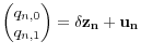
In summary, our baseline two-stage system takes the form
 |
(7) |
| (8) |
where R![]() is security n's gross return, z
is security n's gross return, z![]() is the vector of instruments, hats indicate instrumented values from the first stage, and t
is the vector of instruments, hats indicate instrumented values from the first stage, and t![]() is the remaining maturity as of March 17. Because we are using a cross section, we exclude securities that matured or were issued while the program was in progress, leaving us with 148 observations.
is the remaining maturity as of March 17. Because we are using a cross section, we exclude securities that matured or were issued while the program was in progress, leaving us with 148 observations.
We do not explicitly control for the Federal Reserve's purchases of other assets-agency debt and MBS-during the LSAP period. In this choice, we follow the previous literature in this area, which almost exclusively confines attention to the supply of Treasuries when studying the effects of debt supply on yields. (As a more practical matter, the data necessary to control for MBS purchases in our framework are not publicly available.) Note that in order for the omission of these other asset purchases to bias our results, they would have to be cross-sectionally correlated with the pattern of Treasury purchases and yield changes, and there is no particular reason to suspect this.18 Similarly, an identifying assumption for our regressions is that LSAP purchases were cross-sectionally uncorrelated with other changes in Treasury supply over the period of the program (after controlling for maturity).
Finally, in order to examine how our results vary with liquidity and other security characteristics, we want to allow the second-stage coefficients to differ across security groups. In particular, we will divide the sample by security type, maturity, and vintage. The small number of observations
makes running separate regressions on each of these groups problematic, and, moreover, there is no particular reason to think that the first-stage equation or the second-stage coefficients on t![]() should differ across them. Therefore, we continue to run all of our regressions on the full sample but, in the second stage, we allow the coefficients on own and substitute purchases to differ across the groups:
should differ across them. Therefore, we continue to run all of our regressions on the full sample but, in the second stage, we allow the coefficients on own and substitute purchases to differ across the groups:
| (9) |
where g indexes the groups. We perform this estimation by interacting
![]() and
and
![]() with dummy variables that divide the sample into mutually exclusive subsamples-notes vs. bonds, short vs. long maturities, and near-on-the-run vs. far-off-the-run
securities.
with dummy variables that divide the sample into mutually exclusive subsamples-notes vs. bonds, short vs. long maturities, and near-on-the-run vs. far-off-the-run
securities.
Results
The results of the second-stage regressions, with gross returns as the dependent variable, are presented in the first column of Table 4. Both own purchases and near-substitute purchases have positive and statistically significant effects on returns, although the effects of own purchases appear to be considerably larger. However, a likely source of misspecification in these results is that, if individual yield curve fitting errors are not persistent, the prices of securities with positive fitting errors would tend to fall relative to other securities and those with negative fitting errors would tend to rise, even in the absence of LSAP purchases-in other words, initial fitting errors might be correlated with the second-stage error term. In addition, there may be other information embedded in the initial prices of securities that reflects expectations of future returns. To control for these possibilities, we run an alternative specification in which we include the initial percentage price fitting error and the initial log price as exogenous regressors. (We also include both variables in the first-stage regression.) These results are shown in the second column. Both of the new regressors are highly significant, arguing for their inclusion. In this specification, the estimated values of both the own and near-substitute coefficients fall notably, but they retain their basic qualitative pattern and statistical significance.
The coefficient of 0.07 on substitute purchases suggests that buying 1 percent of a security's near substitutes (about $10 billion for the average security in our sample) increased the price of that security by 0.07 percent. For a typical ten-year Treasury, with a modified duration of 7 years, this translates into a yield change of -1 basis point. The coefficient on own purchases implies that if the same dollar amount had been used entirely to purchase a single security, the price of that security would have risen by 0.61 percent; again taking the ten-year Treasury as representative, its yield would have fallen by about 9 basis points. The strong statistical and economic significance of these results supports the existence of local-supply effects. In addition, the smaller magnitude of the substitute coefficient than the own coefficient suggests imperfect substitution across securities within the same sector.
We next break our data into subsamples, using the interactive-dummy technique described above. In particular, we consider possible differences between notes and bonds, securities with relatively long maturities versus those with shorter maturities, and recently issued securities versus older issues. The distinction between notes and bonds is potentially interesting largely as a proxy for other security features. The bonds all had original maturities of 30 years and most of them are old issues that tend to have much smaller trading volumes and lower liquidity than notes, as well as higher coupons.19 To distinguish longer and shorter maturities, we split the sample at the middle of the yield curve, 15 years. (About 90% of the securities in our sample were in the less-than-15-year sector.) To distinguish securities of recent versus older vintage, we split the sample in to securities that are more than five issues off the run and those that are less than six. In all of these regressions, we include controls for initial prices and fitting errors, given the better fit of that model in the pooled regression above, although the qualitative results are robust to these controls.
Table 5 presents the results for these various subsamples. The magnitude and significance of substitute purchases vary across the subsamples, but the differences are not economically large and we cannot reject that any of these coefficients are equal to the value of 0.07 presented in the previous table. The effects of own purchases are only statistically significant among the subsamples of bonds, far-off-the-run securities, and shorter-maturity securities. We note that the results split by maturity support the claim that we have in fact identified local-supply effects rather than duration effects, since the latter should generally be increasing in maturity.
However, we cannot reject that the own coefficients are the same for notes and bonds and for short and long maturities. The one instance in which we do find significant differences in the own coefficients is when we split according to security vintage-purchases of far off-the-run securities have
large and highly significant effects, while purchases of near on-the-run securities have none at all. Consistent with the significance of this difference, this specification also fits the data better in terms of adjusted R![]() than any of the others we tried. Proximity to on-the-run status is a proxy for liquidity, suggesting that a great deal of the local-supply stock effect of the LSAP program was due to the relative illiquidity of the securities purchased.
than any of the others we tried. Proximity to on-the-run status is a proxy for liquidity, suggesting that a great deal of the local-supply stock effect of the LSAP program was due to the relative illiquidity of the securities purchased.
Counterfactual yield curve
To summarize the local-supply stock effects of the LSAP program, we construct a counterfactual yield curve using the best-fitting results presented in Table 5. In particular, by using the actual value of purchases of each security and its near substitutes, together with the coefficients for the appropriate sub-sample, we compute the estimated amount by which the price of that security changed as a result of LSAP purchases. Subtracting this value from the actual price at the end of the program gives the counterfactual price of each security that would have obtained if the LSAPs had not occurred (holding other effects on the slope and curvature of the yield curve constant). The corresponding yields are shown as the squares in Figure 3, with + and - signs indicating the 95 and 5 percent confidence bounds for each security. (These are calculated by finding the confidence interval around the fitted value of each security's price and then transforming that value into a yield.) The dots in the figure show the actual yields on October 30, 2009. The difference between the squares and dots marks represents the local-supply stock effects of the LSAP program on yields to maturity. The peaks in the squares around the 7-, 13- and 17-year maturity sectors are clear illustrations of the local effects.
For almost all securities, the counterfactual yields lie significantly above the actual yields. The largest effect on average appears to be at the very short end of the curve, but these responses are estimated with some noise and are driven by the very short duration of securities in that region. (The estimated effect on prices at the short end is very small.) Beyond maturities of about a year, the largest effects are around horizons of about 6 to 8 years and 11 to 14 years, consistent with the relatively high proportion of securities that were purchased in these sectors and the relatively high coefficients on off-the-run securities, which dominate those sectors. Again, we see very little response at the long end of the yield curve, supporting our interpretation of these estimates as local-supply effects. Averaging over all securities, we estimate that the local effects of LSAP purchases shifted the level of yields by about 30 basis points, for an average elasticity of about 1 basis point for every $10 billion bought.
To see these effects in another way, we obtain smooth zero-coupon yields by fitting prices to a Svensson yield curve, with securities weighted by their inverse duration as in Gurkaynak, Sack, and Wright (2007). The 5 percent and 95 percent confidence bands around the counterfactual prices are treated in the same way. These results are shown, together with the actual Svensson curve on October 30, 2009, in Figure 4. The difference between the solid thin and thick lines represents the smoothed local-supply stock effects of the LSAP program on zero-coupon yields. From this picture, we can see that the effects were negative and statistically significant over all maturities of less than about 25 years. Indeed, over horizons of about 5 to 15 years, the shift in the yield curve is roughly uniform at 20 to 30 basis points. (The positive response of zero-coupon yields at the very long end of the yield curve is consistent with the observation, from Figure 3, that yields to maturity at that horizon were essentially unaffected by the local-supply effects of the program.)
4.2 Flow Effects
In this section, employing a panel, we test whether Treasury LSAP purchases had effects on Treasury prices around the times when purchases occurred in the sectors where they occurred. Again, we define such responses as the "flow effects" of the program.
Some additional detail on the mechanics of the individual purchase operations may be useful in interpreting the flow-effect results. The first operation under the Treasury LSAP program was conducted on March 25, 2009. Purchases continued at a pace of about $10 billion per week over the subsequent five months but gradually slowed beginning in August to minimize any potential disruption that might have resulted from a sudden closing of the program. In total, there were 57 purchase operations of nominal Treasury securities. The logistics of these operations were as follows. Every-other Wednesday, the Open Market Desk at the Federal Reserve Bank of New York ("the Desk") announced the broad maturity sectors in which it would be buying over the subsequent two weeks and the days on which it would be conducting these operations. These maturity sectors included securities spanning ranges of between one year (at the short end of the yield curve) and 13 years (at the long end), with an average range of about four years. Auctions took place from Monday of the first week through Friday of the second week and typically settled on the following day.20 At 10:15 on the morning of each auction, the Desk published a list of CUSIPs that were eligible for purchase, which generally included nearly all securities in the targeted sector, and began accepting propositions from primary dealers.21 Propositions included the amount of each CUSIP that the dealer was willing to sell to the Desk and the price at which it was willing to sell. At 11:00 AM, the auction closed. The Desk then determined which securities to buy from among the submitted bids based on a confidential algorithm and published the auction results within a few minutes. Market participants were not aware in advance of the total amount to be purchased or of the distribution of purchases across CUSIPs. Notably (consistent with standard market practice) settlement of the winning bids did not occur until the following day, so that dealers could, in principle, have submitted propositions for securities they did not own and, if they won, purchased these securities to settle the next day with the Desk.
Because the sectors of purchase operations were announced in advance and both the list of CUSIPs and the total size of each operation were fairly predictable, one might expect that examining yield changes as function of contemporaneous purchases would reveal no statistically significant responses. However, within the list of eligible securities, the particular CUSIPs that were purchased and the amounts of these purchases were not known in advance to the market, so yield differentials could have emerged on the days of purchases between securities that were purchased and those that were not. In addition, under limits to arbitrage, even perfectly anticipated changes in supply could have effects on prices when they occur, as shown by Lou, Yan, and Zhang (2010) in the case of Treasury auctions. The tests below will include both of these phenomena. Market-microstructure, settlement, and other technical factors could also cause yields to move in response to supply fluctuations, even if those fluctuations are predictable. However, in this case, we would expect the effects to reverse quickly. We therefore also examine price movements on the day after purchase operations to test whether the effects are persistent, which would favor more fundamental explanations such as preferred habitat.
Specification Details
Having panel data leads us to make four notable adjustments to the specification we used in the cross-sectional stock-effect estimation above. First, to control for duration effects and other shifts to the overall term structure (i.e., f(t![]() )) at a daily frequency, we use time-dummies. This is less restrictive than it may at first appear because individual purchase operations were conducted within fairly
small maturity ranges (about 4 years, on average). Within these ranges, daily slope and curvature shifts are generally quite small. Second, we include security-level fixed effects to control for the possibility, suggested in the stock-effect results, that some securities may have experienced higher
returns over the period, independent of local-supply and duration effects (perhaps as a result of decaying fitting errors). Third, we do not use instrumental-variables estimation when measuring flow effects because, at a daily frequency, the Fed is unlikely to have responded meaningfully to price
changes in specific securities or sectors. Finally, we are able to consider our mid- and far-substitute buckets in the flow-effect regressions because the greater sample size and observation heterogeneity reduces the multicollinearity problem.
)) at a daily frequency, we use time-dummies. This is less restrictive than it may at first appear because individual purchase operations were conducted within fairly
small maturity ranges (about 4 years, on average). Within these ranges, daily slope and curvature shifts are generally quite small. Second, we include security-level fixed effects to control for the possibility, suggested in the stock-effect results, that some securities may have experienced higher
returns over the period, independent of local-supply and duration effects (perhaps as a result of decaying fitting errors). Third, we do not use instrumental-variables estimation when measuring flow effects because, at a daily frequency, the Fed is unlikely to have responded meaningfully to price
changes in specific securities or sectors. Finally, we are able to consider our mid- and far-substitute buckets in the flow-effect regressions because the greater sample size and observation heterogeneity reduces the multicollinearity problem.
Our flow-effect regressions are thus the following analogue of equation (8):
 |
(10) |
where a![]() is a security-specific fixed effect, d
is a security-specific fixed effect, d![]() is a time dummy, e
is a time dummy, e![]()
![]()
![]() is an error term, and we have added time subscripts to the return and quantity variables to indicate price changes and quantities
purchased on specific days. Note that, in addition to accounting for the issues mentioned above, the fixed effects and daily time dummies enable us to control for a variety of occurrences, such Treasury auctions, that could shift relative demand and supply in a small portion of the nominal coupon
market.
is an error term, and we have added time subscripts to the return and quantity variables to indicate price changes and quantities
purchased on specific days. Note that, in addition to accounting for the issues mentioned above, the fixed effects and daily time dummies enable us to control for a variety of occurrences, such Treasury auctions, that could shift relative demand and supply in a small portion of the nominal coupon
market.
Because the maturity sectors within which securities were purchased on any given day were announced in advance, we may expect that securities within those sectors might have reacted differently to the purchase operations than securities that were outside the purchased sectors. To examine this possibility, we split the sample into (1) observations of securities on days when those securities were within the announced purchase sectors (defined as "eligible" securities) and (2) observations of securities on days when purchases took place in different sectors (defined as "ineligible"). These subsets are mutually exclusive and exhaustive within the set of days on which purchases took place, though the same CUSIP can appear in both groups on different days.
Finally, it is possible that, because of settlement lags or other microstructure issues, the effects of purchases are not fully realized until the day after they occur. Moreover, we are interested in the persistence of the flow effects and would like to test for possible reversion in prices in the days following the operations. To check for these possibilities, we also look at returns on the days after purchase operations by running regressions of the form
 |
(11) |
where R![]()
![]()
![]()
![]() is the return the day after the operation.
is the return the day after the operation.
Results for Eligible Securities
We begin by analyzing the results for the eligible securities. In Table 6 we report the baseline results. Initial tests suggested that the coefficients differed for securities with very long remaining maturities, so we report a sample split at the midpoint maturity of 15 years. Focusing on the first column of the table, which pertains to eligible securities with remaining maturities of less than 15 years, the coefficient of 0.276 on own purchases implies that, on average, purchasing $1 billion of Treasuries increased the price on the securities purchased by about 0.02 percent; for a representative 10-year security with a duration of 7 years, this translates into a yield decrease of about 0.3 basis points per billion dollars purchased. On the days when a security was eligible to be bought, purchases of its "near substitutes" had almost as large effects on its yield as did purchases of the security itself, pointing to a very high degree of substitutability among these securities.22 However, the coefficients are somewhat smaller for mid-substitutes, consistent with our hypothesis that local effects should die off as maturity distance increases. Applying the aggregate coefficients to averages of the dependent variables, and multiplying by the average inverse modified duration, we find that the typical effect of each operation was on the order of -3.5 basis points for the sector being purchased. (Operations averaged about $5 billion in size.) The second column of Table 6 shows that these results did not generally hold for issues with maturities greater than 15 years.
In the remainder of this section, we focus only on securities with less than 15 years to maturity, because that is where the great majority of purchases occurred. Within this sub-sample, Table 7 further splits the data into various groups to examine the consistency of the coefficients. First, we split the sample into purchases that occurred during the first half of the LSAP program (March 25 - July 6) and those that occurred during the second half (July 7 - October 29). As noted earlier, liquidity in the Treasury market was substantially better during the second half of the sample. Thus, if the price responses to LSAP purchases were due to impediments to market clearing and price discovery resulting from poor market functioning, we would expect the results to be substantially weaker in the second sub-sample. The first two columns of the table show that there is no evidence of this among securities that were eligible for purchase-the coefficients are nearly identical for the two sub-periods and are very close to the pooled results reported in the first column of Table 6.
The middle columns of Table 7 split the sample into notes and bonds. Again, the results for the subsamples are generally similar to each other and to the results presented in Table 6 in terms of sign, magnitude, and significance. Similarly, the last two columns, which split the sample into securities more than five and less than six issues off the run, show no major differences. The modest exception is that the samples of bonds and far-off-the-run securities show somewhat smaller effects of substitute purchases. This is consistent with weaker substitutability among these relatively illiquid securities.
Results for Ineligible Securities
Table 8 displays results for securities that were ineligible for purchase, comparably to Table 6. In the aggregate, these responses display little economic or statistical significance. However, a further split of this sample reveals a more interesting pattern. Namely, as shown in Table 9, the coefficients on all of the substitute purchases are negative in the first half of the sample and positive in the second half. (As above, we focus here on the less-than-15-year sector of the yield curve, where most purchases took place.) During the second half of the sample, the coefficients on near- and mid-substitute purchases are close to those for the eligible sample, as we would expect given that there was generally little qualitative difference between eligible and ineligible securities.23 Thus, the first half of the sample for the ineligible securities is the puzzling piece of the data. It seems possible that the differences between eligible and ineligible securities during this time may have had to do with the liquidity impairments in the market noted above, although the exact mechanism that would result in this pattern is unclear. Another possible explanation is that dealers initially anticipated being able to sell more to the Fed than they actually were able to sell and thus unloaded portions of their inventories (including securities that had not been eligible) in the wake of LSAP operations in order to maintain portfolio targets. Such an effect would likely have dissipated by the second half of the sample, as participants learned the pattern of the Desk's operations.
Table 10 shows that the basic patterns described above for the eligible and ineligible securities in the first and second halves of the sample do not depend on the liquidity characteristics of the securities considered, as proxied by the split into notes and bonds. (Again the bonds are largely far-off-the-run issues that trade infrequently.) The coefficients on purchases of eligible securities are almost always positive and significant, with fairly consistent magnitudes,24 while the negative coefficients for ineligible securities in the first half of the sample appear irrespective of security type.
Results for the Day After Purchases
Table 11 turns to the question of what happened on the days after LSAP operations took place. For comparison, the sample breakdown and independent variables are the same as those used in Table 10, but now the dependent variable is the security return on day t+1. Consider first the sample of eligible securities, presented in the left-hand sets of columns. For eligible note securities, prices almost uniformly reversed the increases they experienced on the days of purchases-the coefficients are of roughly similar magnitudes to those reported in the top panel of Table 10, but they are all negative (although they are not individually significant in the second half of the sample). This suggests that the local-supply flow effects among notes were short-lived. On the other hand, for eligible bonds (which, again, tend to be less liquid) prices actually increased further on the days after purchases. Indeed, tests using price changes on subsequent days (not shown) suggest that the effects of LSAP purchases on these bonds may have never fully reversed, perhaps contributing to the large stock effect observed in this category.25
These results suggest that even anticipated purchases can have significant local effects on prices in some circumstances. A brief spike and retreat in prices, such as occurred among notes, can be explained by settlement, clearing, and rebalancing frictions. But a persistent increase in prices following a purchase that was announced in advance would seem to call for a more substantial explanation, such as preferred habitat. That this pattern is evident among the less-traded securities further supports the idea that such a mechanism may be at work, as in less-liquid portions of the market, preferred-habitat investors' demand might dominate arbitrage activity.
Finally, turning to the day-after results for ineligible securities, the coefficients for notes are similar to those in the eligible sample, again suggesting good substitutability (as we would expect) across these groups. The sign and significance of the coefficients on ineligible bonds do not show a clear pattern, but the coefficient magnitudes are small compared to most of the other samples we have reported. In general (also taking into account Table 10), it does not appear that the prices of ineligible bonds increase with their eligible counterparts following purchases. This is somewhat puzzling but could again be consistent with the relatively weak liquidity for these securities.
Robustness to Error Correlation
Tables 12 and 13 present results for the baseline samples and key subsamples using clustered standard errors. Because it seems plausible that the regression errors are correlated across maturity, we allow for clustering within one-year maturity buckets for each security. This adjustment does not alter any of our results, either for the baseline breakdown or for the subsamples-indeed, in some cases the clustered standard errors are smaller than in the baseline case (suggesting negative correlation within clusters). We also clustered by security type (not shown) and did not observe any notable differences with the results reported above.
5 Conclusion
In this paper, we have used CUSIP-level data to estimate the local flow and stock effects of the Federal Reserve's 2009 program to purchase nearly $300 billion of nominal Treasury coupon securities. We find that both the flow and stock effects were statistically and economically significant. Specifically, we estimate that the average purchase operation temporarily reduced yields by about 3.5 basis points in the sector of the purchase and that the local-supply effects of the program as a whole shifted the yield curve down by up to 30 basis points, with both effects concentrated at medium maturities. These are distinct from any effects the program may have had through other channels, such as lowering the expected path of short-term rates and removing duration from the market.
These results provide support for preferred-habitat and portfolio-balance theories of the term structure. Consistent with such theories, we find that: withdraws of Treasury supply decrease yields by an economically meaningful amount; these decreases are generally biggest for the specific securities being bought and for securities of similar maturities but smaller for securities with much different maturities; particularly for stock effects, the discrepancies between own purchases and substitute purchases are larger among less-liquid securities (off-the-run bonds); also among off-the-run bonds, the flow effects are persistent, suggesting that they are not just due to short-run rebalancing or microstructure-related distortions.
Our study is the first to specifically consider local-supply effects on the yield curve, but the overall magnitudes of our stock-effect estimates are roughly comparable to what would be implied by Treasury price elasticities found in some other research, such as Kuttner (2006). As far as we are aware, no other study has estimated flow effects controlling for different degrees of substitution (as we have defined them). It is perhaps surprising that these effects should be so large in most subsamples, given that most details of the purchases were announced in advance. There is certainly room for additional work to understand whether similar effects hold in other markets and in other periods and, if so, exactly what mechanisms are behind them.
Finally, we have motivated the study of the first LSAP period, which was a time of poor liquidity and high risk aversion, as a promising environment to test for local-supply effects, but we caution that those same features could make extrapolation of our results to other situations problematic. How local supply effects differ across risk and liquidity regimes is an interesting area for future research and could further illuminate the factors that influence pricing and functioning in the Treasury market.
Figure 1. Maturity Distribution of Nominal Treasury LSAP Purchases - Billions of Dollars - Percentage of Sector
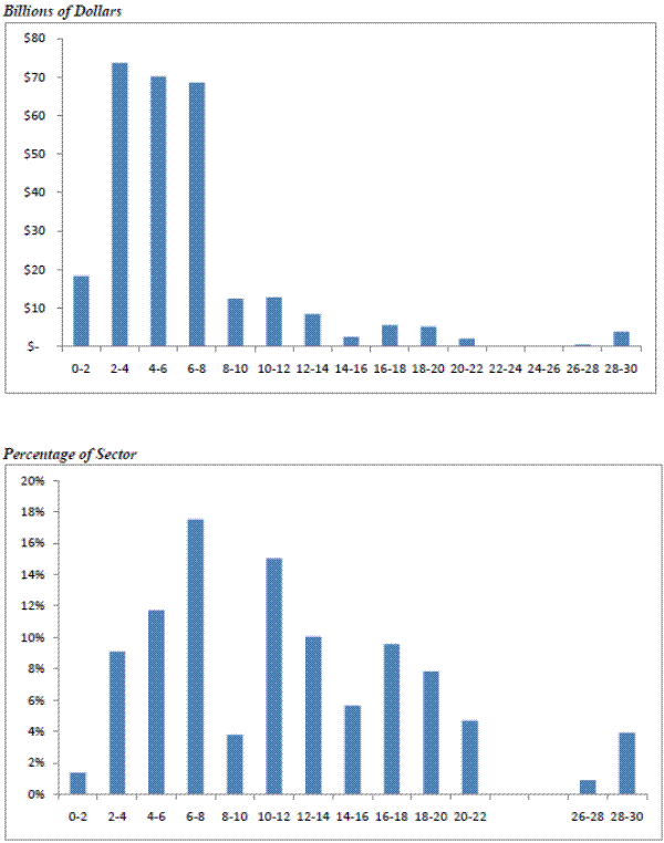 Figure 1 Data
Note: Denominator is par value of outstanding securities in each sector as of July 13, 2009. No securities were outstanding with remaining maturities between 22 and 26 years.
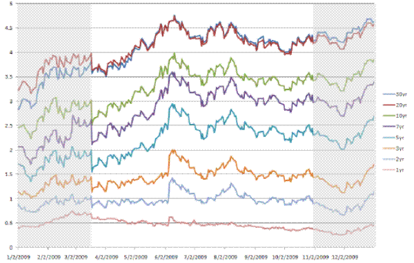
Notes: Yields are constant-maturity. Highlighted region shows the period (March 18 - October 30, 2009) during which the Treasury LSAP program was in effect.
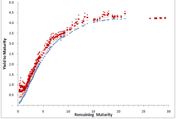
Notes: The dots are nominal yields on each of the 148 securities outstanding in our cross section as of October 30, 2009, based on the 148 securities in our cross section. The squares are the counterfactual yield point estimates on that day, using the same set of Treasury prices but with the estimated local-supply effects of LSAP purchases removed according to the coefficients in the last column of Table 5. The + and - signs are the 95 and 5 percent confidence bands around the counterfactual yields.
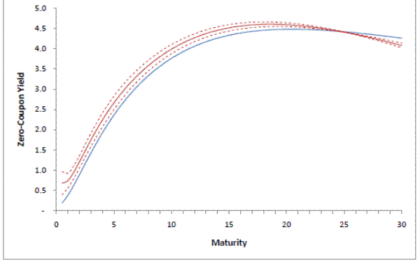
Notes: The thick solid line is the nominal yield curve as of October 30, 2009, based on the 148 securities in our cross section and constructed using the Svensson (1994) function. The thin solid line is the counterfactual yield curve on that day, using the same set of Treasury prices but with the estimated local-supply effects of LSAP purchases removed according to the coefficients in the last column of Table 5. Dotted lines show Svensson curves based on the 95 and 5 percent confidence bands around the counterfactual prices.
Table 1. Characteristics of Nominal Treasury LSAP Purchases
| Average of LSAP purchases | Average of all outstanding coupon securities | |
| Remaining maturity | 6.5 years | 5.7 years |
| Coupon | 3.7% | 3.8% |
| Yield | 2.4% | 1.9% |
| Time since issued | 4.0 years | 3.9 years |
| % On-the-run | 29.0% | 4.9% |
| % Notes | 79.5% | 82.8% |
Note: All figures are dollar-weighted averages over the period March 18 - October 29, 2009.
Table 2. Indicators of Liquidity in the Nominal Treasury Market
| Daily market volume | 10-year on-the-run premium | Fails to deliver | Average absolute fitting errors of Svensson curve | |
| March 25-July 6 2009 | $100 bil | 39 bp | $73 bil | 6.4 bp |
| July 7-October 29 2009 | $120 bil | 29 bp | $15 bil | 3.3 bp |
Notes: The table reports averages of daily values. Volume data come from Bloomberg, and fails-to-deliver data come from the FR 2004 reports. The on-the-run premium is the difference between the yield on the on-the-run 10-year note and 10-year value from a Svensson curve fit to off-the-run securities.
Table 3. LSAP Purchases as a Function of pre-LSAP Information
| Intercept | 0.051*** (0.015) |
| Remaining maturity | 0.015*** (0.003) |
| Remaining maturity squared | -0.0006*** (0.00009) |
| Svensson fitting error | 0.208*** (0.038) |
| % of issue held by Fed | -0.271*** (0.083) |
| On-the-run dummy | 0.091*** (0.024) |
| -0.044*** (0.014) | |
| # Obs | 148 |
| Adjusted R |
0.431 |
Notes: The dependent variable is the total amount of each security purchased under the LSAP program as a percentage of the total amount of that security outstanding. All independent variables are as of March 17, 2009. Standard errors in parentheses. *** indicates statistical significance at the 1 percent level.
Table 4. Stock Effects (IV)-Pooled
| Baseline | Controlling for initial prices | |
| Own Purchases (IV) | 2.17*** (0.43) | 0.61*** (0.21) |
| Purchases of near substitutes (IV) (maturity w/in 2 yrs of own) | 0.13** (0.07) | 0.07** (0.03) |
| Remaining maturity | -0.003** (0.001) | -0.0005 (0.0007) |
| Remaining maturity squared | 0.00003 (0.00004) | -0.00004 (0.00002) |
| Log initial price | - | 0.019*** (0.007) |
| Initial % fitting error | - | -0.58*** (0.07) |
| Intercept | 0.011*** (0.002) | -0.08** (0.03) |
| # Obs | 148 | 148 |
|---|---|---|
| Adj. R |
0.695 | 0.857 |
Notes: The dependent variable is the cumulative percentage holding return from March 17 to October 30, 2009. Regressions are 2SLS with March 17-dated variables used as instruments. All purchase variables are normalized by the total quantity of near substitutes outstanding. Asymptotic standard errors in parentheses. Asterisks indicate statistical significance at the 10 percent (*), 5 percent (**), and 1 percent (***) levels.
Table 5. Stock Effects (IV)-Subsamples
| Notes | Bonds | Near on-the-run | Far off-the-run | |||
| Own Purchases (IV) | 0.35 | 0.68*** | 0.38 | 0.66*** | -0.03 | 1.23*** |
| Own Purchases (IV) (Standard Error) | (0.32) | (0.24) | (0.31) | (0.21) | (0.34) | (0.34) |
| Purchases of near substitutes (IV) (maturity w/in 2 yrs of own) | 0.08** | 0.09* | 0.04 | 0.04 | 0.17*** | 0.11*** |
| Purchases of near substitutes (IV) (maturity w/in 2 yrs of own) (Standard Error) | (0.03) | (0.05) | (0.07) | (0.03) | (0.06) | (0.04) |
| Remaining maturity | -0.0006 | -0.0006 | -0.00007 | -0.00007 | -0.0022** | -0.0022** |
| Remaining maturity (Standard Error) | (0.0007) | (0.0007) | (0.0008) | (0.0008) | (0.0011) | (0.0011) |
| Remaining maturity squared | -0.00003 | -0.00003 | -0.00005* | -0.00005* | 0.00002 | 0.00002 |
| Remaining maturity squared (Standard Error) | (0.00002) | (0.00002) | (0.00003) | (0.00003) | (0.00004) | (0.00004) |
| Log initial price | 0.015 | 0.015 | 0.018*** | 0.018*** | 0.025** | 0.025** |
| Log initial price (Standard Error) | (0.0098) | (0.0098) | (0.007) | (0.007) | (0.0099) | (0.0099) |
| Initial % fitting error | -0.56*** | -0.56*** | -0.57*** | -0.57*** | -0.52*** | -0.52*** |
| Initial % fitting error (Standard Error) | (0.07) | (0.07) | (0.06) | (0.06) | (0.08) | (0.08) |
| Intercept | -0.06 | -0.06 | -0.07** | -0.07** | -0.11** | -0.11** |
| Intercept | (0.04) | (0.04) | (0.03) | (0.03) | (0.05) | (0.05) |
| # Obs | 148 | 148 | 148 | 148 | 148 | 148 |
|---|---|---|---|---|---|---|
| Adj. R |
0.903 | 0.903 | 0.904 | 0.904 | 0.914 | 0.914 |
Notes: The dependent variable is the cumulative percentage holding return from March 17 to October 30, 2009. Regressions are 2SLS with March 17-dated variables used as instruments. All purchase variables are normalized by the total quantity of near substitutes outstanding. Asymptotic standard errors in parentheses. Asterisks indicate statistical significance at the 10 percent (*), 5 percent (**), and 1 percent (***) levels.
Table 6. Flow Effects on Day of Purchase (eligible securities)
| Own Purchases | 0.276*** | -0.106 |
| Own Purchases (Standard Error) | (0.053) | (0.098) |
| Purchases of: Near substitutes (maturity w/in 2 yrs of own) | 0.240*** | -0.124*** |
| Purchases of: Near substitutes (maturity w/in 2 yrs of own) (Standard Error) | (0.048) | (0.044) |
| Purchases of: Mid-substitutes (maturity 2 to 6 years away) | 0.170*** | -0.050* |
| Purchases of: Mid-substitutes (maturity 2 to 6 years away) (Standard Error) | (0.045) | (0.026) |
| # Obs. | 923 | 145 |
| # CUSIPS | 146 | 23 |
| Adj. R |
0.976 | 0.985 |
Notes: The dependent variable is the daily percentage price change in each outstanding CUSIP. Only securities that were eligible to be purchased in a given operation are included. Fixed effects and daily time dummies not shown. Standard errors in parentheses. Asterisks indicate statistical significance at the 10 percent (*), 5 percent (**), and 1 percent (***) levels.
Table 7. Flow Effects on Day of Purchase, by Subsamples (eligible securities with remaining maturity ![]() 15 years)
15 years)
| Mar 25 - Jul 6 | Jul 7 - Oct. 29 | Notes | Bonds | Near on-the-run | Far off-the-run | |
| Own Purchases | 0.3442*** | 0.2975*** | 0.2669*** | 0.2498*** | 0.2318** | 0.2488*** |
| Own Purchases (Standard Error) | (0.094) | (0.089) | (0.068) | (0.090) | (0.107) | (0.065) |
| Purchases of: Near substitutes (maturity w/in 2 yrs of own) | 0.2863*** | 0.3038*** | 0.2503*** | 0.1694** | 0.2435** | 0.1584*** |
| Purchases of: Near substitutes (maturity w/in 2 yrs of own) (Standard Error) | (0.086) | (0.083) | (0.062) | (0.083) | (0.105) | (0.057) |
| Purchases of: Mid-substitutes (maturity 2 to 6 years away) | 0.1989*** | 0.2037** | 0.2088** | 0.0929 | 0.2501*** | 0.0744 |
| Purchases of: Mid-substitutes (maturity 2 to 6 years away) (Standard Error) | (0.082) | (0.073) | (0.055) | (0.080) | (0.092) | (0.055) |
| # Obs. | 563 | 360 | 769 | 154 | 249 | 674 |
| # CUSIPS | 131 | 121 | 123 | 23 | 53 | 114 |
| Adj. R |
0.974 | 0.975 | 0.976 | 0.986 | 0.986 | 0.977 |
Notes: The dependent variable is the daily percentage price change in each outstanding CUSIP. Only days when LSAP purchases occurred are included. Fixed effects and daily time dummies not shown. Standard errors in parentheses. Asterisks indicate statistical significance at the 10 percent (*), 5 percent (**), and 1 percent (***) levels.
Table 8. Flow Effects on Day of Purchase (Ineligible securities)
| Purchases of: Near substitutes (maturity w/in 2 yrs of own) | 0.0665*** | -0.0268 |
| Purchases of: Near substitutes (maturity w/in 2 yrs of own) (Standard Error) | (0.018) | (0.053) |
| Purchases of: Mid-substitutes (maturity 2 to 6 years away) | 0.0047 | -0.007 |
| Purchases of: Mid-substitutes (maturity 2 to 6 years away) (Standard Error) | (0.0099) | (0.021) |
| Purchases of: Far substitutes (maturity 6 to 14 years away) | -0.0238** | 0.0021 |
| Purchases of: Far substitutes (maturity 6 to 14 years away) (Standard Error) | (0.008) | (0.003) |
| # Obs. | 8008 | 1104 |
| # CUSIPS | 181 | 23 |
| Adj. R |
0.52 | 0.96 |
Notes: The dependent variable is the daily percentage price change in each outstanding CUSIP. Only securities that were not eligible to be purchased on days when operations occurred are included. Fixed effects and daily time dummies not shown. Standard errors in parentheses. Asterisks indicate statistical significance at the 10 percent (*), 5 percent (**), and 1 percent (***) levels.
Table 9. Flow Effects on Day of Purchase, by Sub-Period (Ineligible securities, remaining maturity ![]() 15 years)
15 years)
| Mar 25 - Jul 6 | Jul 7 - Oct. 29 | |
| Purchases of: Near substitutes (maturity w/in 2 yrs of own) | -0.127*** | 0.384*** |
| Purchases of: Near substitutes (maturity w/in 2 yrs of own) (Standard Error) | (0.025) | (0.031) |
| Purchases of: Mid-substitutes (maturity 2 to 6 years away) | -0.143*** | 0.202*** |
| Purchases of: Mid-substitutes (maturity 2 to 6 years away) (Standard Error) | (0.015) | (0.017) |
| Purchases of: Far substitutes (maturity 6 to 14 years away) | -0.153*** | 0.093*** |
| Purchases of: Far substitutes (maturity 6 to 14 years away) (Standard Error) | (0.014) | (0.011) |
| # Obs. | 4529 | 3479 |
| # CUSIPS | 167 | 172 |
| Adj. R |
0.51 | 0.57 |
Notes: The dependent variable is the daily percentage price change in each outstanding CUSIP. Only days when LSAP purchases occurred are included. Fixed effects and daily time dummies not shown. Standard errors in parentheses. Asterisks indicate statistical significance at the 10 percent (*), 5 percent (**), and 1 percent (***) levels.
Table 10. Flow Effects on Day of Purchase, by Security Type and Sub-Period (remaining maturity ![]() 15 years)
15 years)
Notes
| Eligible Securities Mar 25 - Jul 6 | Eligible Securities Jul 7 - Oct. 29 | Ineligible Securities Mar 25 - Jul 6 | Ineligible Securities Jul 7 - Oct. 29 | |
| Own Purchases | 0.445*** | 0.245** | - | - |
| Own Purchases | (0.147) | (0.122) (Standard Error) | - | - |
| Purchases of: Near substitutes (maturity w/in 2 yrs of own) | 0.396*** | 0.314*** | -0.213*** | 0.486*** |
| Purchases of: Near substitutes (maturity w/in 2 yrs of own) (Standard Error) | (0.148) | (0.107) | (0.041) | (0.049) |
| Purchases of: Mid-substitutes (maturity 2 to 6 years away) | 0.346*** | 0.260*** | -0.244*** | 0.266*** |
| Purchases of: Mid-substitutes (maturity 2 to 6 years away) (Standard Error) | (0.144) | (0.086) | (0.037) | (0.038) |
| Purchases of: Far substitutes (maturity 6 to 14 years away) | - | - | -0.061*** | 0.063*** |
| Purchases of: Far substitutes (maturity 6 to 14 years away) (Standard Error) | - | - | (0.040) | (0.039) |
| # Obs. | 442 | 327 | 3891 | 2960 |
| # CUSIPS | 108 | 111 | 144 | 149 |
| Adj. R |
0.979 | 0.972 | 0.477 | 0.548 |
Bonds
| Eligible Securities Mar 25 - Jul 6 | Eligible Securities Jul 7 - Oct. 29 | Ineligible Securities Mar 25 - Jul 6 | Ineligible Securities Jul 7 - Oct. 29 | |
| Own Purchases | 0.381*** | 0.108 | - | - |
| Own Purchases | (0.159) | (0.129) (Standard Error) | - | - |
| Purchases of: Near substitutes (maturity w/in 2 yrs of own) | 0.270*** | 0.011 | -0.208*** | 0.084* |
| Purchases of: Near substitutes (maturity w/in 2 yrs of own) (Standard Error) | (0.109) | (0.134) | (0.049) | (0.046) |
| Purchases of: Mid-substitutes (maturity 2 to 6 years away) | 0.178* | -0.161 | -0.077*** | 0.074*** |
| Purchases of: Mid-substitutes (maturity 2 to 6 years away) (Standard Error) | (0.104) | (0.134) | (0.019) | (0.020) |
| Purchases of: Far substitutes (maturity 6 to 14 years away) | - | -- | -0.077*** | 0.041*** |
| Purchases of: Far substitutes (maturity 6 to 14 years away) (Standard Error) | - | -- | (0.014) | (0.012) |
| # Obs. | 121 | 33 | 638 | 519 |
| # CUSIPS | 23 | 10 | 23 | 23 |
| Adj. R |
0.978 | 0.994 | 0.946 | 0.939 |
Notes: The dependent variable is the daily percentage price change in each outstanding CUSIP. Only days when LSAP purchases occurred are included. Fixed effects and daily time dummies not shown. Standard errors in parentheses. Asterisks indicate statistical significance at the 10 percent (*), 5 percent (**), and 1 percent (***) levels.
Table 11. Flow Effects on Day after Purchase, by Security Type and Sub-Period (remaining maturity ![]() 15 years)
15 years)
Notes
| Eligible Securities Mar 25 - Jul 6 | Eligible Securities Jul 7 - Oct. 29 | Ineligible Securities Mar 25 - Jul 6 | Ineligible Securities Jul 7 - Oct. 29 | |
| Own Purchases | -0.379*** | -0.145 | - | - |
| Own Purchases (Standard Error) | (0.143) | (0.116) | - | - |
| Purchases of: Near substitutes (maturity w/in 2 yrs of own) | -0.478*** | -0.152 | -0.464*** | -0.135*** |
| Purchases of: Near substitutes (maturity w/in 2 yrs of own) (Standard Error) | (0.145) | (0.108) | (0.039) | (0.049) |
| Purchases of: Mid-substitutes (maturity 2 to 6 years away) | -0.620*** | -0.106 | -0.436*** | -0.009 |
| Purchases of: Mid-substitutes (maturity 2 to 6 years away) (Standard Error) | (0.139) | (0.087) | (0.035) | (0.039) |
| Purchases of: Far substitutes (maturity 6 to 14 years away) | - | - | -3.08*** | 0.134*** |
| Purchases of: Far substitutes (maturity 6 to 14 years away) (Standard Error) | - | - | (0.039) | (0.038) |
| # Obs. | 442 | 327 | 3886 | 2957 |
| # CUSIPS | 108 | 111 | 144 | 149 |
| Adj. R |
0.986 | 0.974 | 0.573 | 0.507 |
Bonds
| Eligible Securities Mar 25 - Jul 6 | Eligible Securities Jul 7 - Oct. 29 | Ineligible Securities Mar 25 - Jul 6 | Ineligible Securities Jul 7 - Oct. 29 | |
| Own Purchases | 0.377*** | 0.58*** | - | - |
| Own Purchases | (0.145) | (0.117) (Standard Error) | - | - |
| Purchases of: Near substitutes (maturity w/in 2 yrs of own) | 0.157 | 0.556*** | -0.047 | 0.086* |
| Purchases of: Near substitutes (maturity w/in 2 yrs of own) (Standard Error) | (0.098) | (0.119) | (0.046) | (0.047) |
| Purchases of: Mid-substitutes (maturity 2 to 6 years away) | 0.111 | 0.472*** | -0.057*** | -0.046*** |
| Purchases of: Mid-substitutes (maturity 2 to 6 years away) (Standard Error) | (0.082) | (0.125) | (0.018) | (0.020) |
| Purchases of: Far substitutes (maturity 6 to 14 years away) | - | - | -0.049*** | 0.015*** |
| Purchases of: Far substitutes (maturity 6 to 14 years away) (Standard Error) | - | - | (0.014) | (0.013) |
| # Obs. | 121 | 33 | 638 | 519 |
| # CUSIPS | 23 | 10 | 23 | 23 |
| Adj. R |
0.99 | 0.99 | 0.94 | 0.93 |
Notes: The dependent variable is the daily percentage price change in each outstanding CUSIP. Only days when LSAP purchases occurred are included. Fixed effects and daily time dummies not shown. Standard errors in parentheses. Asterisks indicate statistical significance at the 10 percent (*), 5 percent (**), and 1 percent (***) levels.
Table 12. Flow Effects on Day of Purchase, All Securities Clustered Standard Errors
| Eligible Securities |
Eligible Securities |
Ineligible Securities |
Ineligible Securities |
|
| Own Purchases | 0.2763*** | -0.1063 | - | - |
| Own Purchases (Standard Error) | (0.044) | (0.089) | - | - |
| Purchases of: Near substitutes (maturity w/in 2 yrs of own) | 0.2403*** | -0.1238*** | 0.0665*** | -0.0268 |
| Purchases of: Near substitutes (maturity w/in 2 yrs of own) (Standard Error) | (0.038) | (0.029) | (0.029) | (0.017) |
| Purchases of: Mid-substitutes (maturity 2 to 6 years away) | 0.1700*** | -0.0501** | 0.0047 | -0.007 |
| Purchases of: Mid-substitutes (maturity 2 to 6 years away) (Standard Error) | (0.053) | (0.014) | (0.016) | (0.037) |
| Purchases of: Far substitutes (maturity 6 to 14 years away) | - | - | -0.0238** | 0.0021 |
| Purchases of: Far substitutes (maturity 6 to 14 years away) (Standard Error) | - | - | (0.009) | (0.003) |
| # Obs. | 923 | 145 | 8008 | 1104 |
| # CUSIPS | 146 | 23 | 181 | 23 |
| Adj. R |
0.976 | 0.985 | 0.519 | 0.968 |
Notes: The dependent variable is the daily percentage price change in each outstanding CUSIP. Only days when LSAP purchases occurred are included. Fixed effects and daily time dummies not shown. Standard errors in parentheses. Asterisks indicate statistical significance at the 10 percent (*), 5 percent (**), and 1 percent (***) levels.
Table 13. Flow Effects on Day of Purchase, by Security Type and Vintage (Eligible securities with remaining maturity ![]() 15 years) Clustered Standard
Errors
15 years) Clustered Standard
Errors
| Bonds | Notes | Near on-the-run | Far off-the-run | |
| Own Purchases | 0.2498** | 0.2669*** | 0.2318** | 0.2488*** |
| Own Purchases (Standard Error) | (0.06) | (0.058) | (0.098) | (0.051) |
| Purchases of: Near substitutes (maturity w/in 2 yrs of own) | 0.1694** | 0.2503*** | 0.2435** | 0.1584*** |
| Purchases of: Near substitutes (maturity w/in 2 yrs of own) (Standard Error) | (0.03) | (0.051) | (0.073) | (0.029) |
| Purchases of: Mid-substitutes (maturity 2 to 6 years away) | 0.0929 | 0.2088** | 0.2501*** | 0.0744 |
| Purchases of: Mid-substitutes (maturity 2 to 6 years away) (Standard Error) | (0.035) | (0.059) | (0.059) | (0.026) |
| # Obs. | 154 | 769 | 249 | 674 |
| # CUSIPS | 23 | 123 | 53 | 114 |
| Adj. R |
0.986 | 0.976 | 0.986 | 0.977 |
Notes: The dependent variable is the daily percentage price change in each outstanding CUSIP. Only days when LSAP purchases occurred are included. Fixed effects and daily time dummies not shown. Standard errors in parentheses. Asterisks indicate statistical significance at the 10 percent (*), 5 percent (**), and 1 percent (***) levels.
Acknowledgements
For helpful discussions and comments we thank other members of the Staff at the Federal Reserve Board and the Federal Reserve Bank of New York, as well as Greg Duffee, Michael Fleming, James Hamilton, Chris Lamereaux, Monika Piazzesi, Tsutomu Watanabe, Min Wei, Jonathan Wright, Dave Zervos, and seminar participants at the Bank of England, the Banco de España, Cal State Fullerton, the Federal Reserve System Real-Time Policy Conference, the Federal Reserve Bank of San Francisco conference on Monetary Policy at the Zero Lower Bound, and the Federal Reserve Bank of St. Louis conference on Quantitative Easing. Shenje Hshieh, Alex Jutca, and Elizabeth Lewis provided excellent research assistance. Remaining errors are ours alone. The views expressed here do not reflect official positions of the Federal Reserve.
References
Amihud, Y. and Mendelson, H., 1991. Liquidity, Maturity, and the Yields on U.S. Treasury Securities. Journal of Finance 46, 1411-1425.
Andres, J.; Lopez-Salido, J. D.; and Nelson, E., 2004. Tobin's Imperfect Asset Substitution in Optimizing General Equilibrium. Journal of Money, Credit, and Banking 36, 665-690.
Bernanke, B. S.; Reinhart, V. R.; and Sack, B. P., 2004. Monetary Policy Alternatives at the Zero Bound: An Empirical Assessment. Brookings Papers on Economic Activity 2, 1-78.
Brandt, M.W. and Kavajecz K. A., 2004. Price Discovery in the U.S. Treasury Market: The Impact of Orderflow and Liquidity on the Yield Curve. Journal of Finance 59, 2623-2654.
Cochrane, J. H., 2008. Comments on `Bonds Supply and Excess Bond Returns' by Robin Greenwood and Dimitri Vayanos. May 12.
Cox, J. C.; Ingersoll, J. E.; and Ross, S. A, 1985. A Theory of the Term Structure of Interest Rates. Econometrica 53, 385-407.
Culbertson, J. M., 1957. The Term Structure of Interest Rates. Quarterly Journal of Economics 71, 485-517.
Engen, E. and Hubbard, R. G., 2005. Federal Government Debt and Interest Rates. In Gertler and Rogoff (eds.), NBER Macroeconomics Annual 2004. Cambridge, MA: The MIT Press.
Gabaix, X.; Krishnamurthy, A.; and Vigneron, O., 2007. Limits of Arbitrage: Theory and Evidence from the Mortgage-Backed Securities Market. Journal of Finance 62, 557-595.
Gagnon, J.; Raskin, M.; Remache, J,; and Sack, B., 2010. Large-Scale Asset Purchases by the Federal Reserve: Did They Work? FRB New York Staff Report 441.
Garleanu, N.; Pedersen, L. H.; and Poteshman, A. M., 2009. Demand-Based Option Pricing. Review of Financial Studies 22, 4259-4299.
Greenwood, R., 2005. Short- and Long-Term Demand Curves for Stocks: Theory and Evidence on the Dynamics of Arbitrage. Journal of Financial Economics 75, 607-649.
Greenwood, R. and Vayanos, D., 2010a. Price Pressure in the Government Bond Market. American Economic Review 100, 585-590.
Greenwood, R. and Vayanos, D., 2010b, Bond Supply and Excess Bond Returns. NBER Working Paper 13806.
Gromb, D. and Vayanos, D., 2010. Limits to Arbitrage: The State of the Theory. Working paper, April.
Gurkyanak, R.; Sack, B.; and Wright, J., 2007. The U.S. Treasury Yield Curve: 1961 to the Present. Journal of Monetary Economics 54, 2291-2304.
Gurkyanak, R. and Wright, J., 2010. Macroeconomics and the Term Structure. Mimeo, April.
Hamilton, J. and Wu, J., 2010. The Effectiveness of Alternative Monetary Policy Tools in a Zero Lower Bound Environment. Mimeo, August.
Han, B.; Longstaff, F. A.; and Merrill, C., 2007. The U.S. Treasury Buyback Auctions: The Cost of Retiring Illiquid Bonds. Journal of Finance 62, 2673-2693.
Holland, T. E., 1969. 'Operation Twist' and the Movement of Interest Rates and Related Economic Time Series. International Economic Review 10, 260-265.
Hu, X.; Pan, J.; and Jiang, W., 2010. Noise as Information for Illiquidity. NBER working paper 16468.
Krishnamurthy, A., 2002. The Bond/Old-Bond Spread. Journal of Financial Economics 66, 463-506.
Krishnamurthy, A. and Vissing-Jorgensen, A., 2007. The Demand for Treasury Debt. NBER Working Paper 12881.
Kaminska, I.; Vayanos, V,; and Zinna, G., 2011. Preferred-Habitat Investors and the US Term Structure of Real Rates. Bank of England working paper 435, July.
Kuttner, K., 2006. Can Central Banks Target Bond Prices? NBER Working Paper 12454.
Longstaff, F. A., 2004. The Flight-to-Liquidity Premium in U.S. Treasury Bond Prices. Journal of Business 77, 511-526.
Lou, D.; Yan, H.; and Zhang, J., 2010. Anticipated and Repeated Shocks in Liquid Markets. Working paper.
Meaning, J. and Zhu, F., 2011. The Impact of Recent Central Bank Purchase Programmes. BIS Quarterly Review (December),73-83.
Modigliani, F. and Sutch, R., 1966. Innovations in Interest Rate Policy. American Economic Review 56, 178-197.
Musto, D.; Nini, G.; Schwarz, K., 2011. Notes on Bonds: Liquidity at All Costs in the Great Recession. Working paper, April 27.
Neely, C. J., 2010. The Large Scale Asset Purchases Had Large International Effects. FRB St. Louis Working Paper 2010-018A.
Ross, M., 1966. `Operation Twist': A Mistaken Policy? Journal of Political Economy 74, 195-199.
Svensson, L. E. O., 1994. Estimating and Interpreting Forward Rates: Sweden 1992-4, NBER Working Paper 4871.
Swanson, E. T., 2011. Let's Twist Again: A High-Frequency Event-Study Analysis of Operation Twist and Its Implications for QE2. Federal Reserve Bank of San Francisco working paper.
Thornton D. L., 2009. The Effect of the Fed's Purchase of Long-Term Treasuries on the Yield Curve, FRB St. Louis Economic Synopses 25.
Vayanos, D. and Vila, J-L., 2009. A Preferred-Habitat Model of the Term Structure of Interest Rates. NBER Working Paper 15487.