
The Federal Reserve's Balance Sheet and Overnight Interest Rates*
Keywords: Reserve balances, federal funds rate, balance sheet, large-scale asset purchases, interest rate on excess reserves, exit strategy
Abstract:
This paper provides a comprehensive study of the interplay between the Federal Reserve's balance sheet and overnight interest rates. We model both the supply of and the demand for excess reserves, treating assets of the Federal Reserve as policy tools, and estimate the effects of conventional and unconventional monetary policy on overnight funding rates. We find that, in the current environment with quite elevated levels of reserves, the effect of further monetary policy accommodation on overnight interest rates is limited. Further, assuming a path for removing monetary policy accommodation that is consistent with the FOMC's exit principles, we project that the federal funds rate increases to 70 basis points, settling in a corridor bracketed by the discount rate and the interest rate on excess reserves, as excess reserves of depository institutions decline to near zero.
1 Introduction
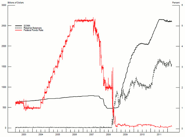
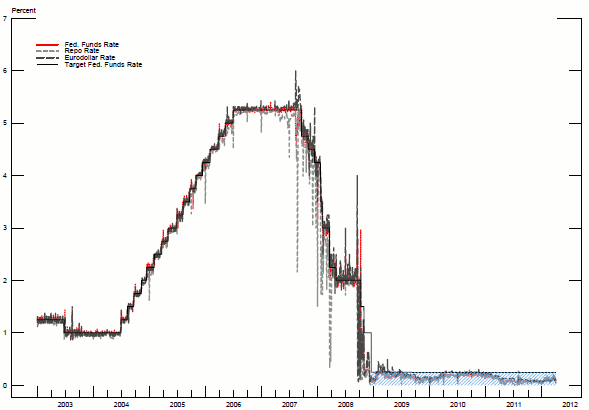
In response to the financial crisis of 2008, the Federal Reserve adopted a variety of unconventional monetary policy measures.4 The use of these measures led to an unprecedented change in the size and composition of the Federal Reserve's balance sheet that affected short-term interest rates.5 Initially, the Federal Reserve implemented various liquidity facilities to promote the functioning of financial markets. The associated increase on the asset side of the Federal Reserve's balance sheet was matched by a comparable increase in reserve balances on the liability side of the balance sheet.6 As the crisis went on and various liquidity facilities wound down, the Federal Reserve began its large-scale asset purchases. Reducing the amount of privately-held securities was intended to reduce longer-term interest rates. Besides putting downward pressure on longer-term interest rates, the unconventional policy actions resulted in an unprecedented increase in reserve balances of depository institutions (DIs). Over this period, as reserve balances increased, short-term interest rates experienced an unprecedented deline (Figure 1). Indeed, the federal funds rate and other short-term interest rates reached their zero lower bound and have remained there since.7
The purpose of this paper is to model the interplay between the Federal Reserve's balance sheet and overnight interest rates, while allowing for interdependencies among these rates. This framework is used to assess the effect of both conventional and unconventional monetary policy changes on overnight interest rates. In particular, we study both the impact of further policy accommodation by the Federal Reserve and the removal of the monetary policy accommodation currently in place. Our exit strategy simulation is based on the exit principles specified in the June 2011 minutes of the Federal Open Market Committee (FOMC), FOMC (2011b).
Our results suggest that, in the current environment, where the level of excess reserve balances is quite elevated by historical standards, the demand curve for these balances is extremely flat: Further monetary policy accommodation therefore puts only limited downward pressure on overnight interest rates. Furthermore, under certain assumptions about the path for the removal of monetary policy accommodation that is consistent with the June 2011 FOMC exit principles, our projections suggest that the accommodative stance of monetary policy in place since 2008 is effectively reversed and excess reserves return to a normal level by historical standards. Under our assumptions, excess reserves of DIs decline to a level close to that observed prior to the crisis, which results in an increase in the federal funds rate to 70 basis points by 2016, a level that is in the middle of the corridor bracketed by the discount rate and the interest rate on excess reserves (IOER rate).
Our framework differentiates the demand for reserves from the supply of reserves. To model the supply of reserve balances, we treat the assets of the Federal Reserve as policy variables and endogenize its liabilities. Specifically, we model required reserve balances held by DIs as a function of reservable deposits held at banks.8Excess reserves respond to ensure that total assets of the Federal Reserve equal total liabilities plus capital. The demand for reserve balances is modeled as a non-linear, simultaneous system of equations determining the federal funds rate, the Treasury general collateral (GC) repo rate, and the Eurodollar rate.
Our work contributes to the literature in several ways. First, this paper extends previous work on the "liquidity effect"--the response of short-term interest rates to a change in the amount of reserve balances--as documented by Hamilton (1996) and Hamilton (1997).9 Specifically, previous empirical work on the liquidity effect, except for Bech et al. (2012), quantifies the effect of monetary policy changes with no allowance for interdependencies among short-term interest rates. In contrast, we accommodate linkages among banks' various short-term funding options with the associated implications for overnight rates. Specifically, in our framework, a change in the federal funds rate simultaneously affects the repo rate and the Eurodollar rate; these changes then feed back to the federal funds rate. Second, we use the full-information maximum likelihood method for parameter estimation in order to account for the simultaneous determination of reserves and the federal funds rate. Previous work uses limited information estimation methods to avoid simultaneity biases. Nevertheless, this approach is not suited for our work because it treats reserves as endogenous for parameter estimation but exogenous for policy analysis. Third, previous studies generally focus on the short-term dynamics of interest rates to temporary changes in reserve balances.10 Information on short-run dynamics, however, is not sufficient to study the effects of unconventional monetary policy and the removal of such policy. Our framework encompasses both short-run dynamics and steady states as well as their responses to temporary and permanent changes in policy actions. Fourth, the prior literature is mostly concerned with interest rate responses to changes in reserve balances. In contrast, we examine the relation between the levels of overnight interest rates and reserve balances, which allows us to answer important policy questions, such as the determination of the amount of reserve balances consistent with a certain level for the federal funds rate. Finally, all of these extensions can be used to assess the effects of monetary policy actions at the zero lower bound. In particular, we investigate the implications of further monetary policy accommodation and of an exit strategy, that is consistent with the June 2011 FOMC exit principles, on short-term interest rates.
The remainder of the paper proceeds as follows: Section 2 describes our empirical framework, designed to capture the interplay between the evolution of the Federal Reserve's balance sheet and overnight interest rates. Section 3 presents the estimation results. Section 4 shows projections of the effects of conventional and unconventional monetary policy on overnight interest rates. Section 5 concludes.
2.1 Supply of Reserve Balances
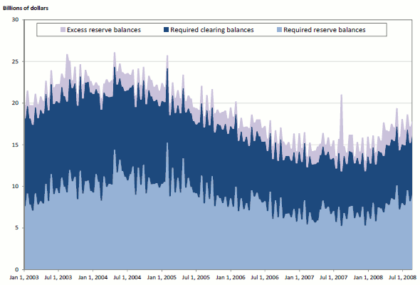
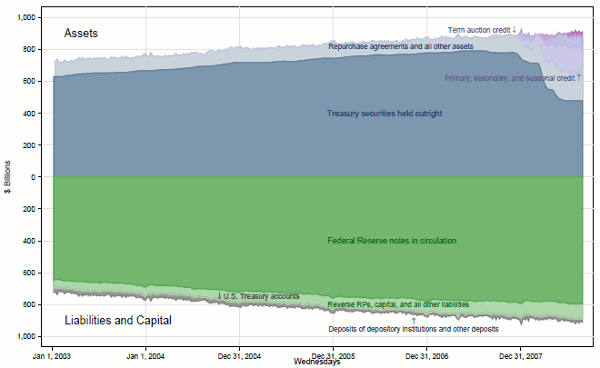
Prior to the financial crisis, temporary open market operations (e.g., repurchase agreements) were the primary means of monetary policy by which aggregate reserve balances were altered in order to attain the target federal funds rate set by the FOMC.11 These operations were so finely tuned that reserve balances of DIs rarely exceeded $25 billion (Figure 2), of which balances held in excess of balance requirements represented only a tiny fraction.12 Federal Reserve notes (currency) in circulation constituted the largest liability and were collateralized by holdings of U.S. Treasury securities, the largest asset of the Federal Reserve (Figure 3).13
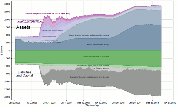
The initial response of the Federal Reserve to the financial crisis involved implementing various liquidity facilities to support the functioning of funding markets. As shown in Figure 4, the expansion of these facilities was initially sterilized through sales and redemptions of U.S. Treasury securities in an attempt to be " reserve-neutral" (see Open Market Operations Report (2008)). As the crisis continued, however, the Federal Reserve abandoned its sterilization efforts, while continuing to inject ample liquidity into the market. Repurchase agreements were brought to zero and replaced with outright acquisitions of substantial amounts of U.S. Treasury securities, Agency debt securities, and Agency mortgage-backed securities (MBS). These purchases increased deposits of DIs, which became the largest liability; most of these deposits constitute excess reserves. In the end, the size of the balance sheet (total assets) increased from $877 billion by the end of August 2007 to about $2.9 trillion by the end of April 2012.
For modeling purposes, we treat all securities holdings of the Federal Reserve as a single asset. This treatment assumes that U.S. Treasury securities, Agency MBS, and Agency debt securities are perfect substitutes and thus can be combined into a single aggregate that we denote by ![]() . We retain explicitly repurchase agreements (
. We retain explicitly repurchase agreements (![]() , even though they are currently zero, because
a resumption of normal market functioning may renew the interest in temporary open market operations. Foreign exchange swaps and loans extended through either the discount window or the liquidity facilities are combined into other assets (
, even though they are currently zero, because
a resumption of normal market functioning may renew the interest in temporary open market operations. Foreign exchange swaps and loans extended through either the discount window or the liquidity facilities are combined into other assets (![]() ). In terms of liabilities, we disaggregate reserves into excess reserves (
). In terms of liabilities, we disaggregate reserves into excess reserves (![]() and required reserves (
and required reserves (![]() ); we account for currency in circulation (
); we account for currency in circulation (![]() ) separately because of its large magnitude. All other liabilities
(e.g., the U.S. Treasury's General Account, reverse repurchase agreements, and term deposits) as well as capital are combined into other liabilities (
) separately because of its large magnitude. All other liabilities
(e.g., the U.S. Treasury's General Account, reverse repurchase agreements, and term deposits) as well as capital are combined into other liabilities (![]() ). The simplified balance-sheet identity
is
). The simplified balance-sheet identity
is
We assume that
We model ![]() as a fraction
as a fraction ![]() of " reservable" deposits
of " reservable" deposits ![]() held at DIs:14
held at DIs:14
where
where
To determine the supply of excess reserves, we substitute equation (3) into equation (2) and solve for ![]() in equation (1) to
obtain
in equation (1) to
obtain
 |
(4) |
which ensures that the Federal Reserve's total assets equal total liabilities plus capital. Note that
 |
(5) |
In other words, an increase in the federal funds rate raises the supply of excess reserves, all else constant. Intuitively, holding constant the size of the Federal Reserve's balance sheet and total reserves, a higher federal funds rate reduces transaction deposits, which lowers required reserves. Lower required reserves, with constant total reserves, means more excess reserves.
2.2 Demand for Reserve Balances
We assume that the (inverse) demand for excess reserve balances can be expressed as:
where
As shown in Figure 5, the federal funds, the repo, and the Eurodollar rates co-move around the intended target rate set by the FOMC.17 These co-movements stem from the overlap of participants in various funding markets that generally leads to active arbitrage across these markets. Indeed, as noted in the top row of Table 1, DIs borrow in all three markets. DIs generally rely on federal funds and Eurodollars as sources of borrowing to meet general short-term funding needs. In addition, since the advent of payment of interest on reserves, DIs have also borrowed in these markets to arbitrage the market rates against the higher IOER rate. Institutions borrowing in the repo market--which include DIs, broker dealers, and others--typically finance the specific assets pledged as collateral in the trade. On the lending side of the markets, as shown in the bottom row of the table, there is more segmentation in participation across the markets. Depository institutions, broker dealers, and government-sponsored enterprises (GSEs) are the lenders in the federal funds market. Even though GSEs could lend Eurodollars as well, they tend, in practice, to be less active in this market. They are, however, active participants in the repo market. Money market mutual funds are active lenders in the Eurodollar market and in the repo market.
Given these interdependencies, we endogenize both ![]() and
and
![]() as
as
| (7) | ||
| (8) |
Taken together, equations (6)-(8) extend the literature on the liquidity effect by recognizing interdependencies among wholesale funding markets and by including the IOER rate as an additional tool of monetary policy.
2.3 Transmission Channels
Changes in ![]() affect the federal funds rate through several channels. First, a reduction in
affect the federal funds rate through several channels. First, a reduction in ![]() reduces reserve balances, as DIs' deposits at the Federal Reserve are debited when DIs purchase the securities.18 These sales reduce excess
reserves, which increases the federal funds rate:
reduces reserve balances, as DIs' deposits at the Federal Reserve are debited when DIs purchase the securities.18 These sales reduce excess
reserves, which increases the federal funds rate:
Second, this increase in the federal funds rate raises the borrowing cost in all other funding markets, which then feeds back to the federal funds rate:
 |
Finally, these increases in ![]() raise the opportunity cost of holding reservable deposits and reduce
raise the opportunity cost of holding reservable deposits and reduce ![]() This reduction lowers reserve requirements, raises excess reserves, and lowers the federal funds rate:
This reduction lowers reserve requirements, raises excess reserves, and lowers the federal funds rate:
Thus, the direction of the response of ![]() to a change in
to a change in ![]() is not known in
advance. We resolve this ambiguity empirically by specifying and estimating an econometric model.
is not known in
advance. We resolve this ambiguity empirically by specifying and estimating an econometric model.
2.4 Model Specification
We postulate the following econometric model:
This model has three interesting properties. First, it allows for delayed responses to changes in market conditions. Second, modeling the logarithm of interest rates allows to capture non-linearities. Finally, it includes the interest rate on excess reserves. This inclusion raises estimation challenges because this rate was "zero" prior to October 2008 and exhibited wide swings right after its introduction, before stabilizing at 25 basis points. To control for the "novelty" of this rate during its initial phase, we include a dummy variable in equation (9), not shown, with a value of 1 from October 2008 to December 2008 and zero otherwise.19
Given the model, the response of the federal funds rate to a change in ![]() is
is
![\displaystyle \frac{\partial i^{fed}}{\partial S}=i^{fed}\cdot \left[ \frac{\ov... ...da }_{1}\widetilde{\phi }_{2}\widetilde{\alpha }_{4}}}}% \right] \lesseqqgtr 0,](img50.gif) |
(15) |
where tildes denote long-run coefficients (e.g.,
3.1 Sample Selection
The data consist of daily observations (business days) from January 10, 2003 to March 30, 2012. We use this period for estimation because alternative periods, as discussed below, are not helpful in assessing the exit strategy principles:
- Alternative 1: Use exclusively the pre-crisis period because subsequent observations are from a distorted sample. This alternative, however, cannot possibly recognize the role of the interest rate on excess reserves, which is problematic because the principles rely on this tool.
- Alternative 2: Use exclusively the post-crisis sample because the crisis represents a break with the past. This alternative is problematic because the variability of interest rates in this period is virtually absent, and, hence, the rates are not statistically reliable for assessing the principles.
- Alternative 3: Use the pre-crisis sample to estimate a set of parameters and the post-crisis sample to estimate another set of parameters.20 This approach assumes that, as excess reserves are drained to their pre-crisis level, the economy switches automatically from the post-crisis parameter values to the pre-crisis parameter values. But, because the pre-crisis parameters are estimated before the introduction of interest payments on excess reserves and the Term Deposit Facility, these estimates are not applicable to the exit period.
3.2 Estimation Results
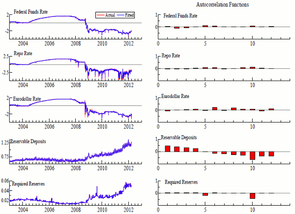
We use the full-information maximum likelihood (FIML) method to estimate the parameters of equations (9)-(14).21 In terms of coefficient estimates, the results in Table 2 confirm the inverse, and statistically significant, relation between excess reserves and the federal funds rate. The results also confirm the interdependencies among overnight interest rates: the coefficients are positive and highly significant. As shown in Figure 6, the model has a good fit with a large degree of explanatory power (first column) and uncorrelated residuals (second column). In terms of out-of-sample predictive accuracy, the RMSE for the federal funds rate is 3 basis points (bottom row in Table 2).
The sensitivity of the estimates to different sample periods is documented in Table 3, showing estimation results for three samples: pre-crisis, post-crisis, and full sample. We find that the parameters in the equations for the repo and Eurodollar rates are somewhat sensitive to the choice of the sample period. The parameters in the equation for the federal funds rate are fairly robust to different estimation samples.
The reduced-form coefficients are reported in Table 4.22 Row headings in the table correspond to endogenous variables and
column headings correspond to exogenous variables. The estimates are statistically significant and their signs are consistent with our a-priori views. In terms of magnitudes, a change in ![]() implies a nearly one-for-one change in excess reserves.23 The response of
implies a nearly one-for-one change in excess reserves.23 The response of ![]() to a change in
to a change in ![]() is
is
Thus, the empirical analysis removes the ambiguity in the theoretical analysis: SOMA holdings,
 and and |
(19) | |
| (20) |
Using June 2012 values of the rates, we get
 |
which means that the federal funds rate reacts to policy rate changes less than one-for-one at the current level of rates.
3.3 Impulse Responses and Steady States
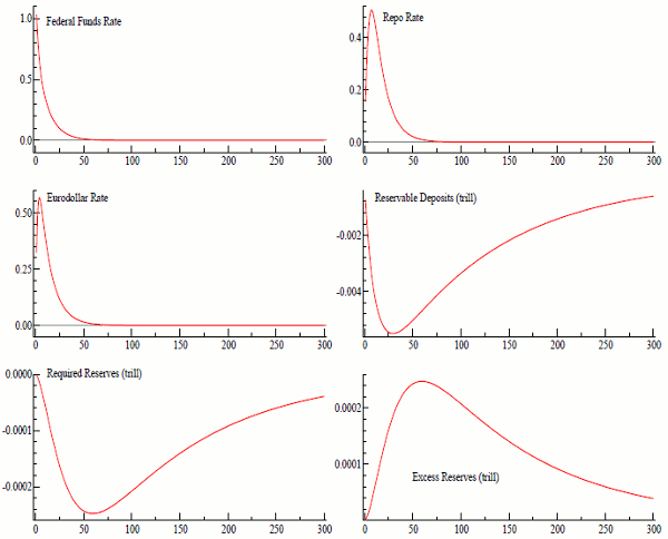
Reduced-form estimates cannot answer the following key questions: Is the equilibrium in the federal funds market stable? If so, is the adjustment to equilibrium smooth or oscillatory? Finally, how long does it take for the federal funds rate to reach a new steady state? To address these questions, we rely on the model's estimated impulse responses. Specifically, Figure 7 plots the impulse responses to an innovation in the federal funds rate. After the shock, the response of the federal funds rate falls quickly, with the rate reaching its new equilibrium in 60 days with the bulk of the adjustment taking place within the first week. The other overnight rates also increase and reach their equilibrium in about 60 days.25 The innovation in the federal funds rate also lowers reservable deposits and required reserves, which raises excess reserves and tends to dampen the increase in the federal funds rate.
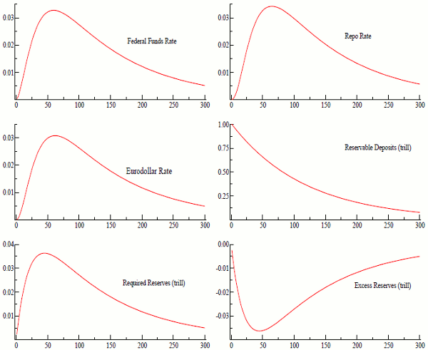
Figure 8 plots the impulse responses to an innovation in reservable deposits. After the shock, the response of these deposits falls as the federal funds rate increases. These deposits reach their new equilibrium in about a year but half of the adjustment is reached after 100 days. The increase in required reserves lowers excess reserves about one-for-one, which, in turn, raises the federal funds rate. This increase is transmitted to the other interest rates, pushing them in the same direction; their responses die out after one year.
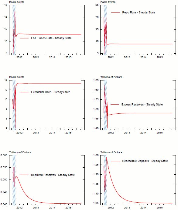
These impulse responses suggest that the model is stable, and so we now examine whether the steady state implied by these responses is meaningful from an economic standpoint. To this end, we conduct dynamic simulations through December 2015 under the assumption that residuals are zero and that all exogenous variables remain constant at their last historical value for estimation (March 30, 2012).26 As Figure 9 shows, the model reaches a meaningful steady state by the beginning of 2013 with reasonable values for the endogenous variables: the federal funds rate is about 11 basis points and the historical spreads among funding rates are preserved. That is, the rate on secured funding (repo rate) is below the rates on unsecured funding (the federal funds and Eurodollar rates).
4 Monetary Policy Simulations
Based on our estimation results, we conduct dynamic simulations to assess the effects of monetary policy changes on overnight interest rates. In the following, we first describe the impact of changes in the supply of reserve balances on short-term interest rates in normal times--that is, the effect of changes in conventional monetary policy, with reserve balances at their pre-crisis level.27 Second, we analyze the effects of further monetary policy accommodation on short-term interest rates, either through another round of large-scale asset purchases or a cut in the IOER rate. Third, assuming a path for the removal of monetary policy accommodation by the Federal Reserve that is consistent with the June 2011 FOMC exit principles (FOMC (2011b)), we provide the first empirical assessment of the response of short-term interest to this exit strategy.
4.1 Effects of Conventional Monetary Policy
Prior to the financial crisis, temporary open market operations--primarily repurchase agreements--were the Federal Reserve's primary means for day-to-day monetary policy implementation. The Federal Reserve conducted these operations to align the supply of reserve balances with the demand for these balances to attain the target federal funds rate set by the FOMC.28
Changes in the supply of reserve balances affect the federal funds rate, all else equal. This effect can be quantified by determining the slope of the demand curve for reserves. The estimation result in Table 4 (row 6, column 5) suggests that reserve balances
adjust nearly one-for-one to changes in repurchase agreements (RP). The effect of a change in the Federal Reserve's repurchase agreements on the federal funds rate is
![]() (row 6, column 5 in Table 4), which takes into account the effect of a change in reserve balances on the the federal
funds rate. As discussed previously, the magnitude of the effect depends on the level of the federal funds rate. Assuming a federal funds rate of 4%, a $10 billion increase in
(row 6, column 5 in Table 4), which takes into account the effect of a change in reserve balances on the the federal
funds rate. As discussed previously, the magnitude of the effect depends on the level of the federal funds rate. Assuming a federal funds rate of 4%, a $10 billion increase in ![]() , which
raises reserve balances by nearly the same amount, lowers the federal funds rate by approximately 4 basis points. Clearly, in an environment with lower overnight interest rates, an equally-sized increase in
, which
raises reserve balances by nearly the same amount, lowers the federal funds rate by approximately 4 basis points. Clearly, in an environment with lower overnight interest rates, an equally-sized increase in ![]() has a much smaller effect on the federal funds rate.
has a much smaller effect on the federal funds rate.
4.2 Effects of Additional Unconventional Monetary Policy
We now use the model to examine the effects of further policy accommodation by the Federal Reserve. When asked at the semi-annual testimony to Congress on July 17, 2012 about options for further monetary policy easing, Federal Reserve Chairman Bernanke mentioned various actions the Federal Reserve has at its disposal. In this study, we are assessing two of these options: (1) another round of large-scale asset purchases and (2) lowering the interest rate on excess reserves.29
First, we simulate a hypothetical increase in ![]() . In our model, the federal funds rate declines as the supply of reserves increases with the expansion in
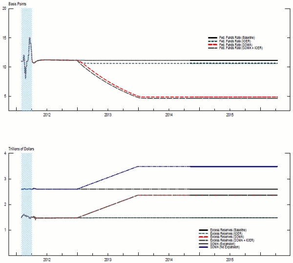
. In our model, the federal funds rate declines as the supply of reserves increases with the expansion in ![]() (the paths of SOMA and excess reserves under the different scenarios are shown in the bottom panel of Figure 10). In our simulation, for simplicity, we assume that
(the paths of SOMA and excess reserves under the different scenarios are shown in the bottom panel of Figure 10). In our simulation, for simplicity, we assume that ![]() increases by $900 billion over a period of one year, starting in January 2013, the date when the Maturity Extension Program (MEP) will be completed.30 The simulations reveal that the gradual expansion in
increases by $900 billion over a period of one year, starting in January 2013, the date when the Maturity Extension Program (MEP) will be completed.30 The simulations reveal that the gradual expansion in ![]() lowers the federal funds rate gradually from 11 basis points to
5 basis points after one year, as indicated by the dashed line in Figure 10. The seemingly small response owes to the non-linearity of the model, as reflected in the low starting value of the federal funds rate. Indeed, as shown in equation (18), the response of the federal funds rate to a small change in
lowers the federal funds rate gradually from 11 basis points to
5 basis points after one year, as indicated by the dashed line in Figure 10. The seemingly small response owes to the non-linearity of the model, as reflected in the low starting value of the federal funds rate. Indeed, as shown in equation (18), the response of the federal funds rate to a small change in ![]() is
is
![]() .
.
Second, we simulate a hypothetical reduction in the IOER rate of 10 basis points, from the current level of 25 basis points, on January 1, 2013. The downward pressure of a cut in the IOER rate of 10 basis point on the federal funds rates is very small, leaving the federal funds rate nearly
unchanged (see the short-dashed line in Figure 10). Again, the insignificance of this effect is not surprising in the context of the non-linearity of the model. Specifically, equation (20) indicates that
![]() , that is, if the initial value of the federal funds rate is low, so will be its response to a change in the IOER rate.
, that is, if the initial value of the federal funds rate is low, so will be its response to a change in the IOER rate.
Finally, we combine these hypothetical policy actions. As indicated by the long-dashed line in Figure 10, the combined action--expanding ![]() and cutting the IOER
rate--lowers the federal funds rate by a marginal amount relative to the baseline.
and cutting the IOER
rate--lowers the federal funds rate by a marginal amount relative to the baseline.
4.3 Effects of the Removal of Unconventional Monetary Policy
In the June 2011 FOMC minutes, the Committee stated its exit principles (FOMC (2011b)). These principles are listed, verbatim, in column 1 of Table 5. Greatly simplified, the stated principles envision an exit strategy implemented in four phases:
- Stop reinvestments of securities.
- Implement temporary reserve-drainage operations (e.g., expand the Term Deposit Facility (TDF) or conduct reverse repurchase agreements (RRP)).
- Increase policy rates.
- Sell SOMA securities.
When removing the monetary accommodation, the FOMC has stated a preference for the federal funds rate to evolve in a corridor between the discount rate and the IOER rate:
"&lsqb#lbrack;...] Most of these participants indicated that they preferred that monetary policy eventually operate through a corridor-type system in which the federal funds rate trades in the middle of a range, with the IOER rate as the floor and the discount rate as the ceiling of the range, as opposed to a floor-type system in which a relatively high level of reserve balances keeps the federal funds rate near the IOER rate. [...]" (FOMC (2011a))
However, the principles do not include detailed information about the magnitude of the actions, their pace, or their timing. This absence of detailed information raises two relevant questions. First, does the sequence specified by the principles affect the dynamic path of the federal funds rate? Second, does the federal funds rate settle in a corridor as possibly preferred by the FOMC? We address these questions through model simulations, carried out under several assumptions.31 These hypothetical assumptions, which are one of many possible ways the FOMC can carry out these principles, are shown in column 2 of Table 5.32 We begin with changes in one policy at a time to assess the importance of non-linearities. We find that there are important non-linearities, which leads us to examine their implications for the principles' sequencing. Finally, we change several policy variables at once to assess the feasibility of a corridor system.
4.3.1 Non-Linearities
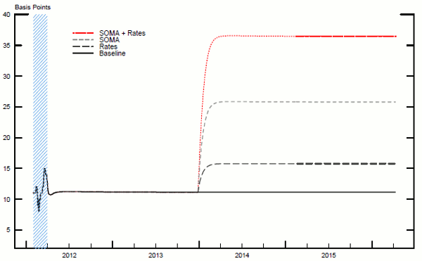
The first scenario is a hypothetical, instantaneous reduction in ![]() of $900 billion. As indicated by the short-dashed line in Figure 11, the federal funds rate
reaches a steady state of 25 basis points over a short period of time. This result suggests that, all other policy variables unchanged, a substantial reduction in
of $900 billion. As indicated by the short-dashed line in Figure 11, the federal funds rate
reaches a steady state of 25 basis points over a short period of time. This result suggests that, all other policy variables unchanged, a substantial reduction in ![]() is needed to raise the
federal funds rate to the level of the IOER rate, which so far has provided only an imperfect floor for the federal funds rate.33 This results is consistent
with Bech & Klee (2011) who suggest that a large amount of reserve balances needs to be drained before DIs begin to enter the federal funds market to meet their financing needs, and the the IOER rate may be used as a monetary policy tool to help guide the federal
funds rate.
is needed to raise the
federal funds rate to the level of the IOER rate, which so far has provided only an imperfect floor for the federal funds rate.33 This results is consistent
with Bech & Klee (2011) who suggest that a large amount of reserve balances needs to be drained before DIs begin to enter the federal funds market to meet their financing needs, and the the IOER rate may be used as a monetary policy tool to help guide the federal
funds rate.
The second scenario is a hypothetical increase of 25 basis points in the discount rate (![]() ). As indicated by the dashed line in Figure 11, this action
raises the federal funds rate by about 5 basis points implying a less than proportional response because of the non-linearities. Recall, however, that this response is sensitive to the initial values of the two interest rates.
). As indicated by the dashed line in Figure 11, this action
raises the federal funds rate by about 5 basis points implying a less than proportional response because of the non-linearities. Recall, however, that this response is sensitive to the initial values of the two interest rates.
To assess how important non-linearities are in the model, we include a third policy action, in which the above decline in ![]() and the increase in the discount rate are implemented
simultaneously. The dotted line in Figure 11 plots the response of the federal funds rate to that combination of policy actions. If the model were linear, then the response from the combination of actions should be approximately equal to the sum of the responses of the
separate actions. As shown in Figure 11, the sum of the interest-rate responses to the two shocks is 20 basis points whereas the response associated with an implementation of both shocks at once is 25 basis points. In other words, the responsiveness of the federal funds
rate to shocks is non-linear. This finding suggests that the sequencing of policy actions might affect the profile of the adjustment process.
and the increase in the discount rate are implemented
simultaneously. The dotted line in Figure 11 plots the response of the federal funds rate to that combination of policy actions. If the model were linear, then the response from the combination of actions should be approximately equal to the sum of the responses of the
separate actions. As shown in Figure 11, the sum of the interest-rate responses to the two shocks is 20 basis points whereas the response associated with an implementation of both shocks at once is 25 basis points. In other words, the responsiveness of the federal funds
rate to shocks is non-linear. This finding suggests that the sequencing of policy actions might affect the profile of the adjustment process.
4.3.2 Sequencing
To study the implications of the principles' stated sequencing for the federal funds rate, we use the two policy actions already considered but change the timing of their implementation:
- Schedule A:
- An instantaneous reduction in SOMA by $0.9 trillion on January 1, 2014.
- An increase in the discount rate of 25 basis points on January 1, 2014.
- Schedule B:
- An instantaneous reduction in SOMA by $0.9 trillion on January 1, 2015.
- An increase in the discount rate of 25 basis points on January 1, 2014.
- Schedule C:
- An instantaneous reduction in SOMA by $0.9 trillion on January 1, 2014.
- An increase in the discount rate of 25 basis points on January 1, 2015.
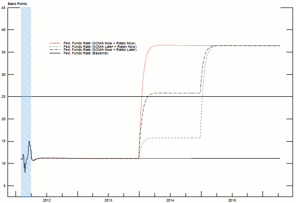
The simulations reveal that, although the steady state of the federal funds rate is invariant to changing the sequencing of the shocks, the adjustment profile of the federal funds rate is not (Figure 12). The sequencing from Schedule C (a reduction in ![]() followed by an increase in the discount rate) raises the federal funds rate in two steps of roughly equal size (the dashed line) whereas the reverse sequencing results in a muted initial response of the
federal funds rate but a sharp increase in the federal funds rate later (the short-dashed line). The optimal choice depends on policy makers' preferences.
followed by an increase in the discount rate) raises the federal funds rate in two steps of roughly equal size (the dashed line) whereas the reverse sequencing results in a muted initial response of the
federal funds rate but a sharp increase in the federal funds rate later (the short-dashed line). The optimal choice depends on policy makers' preferences.
4.3.3 Feasibility of a Corridor
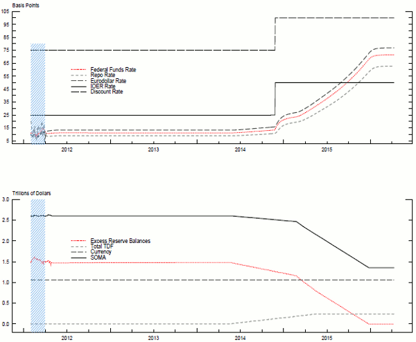
The process of reversing the accommodative stance of monetary policy begins with the implementation of principles 2 and 3 in Table 5. Starting in June 2014, we assume that the FOMC stops reinvestments, which translates into a reduction in
![]() of $20 billion per month until March 2015. Further, we assume that the FOMC expands the Term Deposit Facility (TDF): Deposits in this facility increase by $10 billion in bi-weekly auctions,
which end in June 2015; the bottom panel of Figure 13 shows the profile of these two variables. Note that the combined reserve drainage amounts through the TDF and SOMA reductions that we chose is below the pace of the increase in reserves during the second large-scale asset
purchase program.34 The implementation of the next principle is assumed to involve an increase in both the discount rate and the
IOER rate. We assume this increase to be 25 basis points (see the top panel of Figure 13) and to take place in December 2014. The implementation of the last principle involves an active reduction of
of $20 billion per month until March 2015. Further, we assume that the FOMC expands the Term Deposit Facility (TDF): Deposits in this facility increase by $10 billion in bi-weekly auctions,
which end in June 2015; the bottom panel of Figure 13 shows the profile of these two variables. Note that the combined reserve drainage amounts through the TDF and SOMA reductions that we chose is below the pace of the increase in reserves during the second large-scale asset
purchase program.34 The implementation of the next principle is assumed to involve an increase in both the discount rate and the
IOER rate. We assume this increase to be 25 basis points (see the top panel of Figure 13) and to take place in December 2014. The implementation of the last principle involves an active reduction of ![]() . We assume a gradual reduction of $5 billion per day starting in March 2015 and ending in December 2015.
. We assume a gradual reduction of $5 billion per day starting in March 2015 and ending in December 2015.
Based on these assumptions, ![]() declines from $2.6 trillion in 2012 to $1.4 trillion by the beginning of 2016 and excess reserves decline from $1.5 trillion to almost zero over the same
period, while term deposits increase to $300 billion (bottom panel of Figure 13). Under these assumptions, our model projects that the federal funds rate rises gradually, reaching 70 basis points by the end of 2015, with the historical spreads between overnight interest rates
preserved (top panel of Figure 13). These results suggest that, without drastic policy actions, the federal funds rate can move into a corridor between the IOER rate and the discount rate, consistent with most FOMC members' preference, as stated in the April 2011 FOMC minutes
(FOMC (2011a)).
declines from $2.6 trillion in 2012 to $1.4 trillion by the beginning of 2016 and excess reserves decline from $1.5 trillion to almost zero over the same
period, while term deposits increase to $300 billion (bottom panel of Figure 13). Under these assumptions, our model projects that the federal funds rate rises gradually, reaching 70 basis points by the end of 2015, with the historical spreads between overnight interest rates
preserved (top panel of Figure 13). These results suggest that, without drastic policy actions, the federal funds rate can move into a corridor between the IOER rate and the discount rate, consistent with most FOMC members' preference, as stated in the April 2011 FOMC minutes
(FOMC (2011a)).
5 Conclusion
In this study, we model the interplay between the Federal Reserve's balances sheet and overnight interest rates, while allowing for interdependencies among overnight funding rates. In particular, we formulate a system of equations modeling the federal funds rate, the repo rate, the Eurodollar rate, reserve balances held by depository institutions, and demand deposit holdings. We rely on full-information methods for parameter estimation, recognizing the interdependencies among overnight funding rates and accounting for possible simultaneity biases. We use this framework to assess the effects of both conventional and unconventional monetary policy changes on short-term interest rates. As for unconventional policy actions, we estimate the impact of further policy accommodation by the Federal Reserve and the removal of the policy accommodation currently in place.
According to our results, in the current environment with quite elevated levels of excess reserve balances by historical standards, the effect of further monetary policy accommodation, in the form of large-scale asset purchases or a cut in the IOER rate, on short-term interest rates is limited because these rates are already close to zero. Moreover, assuming a path for the removal of monetary policy accommodation that is consistent with the June 2011 FOMC exit principles, we project that the accommodative stance of monetary policy is effectively removed and short-term funding markets return to a more normal functioning. Under our assumptions, the federal funds rate is projected to increase to 70 basis points by 2016, while excess reserves of DIs decline to a level close to that observed prior to the crisis. Finally, we document that, while the steady state is invariant to the order of policy changes, the sequencing of different policy measures in an exit strategy matters for the profile of the response of the federal funds rate.
Bibliography
Journal of Finance 66(4):1109-1139.
Journal of Monetary Economics 58(5):415-431.
Finance and Economics Discussion Series 2012-21, Federal Reserve Board.
American Economic Review 94(2):85-90.
Brookings Papers on Economic Activity 2004(2):1-78.
Journal of Money, Credit and Banking 38(4):901-920.
Journal of Money, Credit, and Banking 40(1):1-24.
Forthcoming Finance and Economics Discussion Series paper, Federal Reserve Board.
Topics in Macroeconomics 3(1):1534-5998.
http://www.federalreserve.gov/monetarypolicy/fomcminutes20110427.htm.
http://www.federalreserve.gov/monetarypolicy/fomcminutes20110622.htm.
Journal of Financial Economics 104(3):425-451.
Journal of Political Economy 104(1):26-56.
American Economic Review 87(1):80-97.
Journal of Macroeconomics 32(3):713-731.
Journal of Banking & Finance 35(12):3292-3299.
Annual Report by the Markets Group of the Federal Reserve Bank of New York.
McGraw-Hill, New York, 4 edn.
Figure 1: Federal Funds Rate, Reserve Balances of Depository Institutions, and Securities Held by the Federal Reserve
| (1) Federal Funds Market | (2) Eurodollar Market | (3) Repo Market | |
|---|---|---|---|
| Borrowers | Depository Institutions | Depository Institutions | Depository Institutions, Broker Dealers |
| Lenders | Depository Institutions, Broker Dealers, GSEs | Money Market Funds Financial and Nonfinancial Lenders | Money Market Funds Securities, Lenders, GSEs |
Column (1) of the table outlines the principles of the exit strategy as described in the historical minutes of the June 2011 FOMC meeting. Column (2) lists the implementation of theses principles in our simulations. Column (3) contains the time line for various steps of the exit strategy. This table reports the FIML parameter estimates of equations (9)-(14). All interest rates and personal income are in logarithms. Standard errors are reported in squared brackets.
| Fed. Funds Rate: Fed. Funds Rate (-1) | 0.798 |
| Fed. Funds Rate: Fed. Funds Rate (-1) (Standard Error) | [0.016] |
| Fed. Funds Rate: Constant | -0.061 |
| Fed. Funds Rate: Constant (Standard Error) | [0.006] |
| Fed. Funds Rate: Repo Rate | 0.016 |
| Fed. Funds Rate: Repo Rate (Standard Error) | [0.005] |
| Fed. Funds Rate: Eurdol. Rate | 0.091 |
| Fed. Funds Rate: Eurdol. Rate (Standard Error) | [0.014] |
| Fed. Funds Rate: Disc. Rate | 0.120 |
| Fed. Funds Rate: Disc. Rate (Standard Error) | [0.009] |
| Fed. Funds Rate: IOER | 0.048 |
| Fed. Funds Rate: IOER (Standard Error) | [0.025] |
| Fed. Funds Rate: Excess Reserves | -0.093 |
| Fed. Funds Rate: Excess Reserves (Standard Error) | [0.010] |
| Fed. Funds Rate: Memo: RMSE | 3.88bp |
| Repo Rate: Repo Rate (-1) | 0.773 |
| Repo Rate: Repo Rate (-1) (Standard Error) | [0.014] |
| Repo Rate: Constant | -0.034 |
| Repo Rate: Constant (Standard Error) | [0.006] |
| Repo Rate: Fed. Funds Rate | 0.104 |
| Repo Rate: Fed. Funds Rate (Standard Error) | [0.045] |
| Repo Rate: Eurdol. Rate | 0.143 |
| Repo Rate: Eurdol. Rate (Standard Error) | [0.047] |
| Repo Rate: Memo: RMSE | 7.40bp |
| Eurdol. Rate: Eurdol. Rate (-1) | 0.634 |
| Eurdol. Rate: Eurdol. Rate (-1) (Standard Error) | [0.018] |
| Eurdol. Rate: Constant | 0.024 |
| Eurdol. Rate: Constant (Standard Error) | [0.003] |
| Eurdol. Rate: Fed. Funds Rate | 0.308 |
| Eurdol. Rate: Fed. Funds Rate (Standard Error) | [0.019] |
| Eurdol. Rate: Repo Rate | 0.035 |
| Eurdol. Rate: Repo Rate (Standard Error) | [0.010] |
| Eurdol. Rate: Memo: RMSE | 2.38bp |
| Res. Deposits: Res. Deposits (-1) | 0.992 |
| Res. Deposits: Res. Deposits (-1) (Standard Error) | [0.003] |
| Res. Deposits: Constant | -0.050 |
| Res. Deposits: Constant (Standard Error) | [0.026] |
| Res. Deposits: Fed. Funds Rate | -0.001 |
| Res. Deposits: Fed. Funds Rate (Standard Error) | [0.000] |
| Res. Deposits: Income | 0.006 |
| Res. Deposits: Income (Standard Error) | [0.003] |
| Res. Deposits: Memo: RMSE | $23bn |
| Rq. Reserves: Rq. Reserves (-1) | 0.955 |
| Rq. Reserves: Rq. Reserves (-1) (Standard Error) | [0.007] |
| Rq. Reserves: Constant | -0.001 |
| Rq. Reserves: Constant (Standard Error) | [0.000] |
| Rq. Reserves: Res. Deposits | 0.002 |
| Rq. Reserves: Res. Deposits (Standard Error) | [0.000] |
| Rq. Reserves: Memo: RMSE | $0.58bn |
| 1/9/2003 - 7/31/2008 Coefficient | 1/9/2003 - 7/31/2008 Std.Error | 7/31/2008 - 3/30/2012 Coefficient | 7/31/2008 - 3/30/2012 Std.Error | 1/9/2003 - 3/30/2012 Coefficient | 1/9/2003 - 3/30/2012 Std.Error | |
| Fed. Funds Rate: Fed. Funds Rate (-1) | 0.764 | 0.067 | 0.712 | 0.025 | 0.798 | 0.016 |
| Fed. Funds Rate: Repo Rate | 0.012 | 0.009 | 0.022 | 0.008 | 0.016 | 0.005 |
| Fed. Funds Rate: Eurdol. Rate | 0.180 | 0.064 | 0.071 | 0.022 | 0.091 | 0.014 |
| Fed. Funds Rate: Excess Reserves | -0.206 | 0.187 | -0.244 | 0.024 | -0.093 | 0.010 |
| Fed. Funds Rate: Discount Rate | 0.055 | 0.009 | 0.222 | 0.019 | 0.120 | 0.009 |
| Fed. Funds Rate: IOER | -- | -- | 0.041 | 0.036 | 0.048 | 0.025 |
| Fed. Funds Rate: Constant | -0.029 | 0.006 | -0.035 | 0.011 | -0.061 | 0.006 |
| Fed. Funds Rate: SER | 0.031 | 0.100 | 0.072 | |||
| Repo Rate: Repo Rate (-1) | 0.792 | 0.018 | 0.760 | 0.023 | 0.773 | 0.014 |
| Repo Rate: Fed. Funds Rate | 0.604 | 0.189 | 0.084 | 0.073 | 0.104 | 0.045 |
| Repo Rate: Eurdol. Rate | -0.389 | 0.177 | 0.159 | 0.079 | 0.143 | 0.047 |
| Repo Rate: Constant | -0.015 | 0.005 | -0.078 | 0.034 | -0.034 | 0.006 |
| Repo Rate: SER | 0.077 | 0.388 | 0.249 | |||
| Eurdol. Rate: Eurdol. Rate (-1) | 0.338 | 0.024 | 0.600 | 0.028 | 0.634 | 0.018 |
| Eurdol. Rate: Repo Rate | -0.035 | 0.008 | 0.043 | 0.017 | 0.035 | 0.010 |
| Eurdol. Rate: Fed. Funds Rate | 0.710 | 0.027 | 0.306 | 0.031 | 0.308 | 0.019 |
| Eurdol. Rate: Constant | -0.013 | 0.002 | -0.018 | 0.020 | 0.024 | 0.003 |
| Eurdol. Rate: SER | 0.030 | 0.219 | 0.144 | |||
| Res. Deposits: Res. Deposits (-1) | 0.959 | 0.007 | 0.975 | 0.008 | 0.992 | 0.003 |
| Res. Deposits: Federal Funds Rate | 0.000 | 0.001 | -0.003 | 0.001 | -0.001 | 0.000 |
| Res. Deposits: Income | -0.001 | 0.004 | 0.079 | 0.026 | 0.006 | 0.003 |
| Res. Deposits: Constant | 0.038 | 0.038 | -0.728 | 0.239 | -0.050 | 0.026 |
| Res. Deposits: SER | 0.010 | 0.015 | 0.012 | |||
| Rq. Reserves: Rq. Reserves (-1) | 0.976 | 0.006 | 0.933 | 0.013 | 0.955 | 0.007 |
| Rq. Reserves: Res. Deposits | -0.001 | 0.001 | 0.004 | 0.001 | 0.002 | 0.000 |
| Rq. Reserves: Constant | 0.001 | 0.000 | -0.001 | 0.000 | -0.001 | 0.000 |
| Rq. Reserves: SER | 0.001 | 0.002 | 0.001 |
| SOMA | Disc. Rate | IOER | Constant | Repos | Net Other | Currency | Income | |
| Fed. Funds Rate | -0.933 | 1.204 | 0.482 | -0.887 | -0.993 | 0.993 | 0.993 | 0.035 |
| Fed. Funds Rate (Standard Error) | [0.058] | [0.033] | [0.241] | [0.156] | [0.058] | [0.058] | [0.058] | [0.016] |
| Repo Rate | -0.981 | 1.265 | 0.507 | -1.045 | -0.981 | 0.981 | 0.981 | 0.037 |
| Repo Rate (Standard Error) | [0.064] | [0.044] | [0.254] | [0.168] | [0.064] | [0.064] | [0.064] | [0.017] |
| Eurdol. Rate | -0.881 | 1.136 | 0.455 | -0.783 | -0.881 | 0.881 | 0.881 | 0.033 |
| Eurdol. Rate (Standard Error) | [0.056] | [0.034] | [0.228] | [0.148] | [0.056] | [0.056] | [0.056] | [0.015] |
| Res. Deposits | 0.078 | -0.100 | -0.040 | -5.841 | 0.078 | -0.078 | -0.078 | 0.711 |
| Res. Deposits (Standard Error) | [0.021] | [0.027] | [0.023] | [2.977] | [0.021] | [0.021] | [0.021] | [0.319] |
| Rq. Reserves | 0.004 | -0.005 | -0.002 | -0.325 | 0.004 | -0.004 | -0.004 | 0.038 |
| Rq. Reserves (Standard Error) | [0.001] | [0.001] | [0.001] | [0.160] | [0.001] | [0.001] | [0.001] | [0.017] |
| Excess Reserves | 0.996 | 0.005 | 0.002 | 0.325 | 0.996 | -0.996 | -0.996 | -0.038 |
| Excess Reserves (Standard Error) | [0.001] | [0.001] | [0.001] | [0.160] | [0.001] | [0.001] | [0.001] | [0.017] |
| (1) Principle | (2) Implementation | (3) Time line | |
| 1 | The Committee will determine the timing and pace of policy normalization to promote its statutory mandate of maximum employment and price stability. | No change needed | -- |
| 2 | To begin the process of policy normalization, the Committee will likely first cease reinvesting some or all payments of principal on the securities holdings in the SOMA. | Reduction in SOMA of $20 billion per month | June 2014 - March 2015 |
| 3 | At the same time or sometime thereafter, the Committee will modify its forward guidance on the path of the federal funds rate and will initiate temporary reserve-draining operations aimed at supporting the implementation of increases in the federal funds rate when appropriate. | Initiation of TDF: Increase in Other Liabilities (OL) by $10 billion per biweekly auction | June 2014 - June 2015 |
| 4 | When economic conditions warrant, the Committee's next step in the process of policy normalization will be to begin raising its target for the federal funds rate, and from that point on, changing the level or range of the federal funds rate target will be the primary means of adjusting the stance of monetary policy. During the normalization process, adjustments to the interest rate on excess reserves and to the level of reserves in the banking system will be used to bring the funds rate toward its target. | Increase in IOER rate by 25 basis points and increase in the target federal funds rate to 50 basis points | December 2014 |
| 5 | Sales of agency securities from the SOMA will likely commence sometime after the first increase in the target for the federal funds rate. The timing and pace of sales will be communicated to the public in advance; that pace is anticipated to be relatively gradual and steady, but it could be adjusted up or down in response to material changes in the economic outlook or financial conditions. | Gradual Reduction of SOMA by $5 billion/day | March 2015 - December 2015 |
| 6 | Once sales begin, the pace of sales is expected to be aimed at eliminating the SOMA's holdings of agency securities over a period of three to five years, thereby minimizing the extent to which the SOMA portfolio might affect the allocation of credit across sectors of the economy. Sales at this pace would be expected to normalize the size of the SOMA securities portfolio over a period of two to three years. In particular, the size of the securities portfolio and the associated quantity of bank reserves are expected to be reduced to the smallest levels that would be consistent with the efficient implementation of monetary policy. | No change needed | -- |
| 7 | The Committee is prepared to make adjustments to its exit strategy if necessary in light of economic and financial developments. | No change needed | -- |
Footnotes
| (16) |
where
![]() is the vector of predictions for the endogenous variables,
is the vector of predictions for the endogenous variables,
![]() is the vector of exogenous variables, and
is the vector of exogenous variables, and
![]() and
and
![]() are matrices of estimated parameters. The associated deterministic long-run solution is
are matrices of estimated parameters. The associated deterministic long-run solution is
where
where ![]() is the last date of the estimation sample (March 30, 2012) and
is the last date of the estimation sample (March 30, 2012) and ![]() is the
simulation horizon, which is set to 1100 days. Return to Text
is the
simulation horizon, which is set to 1100 days. Return to Text
![\displaystyle \widehat{\mathbf{y}}_{t}=\left[ \mathbf{I-}\widehat{\mathbf{\mathbf{A}}}% \right] ^{-1}\cdot \widehat{\mathbf{B}}\mathbf{x}_{t}=\widehat{\Pi }\cdot \mathbf{x},](img58.gif)