
Board of Governors of the Federal Reserve System
International Finance Discussion Papers
Number 867r, March 2011 --- Screen Reader
Version*
Closing Large Open Economy Models**
NOTE: International Finance Discussion Papers are preliminary materials circulated to stimulate discussion and critical comment. References in publications to International Finance Discussion Papers (other than an acknowledgment that the writer has had access to unpublished material) should be cleared with the author or authors. Recent IFDPs are available on the Web at http://www.federalreserve.gov/pubs/ifdp/. This paper can be downloaded without charge from the Social Science Research Network electronic library at http://www.ssrn.com/.
Abstract:
A large class of international business cycle models admits multiple locally isolated deterministic steady states, if the elasticity of substitution between traded goods is sufficiently low. I explore the conditions under which such multiplicity occurs and characterize the dynamic properties in the neighborhood of each steady state. Models with standard incomplete markets, portfolio costs, a debt-elastic interest rate, or an overlapping generations framework allow for multiple steady states, if the model features multiple steady states under financial autarchy. If the excess demand for the foreign traded good is increasing in the good's own price in a given steady state, the equilibrium dynamics around this steady state are unbounded. Otherwise, the dynamics are bounded and unique. By contrast, with Uzawa-type preferences, the steady state is always unique and the associated equilibrium dynamics are always bounded and unique. The same results obtain under complete markets.
Keywords: Stationarity, incomplete markets, open economy, multiple equilibria
JEL classification: D51, F41
1 Introduction
The class of international business cycle models nested in the framework of Corsetti, Dedola, and Leduc (2008) admits multiple steady states with zero net foreign asset holdings, if the elasticity of substitution between traded goods is sufficiently low. This paper explores the conditions under which such multiplicity occurs and characterizes the models' dynamic properties in the neighborhood of each steady state.
Equilibrium multiplicity is a pervasive feature of models with heterogenous agents. To build intuition consider the case of a static two-country endowment economy with two traded goods that are imperfect substitutes as in Kehoe (1991) and Mas-Colell, Whinston, and Green (1995). For simplicity, let the countries be mirror images of each other with respect to preferences and endowments. One equilibrium always features a relative price of the traded goods equal to unity. With home bias in consumption and a low elasticity of substitution between the traded goods, two more equilibria occur. If the price of the domestic good is high relative to the price of the foreign good, domestic agents are wealthy compared to foreign agents. Under a low elasticity of substitution, foreigners are willing to give up most of their good in order to consume at least some of the domestic good, and domestic agents end up consuming most of both goods. The reverse is true as well. Foreign agents consume most of the goods, if the foreign good is expensive in relative terms.
This intuition carries over to richer models of the international business cycle that feature international borrowing and lending, endogenous production, intertemporal savings and investment decisions, or non-traded goods. For these models to feature multiple steady states with zero net foreign assets under an otherwise standard calibration the elasticity of substitution between traded goods has to lie below 0.5.1 Whereas in most studies the elasticity of substitution between traded goods and the trade (price) elasticity coincide, the two concepts differ in the model of Corsetti, Dedola, and Leduc (2008) due to the presence of non-traded distribution services. If the model is parameterized as in Corsetti, Dedola, and Leduc (2008), multiple steady states occur for an elasticity of substitution between traded goods around unity, although the implied trade elasticity lies in the neighborhood of 0.5.
For a symmetric parameterization of the model I generally find three steady states. However, the model by Corsetti, Dedola, and Leduc (2008) can be shown to have at least five steady states for some parameterizations.2
The multiplicity of the steady state price vector occurs whether international financial markets are absent from the model or one focuses on an incomplete financial markets framework with zero net foreign assets in steady state.3 This problem is unrelated to the issues about incomplete markets models addressed in Schmitt-Grohé and Uribe (2003) and many others. In standard incomplete markets model with one non-state-contingent bond the deterministic steady state of the net foreign asset position is not determined and the dynamics of the net foreign asset position as derived from a linear approximation of the model around a deterministic steady state are not stationary.4 Absent arbitrage opportunities, the price of the non-state-contingent bond implies that expected marginal utility growth is equalized across countries. In the deterministic steady state, this condition contains no information about the steady state values of the system and the system of equilibrium conditions becomes underdetermined. In particular, any net foreign asset position is compatible with a steady state.
To determine the steady state position of net foreign assets and to remove the non-stationarity of its dynamics, I modify the original model similar to Schmitt-Grohé and Uribe (2003) by allowing for portfolio costs, a debt-elastic interest rate, or an endogenous discount factor. This list is augmented by the overlapping generations structure of Weil (1989) as implemented in Ghironi (2006) and Ghironi (2008). I show that the choice of a stationarity inducing device is not innocuous as it affects both the number of steady states in a low elasticity environment and the dynamics of the model around a steady state.
With portfolio costs, agents face a non-zero cost for bond
holdings that differs from a reference level for international bond
holdings specified exogenously by the researcher. Furthermore, the
steady state is unique and stable only if the model with financial
autarchy (or equivalently with incomplete markets and a zero net
foreign asset position) has a unique steady state. If the original
model has ![]() steady states, the model with portfolio
costs has
steady states, the model with portfolio
costs has ![]() steady states. Those steady states for
which the excess demand of the foreign good is decreasing in its
relative price are associated with unique and locally bounded
equilibrium dynamics. If the excess demand function is increasing
in its relative price in a given steady state, the local
equilibrium dynamics are not bounded. Interestingly, if multiple
steady states occur under a symmetric calibration, it is typically
the symmetric steady state that is associated with unbounded
dynamics. Similar results are obtained for the cases of the
debt-elastic interest rate and the overlapping generations
framework.
steady states. Those steady states for
which the excess demand of the foreign good is decreasing in its
relative price are associated with unique and locally bounded
equilibrium dynamics. If the excess demand function is increasing
in its relative price in a given steady state, the local
equilibrium dynamics are not bounded. Interestingly, if multiple
steady states occur under a symmetric calibration, it is typically
the symmetric steady state that is associated with unbounded
dynamics. Similar results are obtained for the cases of the
debt-elastic interest rate and the overlapping generations
framework.
Following Uzawa (1968), when the discount factor is assumed to be endogenous, an agent's rate of time preference is strictly decreasing in the agent's utility level. With strictly concave preferences and technologies the relative price of traded goods is uniquely pinned down under endogenous discounting given the function of the discount factor. The net foreign asset position is merely a residual. The equilibrium dynamics in the neighborhood of the unique steady state are always unique and locally bounded irrespective of the number of steady states in the original model with incomplete markets.5
Schmitt-Grohé and Uribe (2003) also analyze the case of complete markets. In this case, the net foreign asset position is a residual that does not enter the equilibrium dynamics as a state variable. The steady state of such a model is always unique and the associated equilibrium dynamics are unique and bounded.
Both Schmitt-Grohé and Uribe (2003) and Kim and Kose (2003) find that for the case of a small open economy the various approaches imply virtually identical dynamics. However, generalizing this finding to richer models as made by many researchers, may not be appropriate. Boileau and Normandin (2008) extend the analysis in Schmitt-Grohé and Uribe (2003) to a two-country model with one homogeneous good. Quantitative differences can occur in their setup depending on the persistence of technology shocks.
This paper exclusively analyzes the local dynamics around a given steady state. However, in the presence of multiple steady states, global solution techniques may find richer dynamics than local solution techniques. Bodenstein (2010) presents an analysis of the global dynamics in the model of Backus, Kehoe, and Kydland (1995) under endogenous discounting when the elasticity of substitution between traded goods is sufficiently low.
Remains to address the empirical relevance of models with low trade and substitution elasticities. For aggregate data Whalley (1984) reports a trade elasticity of 1.5. Hooper, Johnson, and Marquez (1998) report a short-run trade elasticity of 0.6 for the U.S. and values between 0 and 0.6 for the remaining G7 countries, while Taylor (1993) finds a short-run trade elasticity of 0.22. Using lower levels of aggregation, Broda and Weinstein (2006) report mean estimates for the elasticity of substitution for various pairs of traded goods between 4 and 6.
Applied macroeconomic studies, have commonly parameterized the substitution elasticity between traded goods at a value between 1 and 1.5 (see e.g. Backus, Kehoe, and Kydland (1995), Chari, Kehoe, and McGrattan (2002), and Heathcote and Perri (2002)). However, in line with the macroeconometric evidence, various authors have recently argued in favor of low values of the trade elasticity which coincides with the elasticity of substitution between traded goods for these studies. Heathcote and Perri (2002), Benigno and Thoenissen (2008) and Collard and Dellas (2007) show improved model performance with respect to key features of the international business cycle when allowing for substitution elasticities below 0.5.
Burstein, Neves, and Rebelo (2003), Corsetti and Dedola (2005), and Corsetti, Dedola, and Leduc (2008) refrain from assuming such low substitution elasticities directly, but instead introduce distribution costs in terms of non-traded goods to obtain a low implied value of the trade elasticity despite allowing the elasticity of substitution between traded goods to be around unity. The model in Corsetti, Dedola, and Leduc (2008) successfully addresses two important puzzles in international economics: the high volatility of the real exchange rate relative to fundamentals and the observed negative correlation between the real exchange rate and relative consumption (Backus and Smith (1993)).
As Kollmann (2006) shows, a low elasticity of substitution between traded goods may also be responsible for the apparent home bias in equity holdings. Rabanal and Tuesta (2010) estimate a DSGE model with sticky prices using a Bayesian approach. Their median estimates for the elasticity of substitution range from 0.01 to 0.91for different specifications of their model. Lubik and Schorfheide (2006) estimate the elasticity of substitution to be around 0.4.
The remainder of the paper is structured as follows. Section 2 introduces the issues considered in this paper in a simple model. Section 3 lays out the general model, which is parameterized in Section 4. Steady state multiplicity is discussed in Section 5, while the local dynamics of the model are discussed in Section 6. Concluding remarks are offered in Section 7. The paper is accompanied by a separate Technical Appendix.
2 Simple Example
Consider a two-country, two-good endowment economy with incomplete international financial markets. The two countries are each inhabited by a continuum of identical agents of measure 1. This model extends the introductory example in Corsetti, Dedola, and Leduc (2008) to a dynamic environment. I first illustrate under what restrictions on the value of the elasticity of substitution between traded goods the model admits multiple deterministic steady states. Second, I relate steady state multiplicity to the question when the local dynamics around a given steady state are locally bounded or unbounded.
Each period ![]() , agents in country
, agents in country ![]() obtain
obtain ![]() units of the traded good
units of the traded good
![]() . Agents consume both the home and the
foreign good and maximize their expected discounted lifetime
utility. The only asset that trades internationally is one
non-state-contingent bond. More formally, a representative agent
faces:
. Agents consume both the home and the
foreign good and maximize their expected discounted lifetime
utility. The only asset that trades internationally is one
non-state-contingent bond. More formally, a representative agent
faces:
 |
(1) |
| (2) |
All variables are expressed in per capita terms. ![]() is the consumption of good
is the consumption of good ![]() by agents of
country
by agents of
country ![]() .
. ![]() is the price of good
is the price of good
![]() .
. ![]() denotes holdings of a
non-state-contingent bond with price
denotes holdings of a
non-state-contingent bond with price ![]() . To rule
out Ponzi-schemes, I assume that agents face an upper bound for
borrowing
. To rule
out Ponzi-schemes, I assume that agents face an upper bound for
borrowing ![]() that is large enough to
never bind in this application. The aggregate consumption good
that is large enough to
never bind in this application. The aggregate consumption good
![]() satisfies:
satisfies:
![$\displaystyle \left[ \left( \alpha _{i1}^{T}\right) ^{\frac{1}{ \varepsilon ^{T}}}\left( c_{i1,t+j}\right) ^{\frac{\varepsilon ^{T}-1}{ \varepsilon ^{T}}}+\left( \alpha _{i2}^{T}\right) ^{\frac{1}{\varepsilon ^{T} }}\left( c_{i2,t+j}\right) ^{\frac{\varepsilon ^{T}-1}{\varepsilon ^{T}}} \right] ^{\frac{\varepsilon ^{T}}{\varepsilon ^{T}-1}},$](img39.gif) |
(3) |
with
![]() for
for ![]() and
and ![]() . The elasticity of substitution
between the two traded goods is denoted by
. The elasticity of substitution
between the two traded goods is denoted by
![]() . Market clearing
requires:
. Market clearing
requires:
| (4) | |
| (5) | |
| (6) |
The price of the aggregate consumption good in country 1 is taken to be the numéraire.
2.1 Steady State Multiplicity
Under the assumption that the net foreign asset position is zero
in steady state (![]() ), this model can display
multiple distinct steady states if the elasticity of substitution
between the two traded goods is sufficiently low. The relative
price
), this model can display
multiple distinct steady states if the elasticity of substitution
between the two traded goods is sufficiently low. The relative
price
![]() constitutes a steady state
equilibrium, if the excess demand function for good 2
satisfies:
constitutes a steady state
equilibrium, if the excess demand function for good 2
satisfies:
| (7) |
Applying standard fixed-point theorems, it can be shown that a
steady state exists for this model. Furthermore, by virtue of the
index theorem, see Kehoe (1991) and Mas-Colell, Whinston, and Green (1995),
the number of steady state equilibria needs to be odd. Furthermore,
if the slope of the excess demand function is positive for a given
steady state value of ![]() with zero net foreign assets,
there must be at least two more values of
with zero net foreign assets,
there must be at least two more values of ![]() for which
for which
![]() .
.
Figure 1: Excess Demand Function and Steady State Multiplicity
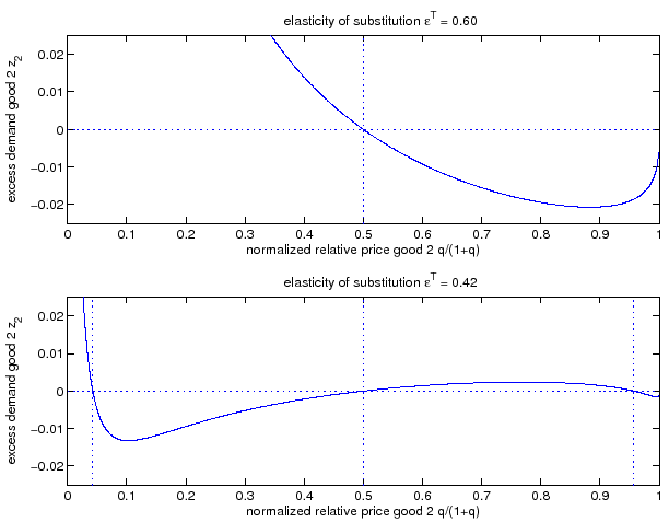
Notes: The figure plots the excess
demand function for good 2 as a function of the normalized relative
price ![]() with
with
![]() ,
,
![]() , and
, and
![]() . The solid line depicts the
excess demand function. The dotted vertical lines indicate the
zeros of the excess demand function. For
. The solid line depicts the
excess demand function. The dotted vertical lines indicate the
zeros of the excess demand function. For
![]() , the unique zero features
, the unique zero features
![]() . For
. For
![]() , the three zeros occur at
, the three zeros occur at
![]() equal to 0.043,
0.500, and 0.957,
respectively.
equal to 0.043,
0.500, and 0.957,
respectively.
To advance the analysis, I set
![]() ,
,
![]() , for
, for
![]() and
and ![]() and fix
and fix
![]() in steady state. Under
these assumptions, one steady state always features
in steady state. Under
these assumptions, one steady state always features ![]() ,
i.e.,
,
i.e.,
![]() , irrespective of the value
of
, irrespective of the value
of ![]() . Figure 1 plots the excess
demand for good 2 as a function the normalized price
. Figure 1 plots the excess
demand for good 2 as a function the normalized price
![]() for a high and a low value of
for a high and a low value of
![]() . The remaining parameter values
are
. The remaining parameter values
are
![]() ,
,
![]() , and
, and
![]() . In the case of
. In the case of
![]() , the excess demand function
equals zero only for
, the excess demand function
equals zero only for ![]() . Furthermore, the slope of
the excess demand function is negative at
. Furthermore, the slope of
the excess demand function is negative at ![]() . For
the lower value of
. For
the lower value of ![]() of 0.42, the
slope of the excess demand function is positive at the steady state
equilibrium with
of 0.42, the
slope of the excess demand function is positive at the steady state
equilibrium with ![]() . Consequently, there are two more
price equilibria: one for
. Consequently, there are two more
price equilibria: one for
![]() and the other one for
and the other one for
![]() .
.
As shown in Appendix A, the slope of the excess demand function in a deterministic steady state is given by:

Balanced trade in steady state implies
![]() and
the slope of the excess demand function for good 2 is
then positive at
and
the slope of the excess demand function for good 2 is
then positive at ![]() , if:
, if:
 |
(8) |
Thus, the model features multiple steady states, whenever condition (8) is satisfied. For the parameterization underlying Figure 1 the threshold value for the elasticity of substitution at which steady state multiplicity occurs is 0.4444. The associated change in the sign of the slope of the excess demand function from negative to positive at a low value of the substitution elasticity lies behind what Corsetti, Dedola, and Leduc (2008) term "the negative transmission mechanism" and allows their model to be a candidate solution to the Backus-Smith puzzle.6
2.2 Local Equilibrium Dynamics
The incomplete markets model outlined in the previous section features two well-known problems if the decision rules are derived from a linear approximation around a deterministic steady state. First, any value of the net foreign asset position is compatible with a steady state. Second, the model is not stationary as the net foreign asset position follows a unit root process.
The first order conditions with respect to bond holdings imply, that expected marginal utility growth expressed in a common good needs to be equalized across countries:
![$\displaystyle \mathbb{E}_{t+j} \left[ \beta \left(\frac{c^T_{1,t+1+j}}{c^T_{1,t+j}}\right)^{-1}\right] = \mathbb{E}_{t+j}\left[\beta \left(\frac{c^T_{2,t+1+j}}{c^T_{2,t+j}}\right)^{-1} \frac{rer_{t+j}}{rer_{t+1+j}}\right].$](img95.gif) |
(9) |
In steady state, equation (9) reduces to an
identity, leading to a system of ![]() unknown endogenous
variables, but
unknown endogenous
variables, but ![]() equations. It is common practice
to exogenously specify the steady state value of the net foreign
asset position. For the remainder of the paper, I will assume that
the net foreign position is zero in steady state. Thus, the model
with incomplete markets has the same steady states as a model
without internationally traded assets.
equations. It is common practice
to exogenously specify the steady state value of the net foreign
asset position. For the remainder of the paper, I will assume that
the net foreign position is zero in steady state. Thus, the model
with incomplete markets has the same steady states as a model
without internationally traded assets.
However, imposing the steady state level of net foreign assets
exogenously does not remove the unit root of the net foreign asset
position in the approximate model. Following among others
Schmitt-Grohé and Uribe (2003), I introduce portfolio costs
to render the net foreign asset position stationary.7 Households incur the cost
 for holding or issuing international debt. These costs are rebated
lump-sum to the households. As portfolio costs are zero whenever
the net foreign asset position is zero, the steady states in the
model with portfolio costs are the same as in the model described
in the previous subsection.
To study the dynamics around a given steady state, Appendix A shows
that the unique state variable
![]() satisfies the
system:8
satisfies the
system:8
 |
(10) |
![]() represents
the slope of the excess demand function for good 2. The term
represents
the slope of the excess demand function for good 2. The term
![]() is always negative in steady
state. and the sign of
is always negative in steady
state. and the sign of
![]() is
immaterial for the subsequent analysis. The portfolio costs imposed
on the agents are represented by the parameter:
is
immaterial for the subsequent analysis. The portfolio costs imposed
on the agents are represented by the parameter:
![\begin{displaymath} \check{\gamma} =\frac{\gamma}{\beta ^{2}\Phi _{1}\left( q\right) }\left[ 1+\frac{1}{q}\right]>0. \end{displaymath}](img107.gif) |
(11) |
The term
![]() is positive (negative), whenever
is positive (negative), whenever
![]() is
negative (positive) in the deterministic steady state around which
the model is approximated.
is
negative (positive) in the deterministic steady state around which
the model is approximated.
The following theorem shows that steady states for which the excess demand function is upward-sloping display unbounded dynamics under the portfolio cost approach.
Theorem 1 Around a given steady state, the eigenvalues of the dynamic system associated with the portfolio cost model λ1 and λ2 satisfy:
1. For 3. For
![]() ,
, ![]() and
and  . Thus, bond holdings follow a unit-root process (restating the non-stationarity problem under incomplete markets).
2. For ![]() , and
, and  (a downward sloping excess demand function),
 ![]() and
and  . Thus, the dynamics around the point of approximation are locally unique and bounded.
![]() , and
, and  (an upward sloping excess demand function),
 ![]() and
and  . Thus, teh dynamics around the point of approximation are not bounded.
Proof. The proof follows directly from teh characteristic equation associated with the approximate system:
 |
(12) |
If the number of eigenvalues larger than one in absolute value exceeds (falls short of) the number of state vairables, the equilibrium dynamics are not bounded (indeterminate). If the number of such eigenvalues coincides with the number of state variables, the dynamics are unique and bounded.
An alternative approach of rendering the net foreign asset position stationary is due to Uzawa (1968). As shown in Section 5, the steady state under endogenous discounting is always unique for a given parameterization of the model. Replacing ![]() in equation (1) by
in equation (1) by
![]() with
with
![]() and, to ease
exposition, assuming that agents do not internalize the effects of
their current choices on future discount factors, one obtains:
and, to ease
exposition, assuming that agents do not internalize the effects of
their current choices on future discount factors, one obtains:
Theorem 2 Around the unique steady state, the eigenvalues of the dynamic system with an endogenous discount factor satisfy ![]() and
and  . Thus, the equilibrium dynamics around a steady state are always locally unique and bounded irrespective of the slope of the excess demand function in this steady state.
Proof. The proof follows directly from the characteristic equation associated with the approximate system:
 |
(13) |
where the additional term ![]() is always positive.
is always positive.
2.3 Intuition
Multiplicity of steady states In the model with portfolio costs, the steady state interest rate
equals
![]() . Hence, no country has an
incentive to borrow or lend in steady state. All equilibria of the
financial autarchy case are therefore valid steady states since
they are compatible with
. Hence, no country has an
incentive to borrow or lend in steady state. All equilibria of the
financial autarchy case are therefore valid steady states since
they are compatible with ![]() .
.
The model of endogenous discounting, however, dictates that for
a given functional choice of the discount factor
![]() in the steady
state. Uniqueness of the steady state price
in the steady
state. Uniqueness of the steady state price ![]() follows promptly: suppose that another price
vector
follows promptly: suppose that another price
vector ![]() that constitutes a steady state with
that constitutes a steady state with
![]() is also a steady state of the
model with endogenous discounting. Let
is also a steady state of the
model with endogenous discounting. Let ![]() , which would imply that overall consumption
in country 1 exceeds overall consumption in country
2, i.e.,
, which would imply that overall consumption
in country 1 exceeds overall consumption in country
2, i.e.,
![]() . Thus, country
1 agents are willing to borrow resources at
an interest rate of
. Thus, country
1 agents are willing to borrow resources at
an interest rate of
![]() while country
2 agents only demand
while country
2 agents only demand
![]() .
Hence, country
.
Hence, country ![]() finds it optimal to borrow from
country 2 violating
finds it optimal to borrow from
country 2 violating ![]() .
.
Stability of steady states The logic behind the stability of the unique steady state in the
model with endogenous discounting is closely related to the
argument about its uniqueness. Assume that ![]() is below
its steady state value. This implies that consumption in country
1 (2) is above (below) its steady
state value. Suppose, that the relative price is even lower in the
next period, suggesting that the economy moves away from the steady
state. This implies an increasing (decreasing) consumption profile
in country 1 (2). In addition, the discount
factor in country 1 (2) falls (rises). Hence, the
price of the non-state-contingent bond falls in country 1 but rises in country 2. Obviously, the
opposite movement of bond prices is inconsistent with the absence
of arbitrage dictated by the risk sharing condition. Hence, if
is below
its steady state value. This implies that consumption in country
1 (2) is above (below) its steady
state value. Suppose, that the relative price is even lower in the
next period, suggesting that the economy moves away from the steady
state. This implies an increasing (decreasing) consumption profile
in country 1 (2). In addition, the discount
factor in country 1 (2) falls (rises). Hence, the
price of the non-state-contingent bond falls in country 1 but rises in country 2. Obviously, the
opposite movement of bond prices is inconsistent with the absence
of arbitrage dictated by the risk sharing condition. Hence, if
![]() is below its steady state value at time
is below its steady state value at time
![]() ,
, ![]() must rise in
must rise in ![]() and the economy converges to its unique steady state.
and the economy converges to its unique steady state.
Consider the case of a steady state with
![]() in
the bond economy with portfolio costs. The price of bonds consists
of two pieces: the intertemporal marginal rate of substitution and
the derivative of the portfolio costs. First, if
in
the bond economy with portfolio costs. The price of bonds consists
of two pieces: the intertemporal marginal rate of substitution and
the derivative of the portfolio costs. First, if ![]() is slightly below its steady state value, overall consumption in
country 1 (2) is above (below) its
corresponding steady state value. Stability of the steady state
requires
is slightly below its steady state value, overall consumption in
country 1 (2) is above (below) its
corresponding steady state value. Stability of the steady state
requires ![]() to rise and
to rise and ![]() to fall
over time. As a result, the intertemporal marginal rate of
substitution in country 1 (2) rises (falls), which leads
to a divergence of bond prices. Second, when
to fall
over time. As a result, the intertemporal marginal rate of
substitution in country 1 (2) rises (falls), which leads
to a divergence of bond prices. Second, when ![]() rises, bond holdings and the derivative of the portfolio costs
fall. This effect on bond prices is negative in both countries, but
it is stronger in country 2 since portfolio
costs are measured in terms of each country's good. This second
effect operates towards a rise of the bond price in country
2 relative to country 1.
However, the change in bond holdings is small owing to the fact
that the excess demand function is fairly flat around such a steady
state. Hence, bond prices would drift apart if a steady state with
sign
rises, bond holdings and the derivative of the portfolio costs
fall. This effect on bond prices is negative in both countries, but
it is stronger in country 2 since portfolio
costs are measured in terms of each country's good. This second
effect operates towards a rise of the bond price in country
2 relative to country 1.
However, the change in bond holdings is small owing to the fact
that the excess demand function is fairly flat around such a steady
state. Hence, bond prices would drift apart if a steady state with
sign
 was
stable. Hence, such a steady must be associated by unbounded
dynamics.
Using the model by Corsetti, Dedola, and Leduc (2008), the remainder of this paper explores the conditions for steady state multiplicity and the local dynamics under different stationarity inducing devices.
3 General Model
Each of the two countries ![]() produces two
goods. The first good is traded internationally without trade
frictions (traded good), while the other good is not traded
(non-traded good). The home and foreign traded goods are imperfect
substitutes in a household's utility function. The traded and the
non-traded goods are produced by perfectly competitive firms and
production requires the use of labor and capital. As an important
deviation from earlier work, Corsetti, Dedola, and Leduc (2008) assume
that consumption of traded goods requires non-traded distribution
services as input.
produces two
goods. The first good is traded internationally without trade
frictions (traded good), while the other good is not traded
(non-traded good). The home and foreign traded goods are imperfect
substitutes in a household's utility function. The traded and the
non-traded goods are produced by perfectly competitive firms and
production requires the use of labor and capital. As an important
deviation from earlier work, Corsetti, Dedola, and Leduc (2008) assume
that consumption of traded goods requires non-traded distribution
services as input.
3.1 Standard Incomplete Markets Economy
The subsequent analysis explores the implications of different assumptions about international financial markets in the presence of multiple steady states. In laying out the full model, I assume that international financial markets are incomplete in the sense that the only asset that trades internationally is one non-state-contingent bond.
3.1.1 Households
The representative household in country ![]() maximizes its expected discounted lifetime utility subject to its
budget constraint. All variables are expressed in per household
units:
maximizes its expected discounted lifetime utility subject to its
budget constraint. All variables are expressed in per household
units:
|
(14) |
|
(15) |
| (16) |
where ![]() ,
, ![]() ,
, ![]() and
and ![]() denote final consumption, final
investment, labor, and capital, respectively.
denote final consumption, final
investment, labor, and capital, respectively. ![]() is the price of the final consumption good,
is the price of the final consumption good,
![]() is the price of the final
investment good,
is the price of the final
investment good, ![]() is the price of the traded good
produced by country
is the price of the traded good
produced by country ![]() ,
, ![]() and
and
![]() are the nominal rental rate of
capital and the nominal wage. Assuming local ownership of firms,
are the nominal rental rate of
capital and the nominal wage. Assuming local ownership of firms,
![]() are the profits of the traded and
non-traded goods producers that are located in country
are the profits of the traded and
non-traded goods producers that are located in country ![]() .
. ![]() denotes holdings of the
non-state-contingent bond.
denotes holdings of the
non-state-contingent bond. ![]() is the price of
this bond. To rule out Ponzi-schemes, I assume that agents face an
upper bound for borrowing
is the price of
this bond. To rule out Ponzi-schemes, I assume that agents face an
upper bound for borrowing ![]() that is
large enough to never bind in this application.
that is
large enough to never bind in this application.
3.1.2 Firms
Both the producers of traded and non-traded goods utilize labor
and capital and act in perfectly competitive factor and product
markets. Technologies are of the constant elasticity of
substitution type. Since capital is owned by households and rented
out to firms, the maximization problem of a traded goods producer
from country ![]() can be written as:
can be written as:
 |
(17) |
where the production technology satisfies:
|
(18) |
|
(19) |
with
![]() . Let
. Let
![]() denote the supply of the traded
good. The problem of non-traded goods producers is analogous with
variables and parameters carrying the superscript
denote the supply of the traded
good. The problem of non-traded goods producers is analogous with
variables and parameters carrying the superscript ![]() rather than
rather than ![]() . Because of the normalization choice
for factor prices, the objective function of such firms is given
by:
. Because of the normalization choice
for factor prices, the objective function of such firms is given
by:
 |
(20) |
3.1.3 Trade and Aggregation
Households in country ![]() consume the final
consumption good
consume the final
consumption good ![]() and purchase the final
investment good
and purchase the final
investment good ![]() . Shipping of the traded goods
is costless.
. Shipping of the traded goods
is costless.
Consumption good A household in country ![]() purchases
purchases ![]() units of the traded good of
country 1,
units of the traded good of
country 1, ![]() units of the traded
good of country 2, and
units of the traded
good of country 2, and ![]() units
of the non-traded good. The three types of goods are combined to
form the final consumption good according to:
units
of the non-traded good. The three types of goods are combined to
form the final consumption good according to:
![$\displaystyle \left[ \left( \alpha _{i1}^{T}\right) ^{\frac{1}{ \varepsilon_{i} ^{T}}}\left( c_{i1,t+j}\right) ^{\frac{\varepsilon_{i} ^{T}-1}{ \varepsilon_{i} ^{T}}}+\left( \alpha _{i2}^{T}\right) ^{\frac{1}{\varepsilon_{i} ^{T} }}\left( c_{i2,t+j}\right) ^{\frac{\varepsilon_{i} ^{T}-1}{\varepsilon_{i} ^{T}}} \right] ^{\frac{\varepsilon_{i} ^{T}}{\varepsilon_{i} ^{T}-1}},$](img204.gif) |
(21) | ||
![$\displaystyle \left[ \left( \alpha _{i1}^{N}\right) ^{\frac{1}{\varepsilon_{i} ^{N}}}\left( c_{i,t+j}^{T}\right) ^{\frac{\varepsilon_{i} ^{N}-1}{\varepsilon_{i} ^{N}}}+\left( \alpha _{i2}^{N}\right) ^{\frac{1}{\varepsilon_{i} ^{N}}}\left( c_{i,t+j}^{N}\right) ^{\frac{\varepsilon_{i} ^{N}-1}{\varepsilon_{i} ^{N}}}\right] ^{ \frac{\varepsilon_{i} ^{N}}{\varepsilon_{i} ^{N}-1}},$](img207.gif) |
(22) |
with
![]() and
and
![]() for
for ![]() ,
, ![]() . These quasi shares in the
aggregators are assumed to sum up to 1.
. These quasi shares in the
aggregators are assumed to sum up to 1.
![]() is the substitution
elasticity between the traded goods aggregate and the non-traded
good in country
is the substitution
elasticity between the traded goods aggregate and the non-traded
good in country ![]() .
.
![]() is the substitution
elasticity between the home and foreign traded goods. As in
Burstein, Neves, and Rebelo (2003) and Corsetti, Dedola, and Leduc (2008), the
consumption of traded goods requires distribution services.
Consuming one unit of any traded good goes along with a cost of
is the substitution
elasticity between the home and foreign traded goods. As in
Burstein, Neves, and Rebelo (2003) and Corsetti, Dedola, and Leduc (2008), the
consumption of traded goods requires distribution services.
Consuming one unit of any traded good goes along with a cost of
![]() units of the country's non-traded
good. Thus, minimizing the costs for
units of the country's non-traded
good. Thus, minimizing the costs for ![]() units of
the final consumption good requires solving the problem:
units of
the final consumption good requires solving the problem:
 |
(27) |
subject to (21) and (22).
Investment good The final investment good is an aggregate of traded goods only. In combining the two traded goods, the household solves:
|
(24) |
![$\displaystyle x_{i,t+j}=\left[ \left( \alpha _{i1}^{I}\right) ^{\frac{1}{\varepsilon_{i} ^{I}} }\left( x_{i1,t+j}\right) ^{\frac{\varepsilon_{i} ^{I}-1}{\varepsilon_{i} ^{I}} }+\left( \alpha _{i2}^{I}\right) ^{\frac{1}{\varepsilon_{i} ^{I}}}\left( x_{i2,t+j}\right) ^{\frac{\varepsilon_{i} ^{I}-1}{\varepsilon_{i} ^{I}}}\right] ^{ \frac{\varepsilon_{i} ^{I}}{\varepsilon_{i} ^{I}-1}},$](img220.gif) |
(25) |
with
![]() for
for ![]() ,
, ![]() and
and
![]() . The
substitution elasticity between traded goods for investment is
denoted by
. The
substitution elasticity between traded goods for investment is
denoted by
![]() .
.
Relative prices For later reference, define the following
relative prices: the relative price of country 2's
good to country 1's good
![]() ,
the relative price of the non-traded good
,
the relative price of the non-traded good
 , the
inverse relative price of final consumption
![]() , the
inverse relative price of final investment
, the
inverse relative price of final investment
![]() . Thus, the
consumption real exchange rate is given by
. Thus, the
consumption real exchange rate is given by
![]() . In
solving the model, aggregate consumption in country 1
is set to be the numéraire, i.e.,
. In
solving the model, aggregate consumption in country 1
is set to be the numéraire, i.e., ![]() .
.
3.1.4 Market Clearing and Equilibrium
Goods market clearing requires:
 |
(26) |
| (27) |
for ![]() at all
at all ![]() . With
. With
![]() , differences in relative population
size are captured by
, differences in relative population
size are captured by ![]() . Factor market clearing
requires:
. Factor market clearing
requires:
| (28) | |
| (29) |
for ![]() at all
at all ![]() . The bond
market clears if:
. The bond
market clears if:
 |
(30) |
A competitive equilibrium is consequently defined as:
Definition 1 A competitive equilibrium is a collection of allocations
![]() ,
, ![]() ,
, ![]() ,
, ![]() ,
, ![]() , xi1,t+j,
, xi1,t+j, ![]() ,
, ![]() ,
, ![]() ,
, ![]() ,
, ![]() ,
, ![]() ,
, ![]() ,
, ![]() ,
, ![]() ,
, ![]() ,
, ![]() , prices
, prices ![]() ,
, ![]() ,
, ![]() ,
, ![]() ,
, ![]() ,
, ![]() ,
, ![]() ,
, ![]() and profits
and profits ![]() , for i = 1,2 and all j, such that (i) for every household the allocations solve a household's maximization problem for given prices, (ii) for every firm profits are maximized, adn (iii) the markets for labor, capital, goods, and bonds clear.
, for i = 1,2 and all j, such that (i) for every household the allocations solve a household's maximization problem for given prices, (ii) for every firm profits are maximized, adn (iii) the markets for labor, capital, goods, and bonds clear.
3.1.5 Trade Elasticity
Absent distribution services (![]() for
for
![]() ), the elasticity of substitution
between traded goods coincides with the trade (price) elasticity.
However, this is not the case for
), the elasticity of substitution
between traded goods coincides with the trade (price) elasticity.
However, this is not the case for ![]() ;
the price of the home good relative to the foreign good at the
consumer level no longer matches the terms of trade, i.e., the
relative price between traded goods. The first order condition of
the consumer problem implies:
;
the price of the home good relative to the foreign good at the
consumer level no longer matches the terms of trade, i.e., the
relative price between traded goods. The first order condition of
the consumer problem implies:
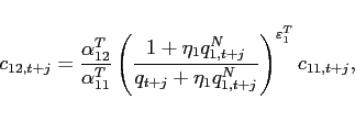 |
(31) |
or after linearizing around a deterministic steady state:
![\begin{displaymath} \hat{c}_{11,t+j}-\hat{c}_{12,t+j}=\frac{\varepsilon _{1}^{T}}{1+\eta _{1}\frac{q_{1}^{N}}{q}}\hat{q}_{t+j}-\left[ \frac{1}{1+\eta _{1}q_{1}^{N}}-\frac{1}{ q+\eta _{1}q_{1}^{N}}\right] \varepsilon _{1}^{T}\eta _{1}q_{1}^{N}\hat{q} _{1,t+j}^{N}, \end{displaymath}](img261.gif) |
(37) |
where ![]() denotes the log-linear deviation of
variable
denotes the log-linear deviation of
variable ![]() from its steady state value.
from its steady state value.
Corsetti, Dedola, and Leduc (2008) refer to
 as
the trade elasticity. In addition to the elasticity of substitution
between traded goods
![]() , the trade elasticity
depends on the endogenous steady state values of both the relative
price of traded goods
, the trade elasticity
depends on the endogenous steady state values of both the relative
price of traded goods ![]() and the relative price of
non-traded goods
and the relative price of
non-traded goods ![]() .
.
3.2 Assumptions on International Financial Markets
I investigate the following deviations from the standard incomplete markets model that render the net foreign asset position stationary and determine its steady state:
- Agents face portfolio costs for holding/issuing bonds as in
Heathcote and Perri (2002) and Schmitt-Grohé and Uribe (2003). The budget constraint (15) changes to:


(33)
The portfolio cost function satisfies
 ,
,
 , and
, and
 for
for  and
and
 for
for  , and
, and
 .
.
 is a lump-sum transfer in the
amount of the collected fees. Consequently, condition (9) changes to:
![$\displaystyle \mathbb{E}_{t+j} \left[ \beta \frac{U_{c}\left(c_{1,t+1+j},l_{1,t+1+j}\right) }{U_{c}\left(c_{1,t+j},l_{1,t+j} \right)}\right]= \mathbb{E}_{t+j}\left[\beta \frac{U_{c}\left(c_{2,t+1+j},l_{2,t+1+j}\right) }{U_{c}\left(c_{2,t+j},l_{2,t+j} \right)} \frac{rer_{t+j}}{rer_{t+1+j}}\right]$](img279.gif)

(34) - The interest rate is debt-elastic as in Boileau and Normandin (2008), [Devereux and Smith 2007], and Schmitt-Grohé and Uribe (2003). The interest rate differential between the two
countries is given by:

(35)
with . The function
 satisfies
 and
and
 .
.  is a reference level of debt for country
1, which is set to zero. When country
1 is a net borrower, it faces an interest
rate that is higher than the interest rate in country 2. When country 1 is a lender, it receives an
interest rate that is lower. Condition (9) changes to:
![$\displaystyle \Psi \left( b_{1,t+1+j}-\bar{b}_{1}\right) \mathbb{E}_{t+j} \left[ \beta \frac{U_{c}\left(c_{1,t+1+j},l_{1,t+1+j}\right) }{U_{c}\left(c_{1,t+j},l_{1,t+j} \right)}\right]$](img291.gif)
![$\displaystyle = \mathbb{E}_{t+j}\left[\beta \frac{U_{c}\left(c_{2,t+1+j},l_{2,t+1+j}\right) }{U_{c}\left(c_{2,t+j},l_{2,t+j} \right)} \frac{rer_{t+j}}{rer_{t+1+j}}\right].$](img292.gif)
(36)
- To break Ricardian equivalence, the representative household
assumption is replaced by an overlapping generations framework
based on Weil (1989) and Ghironi (2006). Each period, the
population in country
 grows at the constant growth
rate
  . As newborn households do not hold assets,
the net foreign asset position is zero in the deterministic steady
state. More details are provided in Appendix B.
- The discount factor is endogenous as in Uzawa (1968), Mendoza
(1991), Corsetti, Dedola, and Leduc (2008), and Schmitt-Grohé and Uribe (2003). The problem of a household is given by:


(37) ![$\displaystyle \theta _{i,t+1+j} =\beta _{i} \left[ U\left( c_{i,t+j} ,l_{i,t+j} \right) \right] \theta _{i,t+j},$](img297.gif)
(38)
and equations (15) and (16) . The discount factor is assumed to be decreasing with the level of utility, i.e., . As in
Schmitt-Grohé and Uribe (2003), I lay out the case when
agents do not internalize the effects of time
  choices on the discount factor in future periods. Condition
(9)
changes to:
![$\displaystyle \mathbb{E}_{t+j} \left[ \beta_{1} \left[ U\left( c_{1,t+j} ,l_{1,t+j} \right) \right] \frac{U_{c}\left(c_{1,t+1+j},l_{1,t+1+j}\right) }{U_{c}\left(c_{1,t+j},l_{1,t+j} \right)}\right]$](img302.gif)
![$\displaystyle = \mathbb{E}_{t+j}\left[\beta_{2} \left[ U\left( c_{2,t+j} ,l_{2,t+j} \right) \right] \frac{U_{c}\left(c_{2,t+1+j},l_{2,t+1+j}\right) }{U_{c}\left(c_{2,t+j},l_{2,t+j} \right)} \frac{rer_{t+j}}{rer_{t+1+j}}\right].$](img303.gif)
(39)
The subsequent analysis also considers the case when agents internalize the effects of their choices on the discount factor.
- For completeness, I also investigate the case of complete
international financial markets, i.e., agents have access to a full
set of state-contingent claims. Efficient risk sharing implies that
the marginal utilities expressed in a common good are equalized
across countries subject to a constant
 :
:

(40)
where is determined by the allocations and
prices at time
  :
:

(41)
In the first three approaches, the wedge between expected
marginal utility growth in the two countries is eliminated in a
deterministic steady state only for ![]() . Under
endogenous discounting, condition (39) requires that
. Under
endogenous discounting, condition (39) requires that
![]() in steady state. With concave utility and technology functions and
in steady state. With concave utility and technology functions and
![]() being strictly increasing in
being strictly increasing in
![]() , the allocations and prices are
directly pinned down by this condition. The net foreign asset
position is then determined from the goods market clearing
condition in order to be compatible with these steady state
allocations and prices. As, in principle, the steady state net
foreign asset position may differ from zero in this model, I
restrict attention to parameterizations of the endogenous discount
factor such that the model implies the same steady states as the
original model, i.e., net foreign assets are zero in steady state.
Similarly, under complete markets the unique steady state for a
given value of
, the allocations and prices are
directly pinned down by this condition. The net foreign asset
position is then determined from the goods market clearing
condition in order to be compatible with these steady state
allocations and prices. As, in principle, the steady state net
foreign asset position may differ from zero in this model, I
restrict attention to parameterizations of the endogenous discount
factor such that the model implies the same steady states as the
original model, i.e., net foreign assets are zero in steady state.
Similarly, under complete markets the unique steady state for a
given value of ![]() may not imply zero net
foreign assets. Thus, I restrict attention to those value of
may not imply zero net
foreign assets. Thus, I restrict attention to those value of
![]() that imply the same steady states as
the original model.
that imply the same steady states as
the original model.
4 Parameterizations
Overall, I consider five models. Model I is a simple production economy without capital and traded goods only. Model II introduces endogenous capital formation. Model III allows for capital and non-traded goods.
Table 1a. Calibration of Baseline Model: Parameters Constant Across Models
| Description | Symbol | Value |
|---|---|---|
| Elasticity Between k and l Non-Traded Goods (Cobb-Douglas) | 0.00 | |
| Elasticity Between k and l Traded Goods (Cobb-Douglas) | 0.00 | |
| Depreciation Rate of Capital | 0.025 | |
| Elasticity Between Non-Traded Goods | | 0.74 |
| Elasticity Between Traded Goods Consumption | | 0.85 |
| Elasticity Between Traded Goods Investment | | 0.85 |
| Relative Population Size | 1.00 | |
| Discount Factor | 0.99 | |
| Intertemporal Consumption Elasticity | 2.00 | |
| (a) Cobb-Douglas Preferences: Weight on Consumption | 0.34 | |
| (a) Cobb-Douglas Preferences: Weight on Leisure | 0.66 | |
| (b) Additive Separable Preferences: Labor Supply Elasticity | -5.00 | |
| (b) Additive Separable Preferences: Weight Labor Disutility | 5.00 |
Table 1b. Calibration of Baseline Model: Parameters Varying Across Models
| Description | Symbol | Model: I | Model: II | Model: III | Model: IV | Model: V |
|---|---|---|---|---|---|---|
| Weight on Labor in Production of Non-Traded Good | n.a. | n.a. | n.a. | 0.560 | 0.560 | |
| Weight on Labor in Production of Traded Good | 1.000 | 0.610 | 0.610 | 0.610 | 0.610 | |
| Distribution Cost in Terms of Non-Traded Good | n.a. | n.a. | 0.000 | 1.090 | 1.090 | |
| (a) Cobb-Douglas Preferences: Weight Own Traded Good in Consumption | 0.938 | 0.938 | 0.910 | 0.720 | 0.910 | |
| (a) Cobb-Douglas Preferences: Weight Own Traded Good in Investment | 1.000 | 0.938 | 0.910 | 1.000 | 0.855 | |
| (a) Cobb-Douglas Preferences: Weight Overall Traded Good | 1.000 | 1.000 | 0.550 | 0.550 | 0.550 | |
| (b) Additive Separable Preferences: Weight Own Traded Good in Consumption | 0.945 | 0.945 | 0.924 | 0.720 | 0.905 | |
| (b) Additive Separable Preferences: Weight Own Traded Good in Investment | 1.000 | 0.945 | 0.924 | 1.000 | 0.905 | |
| (b) Additive Separable Preferences: Weight Overall Traded Good | 1.000 | 1.000 | 0.550 | 0.550 | 0.550 |
The fourth model is identical to the model presented in Corsetti, Dedola, and Leduc (2008), i.e., consumption of traded goods requires the use of non-traded distribution services. In contrast to models II and III, investment features complete home bias. Relative to model IV, model V relaxes the assumption of complete home bias in investment. As models IV and V feature non-zero distribution costs, the trade elasticity is not fully determined by the elasticity of substitution between traded goods.
Table 1 summarizes the parameterizations for the five different models. To the extent possible, parameters are set equal across models. Parameter differences reflect the differences in model features. For each model, the quasi shares in equation (21) and (22) are adjusted to obtain an import to GDP ratio of 6.2 percent as in Corsetti, Dedola, and Leduc (2008).
Household preferences are described either by a Cobb-Douglas function:
 |
(42) |
or an additive separable utility function:
 |
(43) |
The functional forms for the stationarity inducing devices are:
- for the portfolio costs approach

(44)
- for a debt-elastic interest rate

(45)
- for endogenous discounting under Cobb-Douglas preferences

(46)
under additive separable preferences

(47)
5 Steady State Multiplicity
I first compute the set of steady states under the assumption
that financial markets are absent at the international level, i.e.,
![]() for all
for all ![]() , before
commenting on the remaining market arrangements outlined in Section 3.2.
, before
commenting on the remaining market arrangements outlined in Section 3.2.
Absent dynamics all the endogenous variables can be expressed as
functions of the relative price
![]() . An equilibrium with zero
net foreign asset holdings is then characterized by any value of
. An equilibrium with zero
net foreign asset holdings is then characterized by any value of
![]() that implies zero excess demand
that implies zero excess demand ![]() for the traded good of country 2:
for the traded good of country 2:
| (48) | |
| (49) |
Thus, the steady states can be computed reliably by searching
over a one-dimensional grid on the interval
[0, 1] for the normalized
relative price ![]() .
.
5.1 Steady States Under Financial Autarchy
Figure 2 plots the set of
steady state equilibrium prices for different values of the
elasticity of substitution between traded goods in the five models
for both Cobb-Douglas preferences and additive separable
preferences. Each model displays a unique price equilibrium with
![]()
 , if
the substitution elasticity is high. When the two traded goods are
assumed to be less substitutable, multiple steady states arise. The
two asymmetric steady states feature a relative price
 ![]() close to zero or one, respectively, and are hard
to detect in practice.
close to zero or one, respectively, and are hard
to detect in practice.
To understand how multiple equilibria arise at low values of the elasticity of substitution consider the case of the model without capital and traded goods only (model I). If the price of good 1 is high relative to the price of good 2 (lower branch), the value of country 1's production is high relative to country 2's. As labor supply is assumed to be fairly inelastic, overall production is price inelastic, as well. Agents in country 2 are willing to pay the high price for good 1 and country 1 ends up consuming most of the two goods. Similar logic applies when q is much larger than 1 (upper branch) with the roles of countries 1 and 2 being reversed. The middle equilibrium, which always exists, is the symmetric equilibrium with q = 1.
Figure 2. Steady State Multiplicity for Different Values of the Elasticity of Substitution
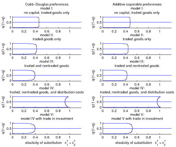
Notes: Set of normalized relative
prices ![]() that constitute a steady state absent
financial markets as a function of the elasticity of substitution
between traded goods. The (symmetric) parameterizations of models I
to V are given in Table 1.
that constitute a steady state absent
financial markets as a function of the elasticity of substitution
between traded goods. The (symmetric) parameterizations of models I
to V are given in Table 1.
As can be seen in Figure 2 and Table 2 the
threshold value of the substitution elasticity
![]() for which equilibrium
multiplicity occurs is model dependent, but it does not vary much
across the two specifications of household preferences for standard
parameterizations. Keeping trade shares constant at an import to
GDP ratio of 6.2 percent across models,
for which equilibrium
multiplicity occurs is model dependent, but it does not vary much
across the two specifications of household preferences for standard
parameterizations. Keeping trade shares constant at an import to
GDP ratio of 6.2 percent across models,
![]() falls when capital
accumulation and non-traded goods are introduced. For model II,
with an endogenous capital stock, a country carries a lower capital
stock and reduces production, if the relative price for its good is
low. Given reduced supply of the country's good, the low relative
price may turn out not to be an equilibrium. Hence, for equilibrium
multiplicity to occur,
falls when capital
accumulation and non-traded goods are introduced. For model II,
with an endogenous capital stock, a country carries a lower capital
stock and reduces production, if the relative price for its good is
low. Given reduced supply of the country's good, the low relative
price may turn out not to be an equilibrium. Hence, for equilibrium
multiplicity to occur,
![]() has to be lower in the
model with an endogenous capital stock than in model I. In model
III, the presence of non-traded goods opens up an additional
channel for a country to react to a low relative price of its
traded good. By shifting labor and capital towards the production
of the non-traded good, production of the traded good is lowered,
making it even less likely that the low relative price constitutes
an equilibrium for given
has to be lower in the
model with an endogenous capital stock than in model I. In model
III, the presence of non-traded goods opens up an additional
channel for a country to react to a low relative price of its
traded good. By shifting labor and capital towards the production
of the non-traded good, production of the traded good is lowered,
making it even less likely that the low relative price constitutes
an equilibrium for given
![]() .
.
The two bottom panels of Figure 2 introduce
distribution costs as in Corsetti, Dedola, and Leduc (2008). For model IV,
which is parameterized exactly as in Corsetti, Dedola, and Leduc (2008),
the threshold value
![]() is well above its value
in models I-III. However, as consumption of traded goods requires
non-traded goods as input, the implied trade elasticity is 0.5359
for Cobb-Douglas preferences and 0.5532 for additive separable
preferences.9 Furthermore, there are five steady
states under Cobb-Douglas preferences for
is well above its value
in models I-III. However, as consumption of traded goods requires
non-traded goods as input, the implied trade elasticity is 0.5359
for Cobb-Douglas preferences and 0.5532 for additive separable
preferences.9 Furthermore, there are five steady
states under Cobb-Douglas preferences for
![]() and three
steady states for
and three
steady states for
![]() . Under
additive separable preferences, there are five steady states for
. Under
additive separable preferences, there are five steady states for
![]() and three
steady states for
and three
steady states for
![]() .
.
Table 2. Model Dependent Threshold Levels for ![]()
| Model | I | II | III | IV | V |
|---|---|---|---|---|---|
| Cobb-Douglas pref. | 0.4670 | 0.4248 | 0.3930 | 0.9798 | 0.3968 |
| Add. sep. pref. | 0.4793 | 0.4474 | 0.4255 | 1.0115 | 0.5205 |
Whereas the baseline model in Corsetti, Dedola, and Leduc (2008)
assumes complete home bias in investment, the bottom panel of the
figure assumes incomplete home bias in investment. Unlike for
consumption, no distribution services are required for the
investment good. In model V, the threshold value
![]() falls well below unity
again. Furthermore, the maximum number of equilibria is three. If
investment was subject to sufficiently high distribution services,
however, a situation similar to model IV would reemerge.
falls well below unity
again. Furthermore, the maximum number of equilibria is three. If
investment was subject to sufficiently high distribution services,
however, a situation similar to model IV would reemerge.
Figure 3 further explores
the role of distribution costs in generating multiple steady
states. Starting from the parameterization of model IV, the figure
shows how the steady state values of the relative price q change as
distribution costs are raised for a fixed value of
![]() . For low values of
. For low values of
![]() , such as in the top panel,
multiple steady states exist even absent distribution costs.
Irrespective of the value of
, such as in the top panel,
multiple steady states exist even absent distribution costs.
Irrespective of the value of
![]() assumed in the figure,
multiple steady states arise once distribution costs are
sufficiently high.
assumed in the figure,
multiple steady states arise once distribution costs are
sufficiently high.
Figure 3. Steady State Multiplicity in Model IV (CDL) for Changing Distribution Costs
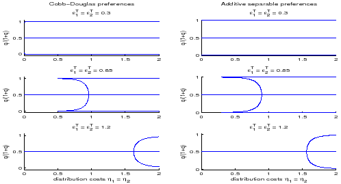
Notes: Set of normalized relative
prices ![]() that constitute a steady state absent
financial markets as a function of the distribution cost
parameters. Except for the elasticity of substitution between
traded goods and the distribution cost parameters, parameters are
chosen to match the calibration in Corsetti, Dedola, and Leduc (2008).
that constitute a steady state absent
financial markets as a function of the distribution cost
parameters. Except for the elasticity of substitution between
traded goods and the distribution cost parameters, parameters are
chosen to match the calibration in Corsetti, Dedola, and Leduc (2008).
5.2 Steady States Under Different Assumptions on International Financial Markets
The choice of the stationarity inducing device affects the
number of steady state equilibria. In a steady state with zero net
foreign assets, the standard incomplete markets model, the
portfolio cost model, and the debt-elastic interest rate model
imply the same steady state restrictions as the model without
international financial markets. If under financial autarchy
multiple values of the relative price ![]() induce market
clearing, then this is also the case for these three frameworks.
Similarly, the overlapping generations model with incomplete
markets displays the same steady states as its analogue without
financial markets.10
induce market
clearing, then this is also the case for these three frameworks.
Similarly, the overlapping generations model with incomplete
markets displays the same steady states as its analogue without
financial markets.10
By contrast, for a given parameterization of the discount factor
functions, the model with endogenous discounting admits a unique
steady state irrespective of the number of steady states under
financial autarchy. Condition (39) determines
uniquely the steady state allocations and prices including the
relative price ![]() . It is not guaranteed that the
resulting steady state coincides with any of the steady states
obtained under financial autarchy. I restrict the set discount
factor functions such that the unique steady state under endogenous
discounting coincides with one of the steady states obtained under
financial autarchy and thus features a zero net foreign asset
position.
. It is not guaranteed that the
resulting steady state coincides with any of the steady states
obtained under financial autarchy. I restrict the set discount
factor functions such that the unique steady state under endogenous
discounting coincides with one of the steady states obtained under
financial autarchy and thus features a zero net foreign asset
position.
Similarly, under complete markets, for a given initial value of
![]() , condition (40) admits only one
steady state irrespective of the number of steady states in the
model with financial autarchy. As each value of
, condition (40) admits only one
steady state irrespective of the number of steady states in the
model with financial autarchy. As each value of ![]() gives rise to a different steady state, that may not
coincide with any of those obtained under financial autarchy, I
restrict attention to those values of
gives rise to a different steady state, that may not
coincide with any of those obtained under financial autarchy, I
restrict attention to those values of ![]() , that
imply a steady state that can also be obtained under financial
autarchy.
, that
imply a steady state that can also be obtained under financial
autarchy.
6 Local Equilibrium Dynamics
Turning to the dynamics of the different models in the
neighborhood of a given deterministic steady state, the model is
(log-)linearized around this steady state. Reducing the system of
equilibrium conditions to its state variables (log deviations of
the capital stocks ![]() and
and ![]() , and the absolute deviation of the net foreign
asset position
, and the absolute deviation of the net foreign
asset position
![]() , one obtains the difference
equation:
, one obtains the difference
equation: 
with the ![]() coefficient matrices
coefficient matrices
![]() and
and ![]() and the
and the ![]() state vector
state vector
 . With
 ![]() being an invertible matrix for the models
considered in this paper, a simple count of the eigenvalues of the
matrix
being an invertible matrix for the models
considered in this paper, a simple count of the eigenvalues of the
matrix ![]() suffices to characterize the
stability of the local dynamics as described in [Christiano
2002].11 Let
suffices to characterize the
stability of the local dynamics as described in [Christiano
2002].11 Let ![]() (here equal
6) denote the number of eigenvalues of
(here equal
6) denote the number of eigenvalues of ![]() and
and
![]() be the number of eigenvalues
larger than one in absolute value.
be the number of eigenvalues
larger than one in absolute value. ![]() (here equal
to 3) is the number of predetermined variables. The equilibrium
dynamics identified by the minimum state variable solution are:
(here equal
to 3) is the number of predetermined variables. The equilibrium
dynamics identified by the minimum state variable solution are:
- bounded and unique, if
 ,
, - bounded, but not unique, if
 ,
, - unbounded, if
 .
.
Thus, the equilibrium dynamics can be characterized by the
absolute value of the ![]() th and
th and ![]() st smallest eigenvalue,
st smallest eigenvalue, ![]() and
and
![]() . If
. If
![]() , the equilibrium
dynamics are unbounded. If
, the equilibrium
dynamics are unbounded. If
![]() and
and
![]() , the dynamics
are bounded and unique. Otherwise, they are bounded, but not
unique. As
, the dynamics
are bounded and unique. Otherwise, they are bounded, but not
unique. As
![]() for all cases
analyzed below, I will reduce attention to
for all cases
analyzed below, I will reduce attention to ![]() . The subsequent analysis also links
. The subsequent analysis also links
![]() to the slope of the
excess demand function for good
to the slope of the
excess demand function for good ![]() with respect to the
relative price
with respect to the
relative price
![]() in a
steady state.
in a
steady state.
To study the relationship between the stability of the
equilibrium dynamics around a steady state and the multiplicity of
steady states, I analyze the model with endogenous capital and
traded goods (model II) as well as the model with distribution
costs (model IV) under different stationarity inducing devices. In
the following,
![]() and
and
![]() are always set to be
equal.
are always set to be
equal.
6.1 Results for Model II
Figures 4 and 5 perform this
stability analysis for model II. Figure 4 examines the
cases of standard incomplete markets, portfolio costs, and
overlapping generations. For each value of the elasticity of
substitution
![]() ,
the model is linearized around each of the steady states that exist
for
,
the model is linearized around each of the steady states that exist
for
![]() . The value of the
. The value of the
![]() th smallest eigenvalue of the system
th smallest eigenvalue of the system
![]() (left scale) and the
slope of the excess demand function for good 2 in the steady state (right scale) are recorded. In accordance with
the second panel in Figure 2, there are three
steady states for
(left scale) and the
slope of the excess demand function for good 2 in the steady state (right scale) are recorded. In accordance with
the second panel in Figure 2, there are three
steady states for
![]() in the
standard incomplete markets model and the portfolio cost model, but
a unique one otherwise. For the overlapping generations model the
value is
in the
standard incomplete markets model and the portfolio cost model, but
a unique one otherwise. For the overlapping generations model the
value is
![]() . The label
"low q steady state" refers to steady states represented by the
lower branch in Figure 2 for model II
with Cobb-Douglas preferences. "High q steady state" and "
. The label
"low q steady state" refers to steady states represented by the
lower branch in Figure 2 for model II
with Cobb-Douglas preferences. "High q steady state" and "![]() steady state" refer to the top and
middle branches, respectively.
steady state" refer to the top and
middle branches, respectively.
Under standard incomplete markets (left column) ![]() equals unity irrespective of both the
steady state around which the model is approximated and the value
of
equals unity irrespective of both the
steady state around which the model is approximated and the value
of
![]() . This finding simply
restates the non-stationarity of the net foreign asset
position.
. This finding simply
restates the non-stationarity of the net foreign asset
position.
Figure 4: Local Dynamics in Model II (BKK) Unstable Models
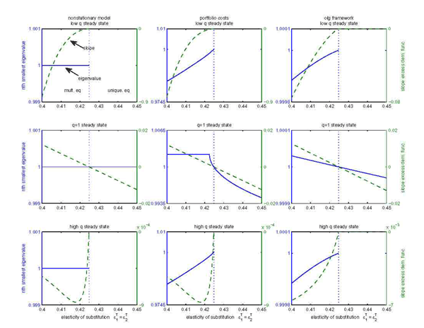
Notes: "Low q steady state" refers
to steady states represented by the lower branch in Figure 2 for model II
with Cobb-Douglas preferences. "High q steady state" and
"![]() steady state" refer to the top and
middle branch, respectively. Each panel shows the nth largest
eigenvalue (left axis) and the slope of the excess demand function
(right axis) associated with the steady state around which the
model is approximated as a function of the elasticity of
substitution between traded goods. For all three models n equals 3
and
steady state" refer to the top and
middle branch, respectively. Each panel shows the nth largest
eigenvalue (left axis) and the slope of the excess demand function
(right axis) associated with the steady state around which the
model is approximated as a function of the elasticity of
substitution between traded goods. For all three models n equals 3
and ![]() . If a steady state does not exist for a
given range of the substitution elasticity, no values are
plotted.
. If a steady state does not exist for a
given range of the substitution elasticity, no values are
plotted.
For the portfolio cost model (middle column), in the top and
bottom panels, ![]() is always
smaller than 1 and the equilibrium dynamics are
therefore locally unique and bounded. In line with Section 2, the slope of
the excess demand function is always negative for these steady
states. However, in the middle panel, that shows the results for
the symmetric steady state of the model, it is
is always
smaller than 1 and the equilibrium dynamics are
therefore locally unique and bounded. In line with Section 2, the slope of
the excess demand function is always negative for these steady
states. However, in the middle panel, that shows the results for
the symmetric steady state of the model, it is
![]() with
with
![]() for
for
![]() , and it is
, and it is
![]() with
with
![]() for
for
![]() . Hence, for
. Hence, for
![]() the equilibrium
dynamics around the symmetric steady state are not bounded.
Although not shown, the same findings apply for the case of a
debt-elastic interest rate.
the equilibrium
dynamics around the symmetric steady state are not bounded.
Although not shown, the same findings apply for the case of a
debt-elastic interest rate.
Figure 5: Local Dynamics in Model II (BKK) Stable Models
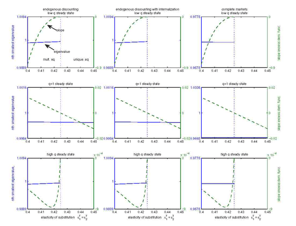
Notes: "Low q steady state" refers
to steady states represented by the lower branch in Figure 2 for model II
with Cobb-Douglas preferences. "High q steady state" and
"![]() steady state" refer to the top and
middle branch, respectively. Each panel shows the nth largest
eigenvalue (left axis) and the slope of the excess demand function
(right axis) associated with the steady state around which the
model is approximated as a function of the elasticity of
substitution between traded goods. For the first two models n
equals 3 and
steady state" refer to the top and
middle branch, respectively. Each panel shows the nth largest
eigenvalue (left axis) and the slope of the excess demand function
(right axis) associated with the steady state around which the
model is approximated as a function of the elasticity of
substitution between traded goods. For the first two models n
equals 3 and ![]() , for the complete markets model n=2
and
, for the complete markets model n=2
and ![]() . If a steady state does not exist for a
given range of the substitution elasticity, no values are
plotted.
. If a steady state does not exist for a
given range of the substitution elasticity, no values are
plotted.
In the overlapping generations framework (right column) the same
patterns arise: steady states for which the excess demand function
is downward sloping are associated with
![]() and locally unique
and bounded dynamics. Otherwise, the equilibrium dynamics are
unbounded.
and locally unique
and bounded dynamics. Otherwise, the equilibrium dynamics are
unbounded.
The local dynamics under endogenous discounting - both with and
without internalization - and under complete markets are studied in
Figure 5. As pointed out
earlier, for a given parameterization of the discount factor
function or the choice of ![]() , these three
settings always imply a unique steady state. The figure, though,
shows results for each of the steady states that occur under
financial autarchy by appropriately adjusting the discount factor
function or the weight
, these three
settings always imply a unique steady state. The figure, though,
shows results for each of the steady states that occur under
financial autarchy by appropriately adjusting the discount factor
function or the weight ![]() , respectively. The first
two columns reveal that
, respectively. The first
two columns reveal that ![]() is
always less than unity irrespective of the steady state that is
analyzed and the associated sign of
is
always less than unity irrespective of the steady state that is
analyzed and the associated sign of
![]() . Thus,
under endogenous discounting, the equilibrium dynamics are always
unique and bounded. The same findings apply under complete
markets.
. Thus,
under endogenous discounting, the equilibrium dynamics are always
unique and bounded. The same findings apply under complete
markets.
6.2 Results for Model IV
The dynamic characteristics of model IV under the calibration of Corsetti, Dedola, and Leduc (2008) with Cobb-Douglas preferences are examined in Figure 6 for the case of portfolio costs and endogenous discounting. Each of the five panels per column corresponds to one of the steady states depicted in the fourth panel of Figure 2.
For the portfolio cost model, ![]() is always less than unity in the first and fifth panels and
is always less than unity in the first and fifth panels and
![]() . To
the extent that these steady states exist, which is the case for
. To
the extent that these steady states exist, which is the case for
![]() , these steady
states are associated with unique and bounded equilibrium dynamics.
For the second and fourth panels,
, these steady
states are associated with unique and bounded equilibrium dynamics.
For the second and fourth panels, ![]() is always larger than unity and the
equilibrium dynamics are unbounded. Consistent with all previous
findings, the sign of
is always larger than unity and the
equilibrium dynamics are unbounded. Consistent with all previous
findings, the sign of
![]() is
positive. The case of
is
positive. The case of ![]() (third panel) is more
interesting. For
(third panel) is more
interesting. For
![]() ,
,
![]() is
negative and
is
negative and
![]() . It is only for
. It is only for
![]() that the excess
demand function switches sign,
that the excess
demand function switches sign, ![]() turns larger than one, and the equilibrium dynamics become
unbounded. Under endogenous discounting
turns larger than one, and the equilibrium dynamics become
unbounded. Under endogenous discounting ![]() is always smaller than one irrespective
of the steady state around which the model is approximated and the
sign of
is always smaller than one irrespective
of the steady state around which the model is approximated and the
sign of
![]() . The
equilibrium dynamics are unique and bounded.
. The
equilibrium dynamics are unique and bounded.
Figure 6: Local Dynamics in Model IV (CDL) with Cobb-Douglas Preferences
![Figure 6: The labels 'very low q steady state', 'low q steady state', 'q=1 steady state', 'high q steady state', and 'very high q steady state' refer to the steady states represented by the bottom, second from bottom, middle, second from top, and top branch in Figure 2 for model IV with Cobb-Douglas preferences, respectively. Each panel shows the nth largest eigenvalue (left axis) and the slope of the excess demand function (right axis) associated with the steady state around which the model is approximated as a function of the elasticity of substitution between traded goods. For both models n equals 3 and N=6. If a steady state does not exist for a given range of the substitution elasticity, no values are plotted. The steady state is unique for varepsilon^T_{1}>0.9798. There are five steady states for varepsilon^T_{1} in [0.9189;0.9798] and three steady states for varepsilon^T_{1}<0.9189.](img471.gif)
Notes: The labels "very low q steady
state", "low q steady state", "![]() steady
state", "high q steady state", and "very high q steady state"
refer to the steady states represented by the bottom, second from
bottom, middle, second from top, and top branch in Figure 2 for model IV
with Cobb-Douglas preferences, respectively. Each panel shows the
nth largest eigenvalue (left axis) and the slope of the excess
demand function (right axis) associated with the steady state
around which the model is approximated as a function of the
elasticity of substitution between traded goods. For both models n
equals 3 and
steady
state", "high q steady state", and "very high q steady state"
refer to the steady states represented by the bottom, second from
bottom, middle, second from top, and top branch in Figure 2 for model IV
with Cobb-Douglas preferences, respectively. Each panel shows the
nth largest eigenvalue (left axis) and the slope of the excess
demand function (right axis) associated with the steady state
around which the model is approximated as a function of the
elasticity of substitution between traded goods. For both models n
equals 3 and ![]() . If a steady state does not exist for
a given range of the substitution elasticity, no values are
plotted. The steady state is unique for
. If a steady state does not exist for
a given range of the substitution elasticity, no values are
plotted. The steady state is unique for
![]() . There are five
steady states for
. There are five
steady states for
![]() and
three steady states for
and
three steady states for
![]() .
.
Figure 7: Local Dynamics in Model IV (CDL) with Additit
![Figure 7: The labels 'very low q steady state', 'low q steady state', 'q=1 steady state', 'high q steady state', and 'very high q steady state' refer to the steady states represented by the bottom, second from bottom, middle, second from top, and top branch in Figure 2 for model IV with additive separable preferences, respectively. Each panel shows the nth largest eigenvalue (left axis) and the slope of the excess demand function (right axis) associated with the steady state around which the model is approximated as a function of the elasticity of substitution between traded goods. For both models n equals 3 and N=6. If a steady state does not exist for a given range of the substitution elasticity, no values are plotted. The steady state is unique for varepsilon^T_{1}>1.0115. There are five steady states for varepsilon^T_{1} in [0.9516;1.0115] and three steady states for varepsilon^T_{1}<0.9516.](img477.gif)
Notes: The labels "very low q steady
state", "low q steady state", "![]() steady
state", "high q steady state", and "very high q steady state"
refer to the steady states represented by the bottom, second from
bottom, middle, second from top, and top branch in Figure 2 for model IV
with additive separable preferences, respectively. Each panel shows
the nth largest eigenvalue (left axis) and the slope of the excess
demand function (right axis) associated with the steady state
around which the model is approximated as a function of the
elasticity of substitution between traded goods. For both models n
equals 3 and
steady
state", "high q steady state", and "very high q steady state"
refer to the steady states represented by the bottom, second from
bottom, middle, second from top, and top branch in Figure 2 for model IV
with additive separable preferences, respectively. Each panel shows
the nth largest eigenvalue (left axis) and the slope of the excess
demand function (right axis) associated with the steady state
around which the model is approximated as a function of the
elasticity of substitution between traded goods. For both models n
equals 3 and ![]() . If a steady state does not exist for
a given range of the substitution elasticity, no values are
plotted. The steady state is unique for
. If a steady state does not exist for
a given range of the substitution elasticity, no values are
plotted. The steady state is unique for
![]() and
three steady states for
and
three steady states for
![]() .
.
Figure 8: Local Dynamics in Model IV (CDL) with Additive Separable Preferences, Real and Nominal Rigidities
![Figure 8: The labels 'very low q steady state', 'low q steady state', 'q=1 steady state', 'high q steady state', and 'very high q steady state' refer to the steady states represented by the bottom, second from bottom, middle, second from top, and top branch in Figure ref{bifurcationplots_changesepsilon_all} for model IV with additive separable preferences, respectively. Panels show the nth largest eigenvalue (left axis) and the slope of the excess demand function (right axis) associated with the steady state around which the model is approximated as a function of the elasticity of substitution between traded goods. Due to the additional state variables n equals 40 and N=78. The steady state is unique for varepsilon^T_{1}>1.0115. There are five steady states for varepsilon^T_{1} in [0.9516;1.0115] and three steady states for varepsilon^T_{1}<0.9516. Monetary policy follows a Taylor-type rule with a long-run weight on consumer price inflation of 1.5, an interest rate smoothing coefficient of 0.7, and zero weight on the output gap.](img483.gif)
Notes: The labels "very low q steady
state", "low q steady state", "![]() steady
state", "high q steady state", and "very high q steady state"
refer to the steady states represented by the bottom, second from
bottom, middle, second from top, and top branch in Figure 2 for model IV
with additive separable preferences, respectively. Panels show the
nth largest eigenvalue (left axis) and the slope of the excess
demand function (right axis) associated with the steady state
around which the model is approximated as a function of the
elasticity of substitution between traded goods. Due to the
additional state variables n equals 40 and
steady
state", "high q steady state", and "very high q steady state"
refer to the steady states represented by the bottom, second from
bottom, middle, second from top, and top branch in Figure 2 for model IV
with additive separable preferences, respectively. Panels show the
nth largest eigenvalue (left axis) and the slope of the excess
demand function (right axis) associated with the steady state
around which the model is approximated as a function of the
elasticity of substitution between traded goods. Due to the
additional state variables n equals 40 and ![]() . The
steady state is unique for
. The
steady state is unique for
![]() . There are five
steady states for
. There are five
steady states for
![]() and
three steady states for
and
three steady states for
![]() . Monetary policy
follows a Taylor-type rule with a long-run weight on consumer price
inflation of 1.5, an interest rate smoothing coefficient of 0.7,
and zero weight on the output gap.
. Monetary policy
follows a Taylor-type rule with a long-run weight on consumer price
inflation of 1.5, an interest rate smoothing coefficient of 0.7,
and zero weight on the output gap.
Allowing for additive separable preferences does not overturn these findings as shown in Figure 7. Introducing real and nominal rigidities under additive separable preferences does not affect the findings either. Figure 8 confirms this claim in a model with Calvo sticky wage and price contracts, consumption habits, investment adjustment costs, and local currency pricing. Monetary policy follows an interest rate rule with the policy rate being a function of consumer price inflation only. A detailed model description is provided in the Technical Appendix accompanying this paper.
7 Conclusions
Widely used international business cycle models admit multiple steady states absent international financial markets for low substitutability between traded goods. Once a limited set of internationally traded assets is introduced, the steady state multiplicity may or may not be preserved. If the incomplete markets model is augmented with portfolio costs, a debt-elastic interest rate, or an overlapping generations framework as in Weil (1989) the number of steady states remains unchanged relative to the model without financial markets. If Uzawa-type preferences are introduced (Uzawa (1968)), the steady state of the model is unique.
The choice of stationarity inducing device also affects the stability of the dynamics around a given steady state. Under portfolio costs, debt-elastic interest rates, or overlapping generations, steady states that are associated with a downward-sloping excess demand function of the foreign good display locally unique and bounded dynamics. For steady states with an upward-sloping excess demand function, the local dynamics are unbounded. Under endogenous discounting or complete markets, the local dynamics are always unique and bounded.
The results stressed in this paper prevail under (local) higher order perturbation methods. The findings also extend to environments with a larger set of available assets. If country portfolios are determined as in Devereux and Sutherland (2008) and Tille and van Wincoop (2010), the net foreign asset position is not determined in steady state and displays unit root behavior unless stationarity is induced with one of the devices discussed in this paper.
Absent trade adjustment costs short- and long-run substitution
elasticities are identical in this paper. If trade adjustment costs
were to affect the model's allocations away from a steady state,
the analysis would not change given the use of local solution
techniques. Steady state multiplicity would only occur if the
long-run substitution elasticity between traded goods fell below
its threshold level
![]() in the model
without trade adjustment costs. However, if one were to employ
global solution techniques, differences across models could be
detected. Similar to the findings presented in Bodenstein (2010)
for the case of capital, a lower short-run substitution elasticity
may lead to multiple equilibrium paths despite a unique steady
state for the given value of the long-run substitution
elasticity.
in the model
without trade adjustment costs. However, if one were to employ
global solution techniques, differences across models could be
detected. Similar to the findings presented in Bodenstein (2010)
for the case of capital, a lower short-run substitution elasticity
may lead to multiple equilibrium paths despite a unique steady
state for the given value of the long-run substitution
elasticity.
Bibliography
Backus, D., P. Kehoe, and F. Kydland (1995). International business cycles: theory and evidence. In T. Cooley (Ed.), Frontiers of Business Cycle Research, pp. 331-356. Princeton University Press.
Backus, D. K. and G. W. Smith (1993). Consumption and real exchange rates in dynamic exchange economies with non-traded goods. Journal of International Economics 35(3-4), 297-316.
Baxter, M. and M. J. Crucini (1995). Business cycles and the asset structure of foreign trade. International Economic Review 36(4), 821-54.
Benigno, G. and C. Thoenissen (2008). Consumption and real exchange rates with incomplete markets and non-traded goods. Journal of International Money and Finance 27(6), 926-948.
Bodenstein, M. (2010). Trade elasticity of substitution and equilibrium dynamics. Journal of Economic Theory 145(3), 1033-1059.
Boileau, M. and M. Normandin (2008). Closing international real business cycle models with restricted financial markets. Journal of International Money and Finance 27(5), 733-756.
Broda, C. and D. E. Weinstein (2006). Globalization and the gains from variety. The Quarterly Journal of Economics 121(2), 541-585.
Burstein, A. T., J. C. Neves, and S. Rebelo (2003). Distribution costs and real exchange rate dynamics during exchange-rate-based stabilizations. Journal of Monetary Economics 50(6), 1189-1214.
Chari, V. V., P. J. Kehoe, and E. R. McGrattan (2002). Can sticky price models generate volatile and persistent real exchange rates? Review of Economic Studies 69(3), 533-63.
Christiano, L. J. (2002). Solving dynamic equilibrium models by a method of undetermined coefficients. Computational Economics 20(1-2), 21-55.
Collard, F. and H. Dellas (2007). Technology shocks and employment. Economic Journal 117(523), 1436-1459.
Corsetti, G. and L. Dedola (2005). A macroeconomic model of international price discrimination. Journal of International Economics 67(1), 129-155.
Corsetti, G., L. Dedola, and S. Leduc (2008). International risk sharing and the transmission of productivity shocks. Review of Economic Studies 75(2), 443-473.
Devereux, M. B. and G. W. Smith (2007). Transfer problem dynamics: macroeconomics of the franco-prussian war indemnity. Journal of Monetary Economics 54(8), 2375-2398.
Devereux, M. B. and A. Sutherland (2008). Financial globalization and monetary policy. Journal of Monetary Economics 55(8), 1363-1375.
Ghironi, F. (2006). Macroeconomic interdependence under incomplete markets. Journal of International Economics 70(2), 428-450.
Ghironi, F. (2008). The role of net foreign assets in a new keynesian small open economy model. Journal of Economic Dynamics and Control 32(6), 1780-1811.
Heathcote, J. and F. Perri (2002). Financial autarky and international business cycles. Journal of Monetary Economics 49(3), 601-627.
Hooper, P., K. Johnson, and J. Marquez (1998). Trade elasticities for g-7 countries. International Finance Discussion Papers 609, Board of Governors of the Federal Reserve System (U.S.).
Kehoe, T. J. (1991). Computation and multiplicity of equilibria. In W. Hildenbrand and H. Sonnenschein (Eds.), Handbook of Mathematical Economics, Volume 4 of Handbook of Mathematical Economics, Chapter 38, pp. 2049-2144. Elsevier.
Kim, S. and M. Kose (2003). Dynamics of open-economy business-cycle models: role of the discount factor. Macroeconomic Dynamics 7(2), 263-290.
Kollmann, R. (2006, February). International portfolio equilibrium and the current account. CEPR Discussion Papers 5512, C.E.P.R. Discussion Papers.
Lubik, T. and F. Schorfheide (2006). A bayesian look at the new open economy macroeconomics. In NBER Macroeconomics Annual 2005, Volume 20, NBER Chapters, pp. 313-382. National Bureau of Economic Research, Inc.
Mas-Colell, A., M. Whinston, and J. Green (1995). Microeconomic Theory. Oxford University Press.
Mendoza, E. G. (1991). Real business cycles in a small open economy. American Economic Review 81(4), 797-818.
Rabanal, P. and V. Tuesta (2010). Euro-dollar real exchange rate dynamics in an estimated two-country model: An assessment. Journal of Economic Dynamics and Control 34(4), 780-797.
Schmitt-Grohé, S. and M. Uribe (2003). Closing small open economy models. Journal of International Economics 61(1), 163-185.
Stockman, A. C. and L. L. Tesar (1995). Tastes and technology in a two-country model of the business cycle: explaining international comovements. American Economic Review 85(1), 168-85.
Taylor, J. (1993). Macroeconomic policy in a world economy: from economic design to practical operation. Norton, New York, NY.
Tille, C. and E. van Wincoop (2010). International capital flows. Journal of International Economics 80(2), 157-175.
Uzawa, H. (1968). Value, capital and growth: papers in honor of sir john hicks. In J. Wolfe (Ed.), Time preference, the consumption function and optimum asset holdings, pp. 485-504. The University of Edinburgh Press.
Weil, P. (1989). Overlapping families of infinitely-lived agents. Journal of Public Economics 38(2), 183-198.
Whalley, J. (1984, June). Trade Liberalization among Major World Trading Areas, Volume 1 of MIT Press Books. The MIT Press.
A Appendix: Details on the Simple Model
This appendix describes the equations underlying the discussion in Section 2. The first order conditions of the households imply:
![$\displaystyle c_{12,t} =\frac{\alpha _{12}^T q_t ^{-\varepsilon^T }}{\alpha _{11}^T +\alpha _{12}^T q_t^{1-\varepsilon^T }}\left[ y^T_{1,t} +\frac{b_{1,t-1} -Q_{1,t} b_{1,t} }{\Phi_1(q_{t})}\right] ,$](img490.gif) |
(50) |
![$\displaystyle c_{22,t} =\frac{\alpha _{22}^T }{\alpha _{21}^T \left( \frac{1}{ q_t}\right) ^{1-\varepsilon^T }+\alpha _{22}^T }\left[ y^T_{2,t} +\frac{b_{2,t-1} -Q_{2,t} b_{2,t}}{\Phi_1(q_t) q_t}\right],$](img491.gif) |
(51) |
| (52) | |
 |
(53) |
where
![$\displaystyle \frac{P_{1,t}}{P_{1,t}c_{11,t}+P_{2,t}c_{12,t}} = \left[ \alpha^T _{11}\left( \frac{1}{ q_t }\right) ^{1-\varepsilon^T }+\alpha^T _{12}\right] ^{- \frac{1}{1-\varepsilon^T }}\frac{1}{q_t }\text{ },$](img496.gif) |
(54) |
![$\displaystyle \frac{P_{2,t}}{P_{1,t}c_{21,t}+P_{2,t}c_{22,t}} =\left[ \alpha^T _{21}\left( \frac{1}{ q_t }\right) ^{1-\varepsilon^T }+\alpha^T _{22}\right] ^{- \frac{1}{1-\varepsilon^T }}\text{ },$](img499.gif) |
(55) |
 |
(56) |
The price of the aggregate consumption good in country 1 is taken to be the numéraire. Log-linearizing these
equations around a steady state with zero net foreign assets and
setting the exogenous variables ![]() and
and
![]() to be constant ("
to be constant ("![]() " for log-linearized and "
" for log-linearized and "![]() " for
linearized variables
" for
linearized variables ![]() ). Variables without time
index indicate steady state values:
). Variables without time
index indicate steady state values:
![$\displaystyle -\left\{ (1-\varepsilon^T)(1-\alpha^T_{11})+\varepsilon^T \right\} \hat{q}_{t} +\frac{1}{y_{1}\Phi _{1}(q) }\left[ \Delta b_{1,t-1}-\beta \Delta b_{1,t}\right] ,$](img511.gif) |
(57) |
![$\displaystyle (1-\varepsilon^T)(1-{\alpha}^T_{22}) \hat{q}_{t} -\frac{1}{q\Phi _{1}(q) y_{2}}\left[ \Delta b_{1,t-1}-\beta \Delta b_{1,t}\right],$](img514.gif) |
(58) |
| (59) |
where I have used the fact that in steady state
![]() and
and
![]() .
.
Using (57) and (58) in the approximation of the market clearing condition for good 2:
![$\displaystyle \frac{\partial z_{2}}{\partial q}q \hat{q}_{t} +\frac{\partial z_{2}}{\partial dW_{1}} \left[ \Delta b_{1t-1}-\beta \Delta b_{1t} \right] = 0,$](img521.gif) |
(60) |
with the coefficients
 |
(61) |
  |
(62) |
Note that in a steady state with balanced trade
![]() . The
slope of the excess demand function in steady state with respect to
. The
slope of the excess demand function in steady state with respect to
![]() is given by equation (61).
is given by equation (61).
Aggregate consumption is determined by:
 |
(63) |
 |
(64) |
while the risk sharing condition is given by:
|
(65) |
Thus, the dynamic system under portfolio costs can be written as:
 |
(66) |
with the coefficients
|
(67) |
![$\displaystyle \frac{\gamma}{\beta ^{2}\Phi _{1}(q) }\left[ 1+\frac{1}{q}\right]>0.$](img545.gif)
|
(68) |
Hence, the characteristic equation associated with the dynamic system (66) under the portfolio cost approach satisfies:
 |
(69) |
Alternatively, assume that households have Uzawa-type preferences.
The time discount factor ![]() is replaced by
is replaced by
![]() with
with
![]() .
. ![]() is chosen such that
is chosen such that
![]() in steady state.
Absent internalization, the risk sharing condition implies:
in steady state.
Absent internalization, the risk sharing condition implies:
| (70) |
Hence, the characteristic equation associated with the dynamic system under endogenous discounting without internalization satisfies:
 |
(71) |
with
![\begin{displaymath} \widetilde{dz_2}=-\frac{1}{q\Phi _{1}\left( q\right) }\left[ \frac{\beta _{1}^{\prime }(q) }{\beta _{1}(q)}\left( 1-\frac{c_{21}(q)}{y_{1}^{T}}\right) +\frac{\beta _{2}^{\prime }(q)}{\beta _{2}(q)}\left( 1-\frac{c_{22}(q)}{y_{2}^{T}}\right) \right] {\normalsize\varepsilon ^{T}\left\{ \frac{c_{11}(q)}{y_{1}^{T}}+\frac{c_{22}(q)}{ y_{2}^{T}}\right\}>0,} \end{displaymath}](img554.gif) |
(72) |
as the discount factors are assumed to be decreasing in the level
of consumption.12
B Appendix: Overlapping Generations Model
This appendix merges the framework with overlapping generations of infinitely lived households by Weil (1989) and Ghironi (2006) with the model presented in the main text. Absent Ricardian equivalence, the steady state level of the net foreign asset position can be shown to be unique. Furthermore, the local dynamics of the net foreign asset position are stationary. More details on the overlapping generations framework are provided in the Technical Appendix accompanying this paper.
Each household consumes, supplies labor, and holds financial
assets. Households are born on different dates owning no assets,
but they own the present discounted value of their labor income.
The number of households in country ![]()
![]() grows over time at the exogenous rate
grows over time at the exogenous rate ![]() , i.e.,
, i.e.,
![]() . The
utility function of each household is assumed to be of the
Cobb-Douglas type. Capital is no longer accumulated by households
directly, but through capital producers. Households can purchase
shares in these and all other firms that produce in their country
of residence.
. The
utility function of each household is assumed to be of the
Cobb-Douglas type. Capital is no longer accumulated by households
directly, but through capital producers. Households can purchase
shares in these and all other firms that produce in their country
of residence.
B.1 Individual Households
Consumers have identical preferences over the real consumption
index and leisure. At time ![]() , the
representative consumer in country
, the
representative consumer in country ![]() born in
period
born in
period
![]() maximizes
the intertemporal utility function:
maximizes
the intertemporal utility function:
|
(73) |
| (74) |
The final consumption of a representative household of country
![]() born in period
born in period ![]() at time
at time
![]() is denoted by
is denoted by ![]() .
The production of the final consumption good follows the same
process as outlined in the main text.
.
The production of the final consumption good follows the same
process as outlined in the main text. ![]() is
the labor supply of such a household. The bond holdings are denoted
by
is
the labor supply of such a household. The bond holdings are denoted
by ![]() .
.
![]() are the household's holdings
of the domestic stock, that sells at the price
are the household's holdings
of the domestic stock, that sells at the price
![]() and pays the dividend
and pays the dividend
![]() . The supply of the stock is
normalized to 1.
. The supply of the stock is
normalized to 1.
B.2 Firms
While I assume that the production structure of the economy is unchanged relative to the main text, capital is held by capital producers. These firms buy the investment good, augment the existing capital stock, and rent out capital to the producers of traded and non-traded goods. They also pay a dividend to the stockholders. The optimization problem of the capital producers is given by:
|
(75) |
![]() is the pricing kernel used
by the capital producers to discount future profits. The capital
used in time
is the pricing kernel used
by the capital producers to discount future profits. The capital
used in time ![]() production,
production, ![]() , and
investment,
, and
investment, ![]() , are expressed as per capita
averages. The average per capital dividend payment is denoted by
, are expressed as per capita
averages. The average per capital dividend payment is denoted by
![]() and satisfies
and satisfies
![]() .
.
Footnotes
* I have benefited from conversations with Roc Armenter, Fabio Ghironi, Sylvain Leduc, and Thomas Lubik. I am particularly grateful to two anonymous referees and Giancarlo Corsetti (the editor) whose suggestions have substantially improved the paper. All remaining errors are mine. The views expressed in this paper are solely the responsibility of the author and should not be interpreted as reflecting the views of the Board of Governors of the Federal Reserve System or any other person associated with the Federal Reserve System. Return to text
*** Contact information: Martin Bodenstein: phone (202) 452 3796, [email protected]. Return to text
1. Prominent examples of such models are found in Backus, Kehoe, and Kydland (1995), Baxter and Crucini (1995), Heathcote and Perri (2002), and Stockman and Tesar (1995). However, none of these papers explores the possibility of multiple steady states, as the elasticity of substitution is generally assumed to be above unity. Return to text
2. In the working paper version of Corsetti and Dedola (2005), the authors point out that for the case of an endowment economy a model with distribution costs admits multiple equilibria in the absence of international borrowing and lending. However, no systematic exploration of this feature is conducted. Return to text
3. Multiplicity of the steady state price vector can also occur if the net foreign asset position differs from zero in steady state. However, the assumption of zero net foreign assets in steady state is widely made in the literature and implies that the steady states of the incomplete markets model coincide with those obtained in a model without financial markets. Return to text
4. While throughout the analysis the only asset that trades internationally is one non-state-contingent bond, the issues raised carry over to environments with more assets such as those presented in Devereux and Sutherland (2008) as long as the available assets do not complete the market. Return to text
5. If the discount factor was increasing in the agent's utility level, the dynamics around any steady state would always be unbounded. Return to text
6. Corsetti, Dedola, and Leduc (2008) argue that a positive supply shock to the home country can cause an appreciation of the home country's terms of trade when the excess demand function is upward sloping in the steady state around which the model is linearized. Absent "the negative transmission mechanism" their model can resolve the Backus-Smith puzzle only for very persistent shock processes. Return to text
7. The net foreign asset position
becomes non-stationary as a result of using local solution
techniques. While higher order perturbation methods imply the same
problems as a linear solution approach, global solution methods do
not. If the model was solved using global methods, stationarity
would be preserved due to the presence of the borrowing constraints
![]() . In addition, the concept of a
deterministic steady state would need to be replaced by that of a
stationary distribution. Return to
text
. In addition, the concept of a
deterministic steady state would need to be replaced by that of a
stationary distribution. Return to
text
8.
![]() is the absolute deviation of
real bond holdings
is the absolute deviation of
real bond holdings
![]() from zero. Return to text
from zero. Return to text
9. Numerically, the steady state value of
the prices of the non-traded goods do not vary with
![]() . While in equation
(32) the
measured trade elasticity in the symmetric steady state is
proportional to the elasticity of substitution between traded
goods, this is not true for the asymmetric steady
states. Return to text
. While in equation
(32) the
measured trade elasticity in the symmetric steady state is
proportional to the elasticity of substitution between traded
goods, this is not true for the asymmetric steady
states. Return to text
10. As shown in Appendix B, the steady states in the overlapping generations model differ from the steady states in models for which each country's agents can be represented by a single agent. However, for the parameterizations adopted in this paper, the quantitative differences are small. Return to text
11. [Christiano 2002] discusses also the
case if ![]() is not invertible. Return to text
is not invertible. Return to text
12. If the discount factors were
increasing in the level of consumption,
![]() would be negative and the
dynamics around any deterministic steady state would be
explosive. Return to text
would be negative and the
dynamics around any deterministic steady state would be
explosive. Return to text
Closing Large Open Economy Models: Technical Appendix
Abstract:
This Technical Appendix describes the details of the following topics in the paper "Closing large open economy models:" the simple example of Section 2, the linearized model equations of the model in the main text, the overlapping generations framework, and the model with real and nominal rigidities.
A Appendix: Details on the Simple Model
This appendix describes the equations underlying the discussion in Section 2. The first order conditions of the households imply:
![$\displaystyle c_{12,t} =\frac{\alpha _{12}^T q_t ^{-\varepsilon^T }}{\alpha _{11}^T +\alpha _{12}^T q_t^{1-\varepsilon^T }}\left[ y^T_{1,t} +\frac{b_{1,t-1} -Q_{1,t} b_{1,t} }{\Phi_1(q_{t})}\right] ,$](img2t.gif) |
(1) |
![$\displaystyle c_{22,t} =\frac{\alpha _{22}^T }{\alpha _{21}^T \left( \frac{1}{ q_t}\right) ^{1-\varepsilon^T }+\alpha _{22}^T }\left[ y^T_{2,t} +\frac{b_{2,t-1} -Q_{2,t} b_{2,t}}{\Phi_1(q_t) q_t}\right],$](img3t.gif) |
(2) |
| (3) | |
 |
(4) |
where
![$\displaystyle \frac{P_{1,t}}{P_{1,t}c_{11,t}+P_{2,t}c_{12,t}} = \left[ \alpha^T _{11}\left( \frac{1}{ q_t }\right) ^{1-\varepsilon^T }+\alpha^T _{12}\right] ^{- \frac{1}{1-\varepsilon^T }}\frac{1}{q_t }\text{ },$](img8t.gif) |
(5) |
![$\displaystyle \frac{P_{2,t}}{P_{1,t}c_{21,t}+P_{2,t}c_{22,t}} =\left[ \alpha^T _{21}\left( \frac{1}{ q_t }\right) ^{1-\varepsilon^T }+\alpha^T _{22}\right] ^{- \frac{1}{1-\varepsilon^T }}\text{ },$](img11t.gif) |
(6) |
 |
(7) |
The price of the aggregate consumption good in country 1 is taken to be the numéraire. Log-linearizing these
equations around a steady state with zero net foreign assets and
setting the exogenous variables ![]() and
and ![]() to be constant ("
to be constant ("![]() " for log-linearized and "
" for log-linearized and "![]() " for
linearized variables
" for
linearized variables ![]() ). Variables without time
index indicate steady state values:
). Variables without time
index indicate steady state values:
![$\displaystyle -\left\{ (1-\varepsilon^T)(1-\alpha^T_{11})+\varepsilon^T \right\} \hat{q}_{t} +\frac{1}{y_{1}\Phi _{1}(q) }\left[ \Delta b_{1,t-1}-\beta \Delta b_{1,t}\right] ,$](img23t.gif) |
(8) |
![$\displaystyle (1-\varepsilon^T)(1-{\alpha}^T_{22}) \hat{q}_{t} -\frac{1}{q\Phi _{1}(q) y_{2}}\left[ \Delta b_{1,t-1}-\beta \Delta b_{1,t}\right],$](img26t.gif) |
(9) |
| (10) |
where I have used the fact that in steady state
![]() and
and
![]() .
.
Using (8) and (9) in the approximation of the market clearing condition for good 2:
![$\displaystyle \frac{\partial z_{2}}{\partial q}q \hat{q}_{t} +\frac{\partial z_{2}}{\partial dW_{1}} \left[ \Delta b_{1t-1}-\beta \Delta b_{1t} \right] = 0,$](img33t.gif) |
(11) |
with the coefficients
 |
(12) |
  |
(13) |
Note that in a steady state with balanced trade
![]() . The
slope of the excess demand function in steady state with respect to
. The
slope of the excess demand function in steady state with respect to ![]() is given by equation (12).
is given by equation (12).
Aggregate consumption is determined by:
 |
(14) |
 |
(15) |
while the risk sharing condition is given by:
|
(16) |
Thus, the dynamic system under portfolio costs can be written as:
 |
(17) |
with the coefficients
|
(18) |
![$\displaystyle \frac{\gamma}{\beta ^{2}\Phi _{1}(q) }\left[ 1+\frac{1}{q}\right]>0.$](img57t.gif) |
(19) |
Hence, the characteristic equation associated with the dynamic system (17) under the portfolio cost approach satisfies:
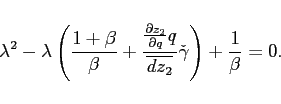 |
(20) |
Alternatively, assume that households have Uzawa-type preferences.
The time discount factor ![]() is replaced by
is replaced by
![]() with
with
![]() .
. ![]() is chosen such that
is chosen such that
![]() in steady state. Absent
internalization, the risk sharing condition implies:
in steady state. Absent
internalization, the risk sharing condition implies:
| (21) |
Hence, the characteristic equation associated with the dynamic system under endogenous discounting without internalization satisfies:
 |
(22) |
with
![\begin{displaymath} \widetilde{dz_2}=-\frac{1}{q\Phi _{1}\left( q\right) }\left[ \frac{\beta _{1}^{\prime }(q) }{\beta _{1}(q)}\left( 1-\frac{c_{21}(q)}{y_{1}^{T}}\right) +\frac{\beta _{2}^{\prime }(q)}{\beta _{2}(q)}\left( 1-\frac{c_{22}(q)}{y_{2}^{T}}\right) \right] {\normalsize\varepsilon ^{T}\left\{ \frac{c_{11}(q)}{y_{1}^{T}}+\frac{c_{22}(q)}{ y_{2}^{T}}\right\}>0,} \end{displaymath}](img66t.gif) |
(23) |
as the discount factors are assumed to be decreasing in the level of consumption.1
B Appendix: Linearized Model
This appendix describes the nonlinear first order conditions
together with their linear approximations. ![]() denotes the log-linear approximation of variable
denotes the log-linear approximation of variable ![]() from its steady state value,
from its steady state value, ![]() denotes its
deviation in absolute value:
denotes its
deviation in absolute value:
- choice of leisure in country
 :
:
- with additive separable preferences
is approximated by


- with Cobb-Douglas preferences
is approximated by


- with additive separable preferences
- choice of capital in country
 :
:
- with additive separable preferences
is approximated by
![\begin{eqnarray*} && \beta \left( \frac{c_{i,t+1}}{c_{i,t}}\right) ^{-\sigma }\frac{\Phi _{i,t+1}}{\Phi _{i,t}}\frac{\Pi _{i,t}}{\Pi _{i,t+1}}\left[ \Pi _{i,t+1}r_{i,t+1}+\left( 1-\delta \right) \right] = 1 \end{eqnarray*}](img77t.gif) which is augmented by
which is augmented by![\begin{eqnarray*} && \beta \Pi _{i}r_{i}\left[ \hat{\Pi}_{i,t+1}+\hat{r}_{i,t+1}\right] -\sigma \left( \hat{c}_{i,t+1}-\hat{c}_{i,t}\right) \ &&+\left( \hat{\Phi}_{i,t+1}-\hat{\Phi}_{i,t}\right) -\left( \hat{\Pi} _{i,t+1}-\hat{\Pi}_{i,t}\right) = 0 \end{eqnarray*}](img78t.gif)
 on the left side under
endogenous discounting
 - with Cobb-Douglas preferences
is approximated by
![\begin{eqnarray*} && \beta \left( \frac{ c_{i,t+1}^{\xi }\left( 1-l_{i,t+1}\right) ^{1-\xi }} { c_{i,t}^{\xi }\left(1-l_{i,t}\right) ^{1-\xi }} \right)^{1-\sigma }\frac{c_{i,t}}{c_{i,t+1}} \frac{\Phi _{i,t+1}}{\Phi _{i,t}}\frac{\Pi _{i,t}}{\Pi _{i,t+1}}\left[ \Pi _{i,t+1}r_{i,t+1}+\left( 1-\delta \right) \right] =1 \end{eqnarray*}](img80t.gif) which is augmented by
which is augmented by
 on the left side under
endogenous discounting
- with additive separable preferences
- capital accumulation in country
 :
is approximated by

- consumer budget constraint
- for country 1:
is approximated by


- for country 2:
is approximated by


- for country 1:
- risk sharing condition with additive separable preferences
- with adjustment costs:
under additive separable preferences is approximated by


- with debt-elastic interest rate:
is approximated by
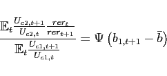

- with endogenous discounting, but no internalization
under additive separable preferences is approximated by


- with endogenous discounting and internalization:
is approximated by
 and
and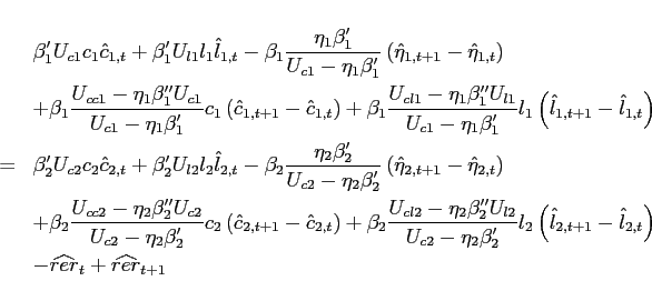

- with adjustment costs:
- endogenous discount factors
- with additive separable preferences:
is approximated by

![\begin{eqnarray*} \hat{\beta}_{i,t} &=&\frac{\beta -1}{\beta }\left[ c_{i}^{1-\sigma _{i}}\hat{ c}_{i,t}-\chi _{0}l_{i}^{1+\chi _{i}}\hat{l}_{i,t}\right] \end{eqnarray*}](img103t.gif)
- with Cobb Douglas preferences
is approximated by
![\begin{eqnarray*} \beta _{i,t} &=&\left( 1+\psi \left[ c_{i,t}^{\xi }\left( 1-l_{i,t}\right) ^{1-\xi }\right] \right) ^{-1} \end{eqnarray*}](img104t.gif)

- with additive separable preferences:
- wealth evolution
where

 implies the
approximation

- investment aggregate for country
 is approximated by
![\begin{eqnarray*} x_{i,t}&=&\left[ \left( \alpha _{i1}^{I}\right) ^{\frac{1}{\varepsilon_{i} ^{I}} }\left( x_{i1,t}\right) ^{\frac{\varepsilon_{i} ^{I}-1}{\varepsilon_{i} ^{I}} }+\left( \alpha _{i2}^{I}\right) ^{\frac{1}{\varepsilon_{i} ^{I}}}\left( x_{i2,t}\right) ^{\frac{\varepsilon_{i} ^{I}-1}{\varepsilon_{i} ^{I}}}\right] ^{ \frac{\varepsilon_{i} ^{I}}{\varepsilon_{i} ^{I}-1}} \end{eqnarray*}](img110t.gif)

- investment optimal choices
- for country 1:
is approximated by


- for country 2:
is approximated by
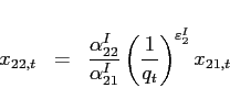

- for country 1:
- consumption aggregate over traded goods for country
 :
is approximated by
:
is approximated by![\begin{eqnarray*} c_{i,t}^{T}&=&\left[ \left( \alpha _{i1}^{T}\right) ^{\frac{1}{\varepsilon_{i} ^{T}}}\left( c_{i1,t}\right) ^{\frac{\varepsilon_{i} ^{T}-1}{\varepsilon_{i} ^{T}} }+\left( \alpha _{i2}^{T}\right) ^{\frac{1}{\varepsilon_{i} ^{T}}}\left( c_{i2,t}\right) ^{\frac{\varepsilon_{i} ^{T}-1}{\varepsilon_{i} ^{T}}}\right] ^{ \frac{\varepsilon_{i} ^{T}}{\varepsilon_{i} ^{T}-1}} \end{eqnarray*}](img119t.gif)

- consumption aggregate over traded and non traded goods for
country
 is approximated by
![\begin{eqnarray*} c_{i,t}&=&\left[ \left( \alpha _{i1}^{N}\right) ^{\frac{1}{\varepsilon_{i} ^{N}} }\left( c_{i,t}^{T}\right) ^{\frac{\varepsilon_{i} ^{N}-1}{\varepsilon_{i} ^{N}} }+\left( \alpha _{i2}^{N}\right) ^{\frac{1}{\varepsilon_{i} ^{N}}}\left( c_{i,t}^{N}\right) ^{\frac{\varepsilon_{i} ^{N}-1}{\varepsilon_{i} ^{N}}}\right] ^{ \frac{\varepsilon_{i} ^{N}}{\varepsilon_{i} ^{N}-1}} \end{eqnarray*}](img122t.gif)

- consumption optimal choices non-traded goods
- for country 1:
is approximated by
![\begin{eqnarray*} c_{1,t}^{N}&=&c_{12,t}\frac{\alpha _{12}^{N}}{\alpha _{11}^{N}}\left[ \left( \alpha _{11}^{T}\right) ^{\frac{1}{\varepsilon_{1} ^{T}}}\left( \frac{ c_{11,t}}{c_{12,t}}\right) ^{\frac{\varepsilon_{1} ^{T}-1}{\varepsilon_{1} ^{T}} }+\left( \alpha _{12}^{T}\right) ^{\frac{1}{\varepsilon_{1} ^{T}}}\right] ^{ \frac{\varepsilon_{1} ^{T}-\varepsilon_{1} ^{N}}{\varepsilon_{1} ^{T}-1}}\left( \frac{ q_{1,t}^{N}}{q_{t}+\eta q_{1,t}^{N}}\right) ^{-\varepsilon_{1} ^{N}}\left( \frac{1}{\alpha _{12}^{T}}\right) ^{\frac{\varepsilon_{1} ^{N}}{\varepsilon_{1} ^{T}}} \end{eqnarray*}](img125t.gif)
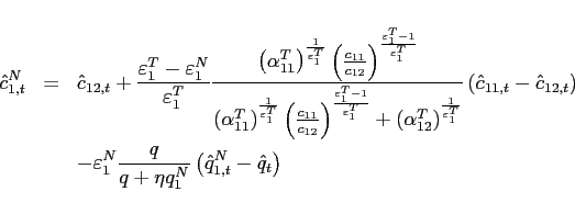
- for country 2:
is approximated by
![\begin{eqnarray*} c_{2,t}^{N}&=&c_{21,t}\frac{\alpha _{22}^{N}}{\alpha _{21}^{N}}\left[ \left( \alpha _{21}^{T}\right) ^{\frac{1}{\varepsilon_{2} ^{T}}}+\left( \alpha _{22}^{T}\right) ^{\frac{1}{\varepsilon_{2} ^{T}}}\left( \frac{c_{22,t}}{ c_{21,t}}\right) ^{\frac{\varepsilon_{2} ^{T}-1}{\varepsilon_{2} ^{T}}}\right] ^{ \frac{\varepsilon_{2} ^{T}-\varepsilon_{2} ^{N}}{\varepsilon_{2} ^{T}-1}}\left( \frac{ q_{2,t}^{N}}{\frac{1}{q_{t}}+\eta q_{2,t}^{N}}\right) ^{-\varepsilon_{2} ^{N}}\left( \frac{1}{\alpha _{21}^{T}}\right) ^{\frac{\varepsilon_{2} ^{N}}{ \varepsilon_{2} ^{T}}} \end{eqnarray*}](img128t.gif)
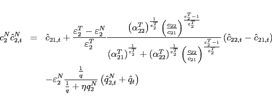
- for country 1:
- consumption optimal choice traded goods
- for country 1:
![\begin{eqnarray*} c_{12,t} &=& \frac{\alpha _{12}^{T}}{\alpha _{11}^{T}}\left( \frac{1+\eta q_{1,t}^{N}}{q_{t}+\eta q_{1,t}^{N}}\right) ^{\varepsilon_{1} ^{T}}c_{11,t} \ \hat{c}_{12,t} &=&\hat{c}_{11,t}+\left[ \frac{1}{1+\eta q_{1}^{N}}-\frac{ 1}{q+\eta q_{1}^{N}}\right] \varepsilon_{1} ^{T}\eta q_{1}^{N}\hat{q} _{1,t}^{N}-\frac{\varepsilon_{1} ^{T}}{q+\eta q_{1}^{N}}q\hat{q}_{t} \end{eqnarray*}](img131t.gif)
- for country 2:
![\begin{eqnarray*} c_{22,t}&=&\frac{\alpha _{22}^{T}}{\alpha _{21}^{T}}\left( \frac{\frac{1}{ q_{t}}+\eta q_{2,t}^{N}}{1+\eta q_{2,t}^{N}}\right) ^{\varepsilon_{2} ^{T}}c_{21,t} \ \hat{c}_{22,t}&=&\hat{c}_{21,t}+\left[ \frac{1}{\frac{1}{q}+\eta q_{2}^{N}} -\frac{1}{1+\eta q_{2}^{N}}\right] \varepsilon_{2} ^{T}\eta q_{2}^{N}\hat{q} _{2,t}^{N}-\frac{\varepsilon_{2} ^{T}}{\frac{1}{q}+\eta q_{2}^{N}}\frac{1}{q} \hat{q}_{t} \end{eqnarray*}](img133t.gif)
- for country 1:
- definition

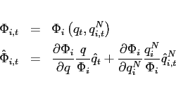
- for country 1:
![\begin{eqnarray*} \frac{\partial \Phi _{1}}{\partial q}\frac{q}{\Phi _{1}}=-\frac{\frac{c_{12} }{c_{1}^{N}}q}{\left[ \left( 1+\eta q_{1}^{N}\right) \frac{c_{11}}{c_{12}} +\left( q+\eta q_{1}^{N}\right) \right] \frac{c_{12}}{c_{1}^{N}}+q_{1}^{N}} \mbox{ and } \frac{\partial \Phi _{1}}{\partial q_{1}^{N}}\frac{q_{1}^{N}}{\Phi _{1}}= \frac{\partial \Phi _{1}}{\partial q}\frac{q}{\Phi _{1}}\frac{y_{1}^{N}q_{1}^{N}}{c_{12} q} \end{eqnarray*}](img137t.gif)
- for country 2:
![\begin{eqnarray*} \frac{\partial \Phi _{2}}{\partial q}\frac{q}{\Phi _{2}}=\frac{\frac{c_{21}}{ c_{2}^{N}}\frac{1}{q}}{\left[ \left( \frac{1}{q}+\eta q_{2}^{N}\right) \frac{ c_{21}}{c_{22}}+\left( 1+\eta q_{2}^{N}\right) \right] \frac{c_{22}}{ c_{2}^{N}}+q_{2}^{N}} \mbox{ and } \frac{\partial \Phi _{2}}{\partial q_{2}^{N}}\frac{q_{2}^{N}}{\Phi _{2}}=- \frac{y_{2}^{N}q_{2}^{N}}{c_{21}\frac{1}{q}}\frac{\partial \Phi _{2}}{\partial q}\frac{q}{\Phi _{2}} \end{eqnarray*}](img139t.gif)
- for country 1:
- definition

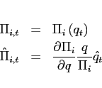
- for country 1:

- for country 2:

- for country 1:
- real exchange rate
is approximated by


- Cobb-Douglas production function with traded goods for country
 :
is approximated by
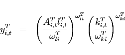

- optimal labor input choices traded goods for country
 :
is approximated by

- optimal capital input choices traded goods for country
 :
is approximated by

- Cobb-Douglas production function with non-traded goods for
country
 :
is approximated by
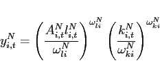

- optimal labor input choices non-traded goods for country
 :
is approximated by
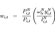

- optimal capital input choices non-traded goods for country
 :
is approximated by
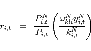

- labor market clearing for country
 :
is approximated by

- capital market clearing for country
 :
is approximated by

- goods market clearing non-traded goods for country
 :
is approximated by

- goods market clearing for good 2:
is approximated by


These equations can be rewritten in terms of the three state
variables
![]() ,
, ![]() ,
and
,
and ![]() .
.
C Appendix: Overlapping Generations Model
This appendix merges the framework with overlapping generations of infinitely lived households by Weil (1989) and Ghironi (2006) with the model presented in the main text. Absent Ricardian equivalence, the steady state level of the net foreign asset position can be shown to be unique. Furthermore, the local dynamics of the net foreign asset position are stationary.
C.1 The Model
Each household consumes, supplies labor, and holds financial
assets. Households are born on different dates owning no assets,
but they own the present discounted value of their labor income.
The number of households in country ![]()
![]() grows over time at the exogenous rate
grows over time at the exogenous rate ![]() , i.e.,
, i.e.,
![]() . The
utility function of each household is assumed to be of the
Cobb-Douglas type. Capital is no longer accumulated by households
directly, but through capital producers. Households can purchase
shares in these and all other firms that produce in their country
of residence. To allow the intertemporal elasticity of substitution
. The
utility function of each household is assumed to be of the
Cobb-Douglas type. Capital is no longer accumulated by households
directly, but through capital producers. Households can purchase
shares in these and all other firms that produce in their country
of residence. To allow the intertemporal elasticity of substitution ![]() to differ from 1 as in Ghironi (2006), aggregation requires perfect
foresight.
to differ from 1 as in Ghironi (2006), aggregation requires perfect
foresight.
C.1.1 Individual Households
Consumers have identical preferences over the real consumption
index and leisure. At time ![]() , the
representative consumer in country
, the
representative consumer in country ![]() born in
period
born in
period
![]() maximizes
the intertemporal utility function:
maximizes
the intertemporal utility function:
|
(24) |
| (25) |
The final consumption of a representative household of country ![]() born in period
born in period ![]() at time
at time ![]() is denoted by
is denoted by ![]() .
The production of the final consumption good follows the same
process as outlined in the main text.
.
The production of the final consumption good follows the same
process as outlined in the main text. ![]() is
the labor supply of such a household. The bond holdings are denoted
by
is
the labor supply of such a household. The bond holdings are denoted
by ![]() .
.
![]() are the household's holdings
of the domestic stock, that sells at the price
are the household's holdings
of the domestic stock, that sells at the price
![]() and pays the dividend
and pays the dividend
![]() . The supply of the stock is
normalized to 1.
. The supply of the stock is
normalized to 1.
Household choices for consumption, leisure, and asset holdings must satisfy the following first order conditions:
 |
(26) |
 |
(27) |
 |
(28) |
where the return of the stock is given by
 .
.
C.1.2 Firms
While I assume that the production structure of the economy is unchanged relative to the main text, capital is held by capital producers. These firms buy the investment good, augment the existing capital stock, and rent out capital to the producers of traded and non-traded goods. They also pay a dividend to the stockholders. The optimization problem of the capital producers is given by:
|
(29) |
![]() is the pricing kernel used
by the capital producers to discount future profits. The capital
used in time
is the pricing kernel used
by the capital producers to discount future profits. The capital
used in time ![]() production,
production, ![]() , and
investment,
, and
investment, ![]() , are expressed as per capita
averages. The average per capital dividend payment is denoted by
, are expressed as per capita
averages. The average per capital dividend payment is denoted by
![]() and satisfies
and satisfies
![]() . The
optimality condition for the capital producer is therefore given
by:
. The
optimality condition for the capital producer is therefore given
by:
![$\displaystyle \frac{Q_{i,t_{0}\vert t+1}}{Q_{i,t_{0}\vert t}}\frac{P_{i,t+1}^{c}}{ P_{i,t}^{c}}\frac{\Phi _{i,t+1}}{\Phi _{i,t}}\frac{\Pi _{i,t}}{\Pi _{i,t+1}^{I}}\left[ \Pi _{i,t+1}r_{i,t+1}+\left( 1-\delta \right) \right]=1.$](img216t.gif) |
(30) |
C.1.3 Aggregation
If the population at time ![]() is
is ![]() , aggregate per capita consumption in country
, aggregate per capita consumption in country ![]() satisfies
satisfies
![\begin{equation*} c_{i,t}=\frac{1}{\left( 1+n_{i}\right) ^{t}}\left[ \begin{array}{c} \frac{n_{i}}{\left( 1+n_{i}\right) ^{t+1}}c_{i,t}^{-t}+...+\frac{n_{i}}{\left( 1+n_{i}\right) ^{2}}c_{i,t}^{-1}+\frac{n_{i}}{1+n_{i}}c_{i,t}^{0} \ +nc_{i,t}^{1}+n_{i}\left( 1+n_{i}\right) c_{i,t}^{2}+...+n_{i}\left( 1+n_{i}\right) ^{t-1}c_{i,t}^{t} \end{array}\right]. \end{equation*}](img220t.gif)
Aggregate per capita labor supply equations are obtained by aggregating labor-leisure tradeoff equations across generations and dividing by the total population at each point in time. The aggregate per capita labor-leisure tradeoff satisfies
 |
(31) |
From (27) and (31) the price of the bond can be shown to satisfy
 |
(32) |
under perfect foresight.
To obtain the aggregate per capita budget constraint, note that the stock is in fixed supply. Thus,
 |
(33) |
Remains to determine the consumption of the newly born
generation in period ![]() . Defining total asset
holdings of generation
. Defining total asset
holdings of generation ![]() in period
in period ![]() by
by
 |
(34) |
the budget constraint of a generation ![]() household is
written as
household is
written as
 |
(35) |
Iterating forward on equation (35) and invoking the appropriate transversality condition, the budget constraint can be shown to satisfy
 |
(36) |
with
 |
(37) |
 |
(38) |
using the fact that
 |
|
| (39) |
As newly born agents do not hold financial assets, their consumption is given by
 |
(46) |
Note, in general the consumption of newly born households differs from the aggregate per capita consumption. Hence, the steady states of the model with overlapping generations differ from those obtained in the representative agents model.
D Appendix: Nominal and Real Rigidities
This appendix lays out the model with nominal and real rigidities. Following the influential work of Christiano, Eichenbaum, and Evans (1999) and Smets and Wouters (2003), the model features sticky wages and prices, consumption habits, and investment adjustment costs. Wage and price contracts are modeled as in Calvo (1983) and Yun (1996). Unless noted otherwise, the modeling features introduced in the main text remain unchanged. As in the main text, variables are expressed in per capita terms.
D.1 Additional Modeling Features
Wages A continuum of monopolistically competitive
households (indexed on the unit interval) supplies differentiated
labor services to the intermediate goods-producing sector. A
representative labor aggregator combines the households' labor
hours in the same proportions as firms would choose. This labor
index ![]() has the Dixit-Stiglitz form:
has the Dixit-Stiglitz form:
![\begin{displaymath} l_{t+j}=\left[ \int_{0}^{1}l_{t+j}\left( h\right) ^{\frac{1}{1+\theta^w _{i}}}dh \right] ^{1+\theta^w _{i}}, \end{displaymath}](img238t.gif) |
(41) |
where
![]() and
and ![]() is hours worked by a typical member of household
is hours worked by a typical member of household ![]() . The aggregator minimizes the cost of
producing a given amount of the aggregate labor index, taking each
household's wage rate
. The aggregator minimizes the cost of
producing a given amount of the aggregate labor index, taking each
household's wage rate
![]() as given. One unit of
the labor index sells at the unit cost
as given. One unit of
the labor index sells at the unit cost ![]() :
:
![\begin{displaymath} W_{t+j}=\left[ \int_{0}^{1}W_{t+j}{}\left( h\right) ^{\frac{-1}{\theta^w _{i}}}dh \right] ^{-\theta^w _{i}}. \end{displaymath}](img244t.gif) |
(42) |
![]() is referred to as the aggregate wage
index. The aggregator's demand for the labor services of household
is referred to as the aggregate wage
index. The aggregator's demand for the labor services of household ![]() satisfies:
satisfies:
![\begin{displaymath} l_{i,t+j}\left( h\right) =\left[ \frac{W_{i,t+j}\left( h\right) }{W_{i,t+j}}\right] ^{-\frac{1+\theta^w _{i}}{\theta^w _{i}}}l_{i,t+j}. \end{displaymath}](img247t.gif) |
(43) |
The utility functional of a typical member of household h is:
|
(44) |
where the discount factor ![]() satisfies
satisfies
![]() As in
Smets and Wouters (2003), I allow for the possibility of external
habits. At date
As in
Smets and Wouters (2003), I allow for the possibility of external
habits. At date ![]() , a member of household
, a member of household ![]() cares about consumption relative to lagged
per capita consumption
cares about consumption relative to lagged
per capita consumption ![]() .
. ![]() is a preference shock that follows an AR(1)
process. Furthermore, the period utility function depends on labor
is a preference shock that follows an AR(1)
process. Furthermore, the period utility function depends on labor
![]() and the
end-of-period real money balances,
and the
end-of-period real money balances,
![]() . The budget
constraint of a member of household h is given by:
. The budget
constraint of a member of household h is given by:
|
(45) |
The left hand side of the budget constraint summarizes the expenditures for consumption, investment (plus investment adjustment costs), expenditure and income from domestically-issued and traded bonds, government bonds, and the internationally-traded bond (plus portfolio cost). The right hand side provides information about the agent's labor and capital income, profits, and transfers.
Household wages are determined by Calvo-style staggered
contracts subject to static wage indexation. In particular, with
probability
![]() , each household is allowed to
reoptimize its wage contract. If a household is not allowed to
reoptimize its wage rate, it sets its wage according to
, each household is allowed to
reoptimize its wage contract. If a household is not allowed to
reoptimize its wage rate, it sets its wage according to
![]() with
with
![]() .
.
![]() is the actual wage inflation
rate and
is the actual wage inflation
rate and ![]() is the steady state inflation rate.
is the steady state inflation rate. ![]() is referred to as the wage
indexation parameter. A household who is resetting its wage in
period
is referred to as the wage
indexation parameter. A household who is resetting its wage in
period ![]() chooses
chooses ![]() such
that:
such
that:
![\begin{eqnarray*} 0 &=&-\mathbb{E}_{t}\sum_{j=0}^{\infty }\left( \beta _{i}\xi _{i}^{w}\right) ^{j}\left[ \chi _{0i}(l_{i,t+j}\left( h\right) )^{-\chi_{i} } \left( -\frac{1+\theta^w _{i}}{ \theta^w _{i}}\right) \left[ \frac{V_{i,t,j}^{W}W^*_{i,t}\left( h\right) }{ W_{i,t+j}}\right] ^{-\frac{1+\theta^w _{i}}{\theta^w _{i}}}\frac{l_{i,t+j}}{ W^*_{i,t}\left( h\right) }\right] \ &&+\mathbb{E}_{t}\sum_{j=0}^{\infty }\left( \beta _{i}\xi _{i}^{w}\right) ^{j}\left[\left( 1-\tau _{i}^{w}\right) \lambda _{i,t+j}\left( h\right) V_{i,t,j}^{W}W^*_{i,t}\left( h\right) \left( -\frac{1+\theta^w _{i}}{ \theta^w _{i}}\right) \left[ \frac{V_{i,t,j}^{W}W^*_{i,t}\left( h\right) }{ W_{i,t+j}}\right] ^{-\frac{1+\theta^w _{i}}{\theta^w _{i}}}\frac{l_{i,t+j}}{ W^*_{i,t}\left( h\right) }\right] \ &&+\mathbb{E}_{t}\sum_{j=0}^{\infty }\left( \beta _{i}\xi _{i}^{w}\right) ^{j}\lambda _{i,t+j}\left( h\right) \left( 1-\tau _{i}^{w}\right) V_{i,t,j}^{W}l_{i,t+j}\left( h\right), \end{eqnarray*}](img272t.gif)
where
![]() and
and
![]() for
for ![]() . Since households have access to
complete insurance markets domestically, the marginal utility of
wealth
. Since households have access to
complete insurance markets domestically, the marginal utility of
wealth
![]() is constant
across households. Thus, I drop the dependence of this variable on
h. Furthermore, the assumption of complete markets implies that all
households that reoptimize in period
is constant
across households. Thus, I drop the dependence of this variable on
h. Furthermore, the assumption of complete markets implies that all
households that reoptimize in period ![]() choose the
same wage rate
choose the
same wage rate
![]() Hence:
Hence:
|
(46) |
The real wage expressed in terms of country i's traded good evolves according to
 ![$\displaystyle \left[ \left( 1-\xi _{i}^{w}\right) \left( \frac{ W^*_{i,t+j} }{P_{ii,t+j}}\right) ^{\frac{-1}{\theta^w _{i}}}+\xi _{i}^{w}\left( \frac{\bar{\omega} _{i,t+j-1}}{\pi _{ii,t+j}}\frac{W_{i,t+j-1}}{P_{ii,t+j-1} }\right) ^{\frac{-1}{\theta^w _{i}}}\right] ^{-\theta^w _{i}}$](img294t.gif) |
(47) |
with
![]() .
.
Prices Both for traded and non-traded goods, there is a
continuum of differentiated intermediate goods in country ![]() indexed by
indexed by
![]() , each produced by a single
monopolistically competitive firm. Deviating from the main text, I
assume that individual varieties are traded internationally rather
than the final aggregate. Goods with index
, each produced by a single
monopolistically competitive firm. Deviating from the main text, I
assume that individual varieties are traded internationally rather
than the final aggregate. Goods with index
![]() are traded.
Consumption and investment varieties are interchangeable. The use
of the index h in the description of prices is unrelated to its use
in the description of wages.
are traded.
Consumption and investment varieties are interchangeable. The use
of the index h in the description of prices is unrelated to its use
in the description of wages.
Let
![]() be the overall
quantity produced by firm
be the overall
quantity produced by firm ![]() of the traded goods
producers using a
of the traded goods
producers using a ![]() technology. Firms operate
in perfectly competitive factor markets for aggregate capital and
the labor aggregate and thus operate with the same capital to labor
ratio. Denoting individual labor and capital demands by
technology. Firms operate
in perfectly competitive factor markets for aggregate capital and
the labor aggregate and thus operate with the same capital to labor
ratio. Denoting individual labor and capital demands by
![]() and
and
![]() , respectively,
and aggregate labor and capital demand by
, respectively,
and aggregate labor and capital demand by
![]() and
and
![]() , I
define aggregate output as:
, I
define aggregate output as:
![\begin{eqnarray*} &&y_{i,t+j}^{T} =\int_{0}^{1}y_{i,t+j}^{T}\left( h\right) dh=\left[ \left( \omega _{li}^{T}\right) ^{1-\kappa ^{T}}\left( \frac{\omega _{ki}^{T}}{ \omega _{li}^{T}}\right) ^{\kappa ^{T}}\left( \frac{w_{i,t+j}}{ A_{i,t+j}^{T}r_{i,t+j}}\right) ^{\frac{\kappa ^{T}}{\kappa ^{T}-1}}+\left( \omega _{ki}^{T}\right) ^{1-\kappa ^{T}}\right] ^{\frac{1}{\kappa ^{T}} }k_{i,t+j}^{T} \ &&\mbox{if }\kappa_{i} ^{T}<1\mbox{, and} \notag \ &&y_{i,t+j}^{T} =\int_{0}^{1}y_{i,t+j}^{T}\left( h\right) dh=\frac{1}{ 1-\omega _{li}^{T}}\left( A_{i,t+j}^{T}\frac{r_{i,t+j}}{w_{i,t+j}}\right) ^{\omega _{li}^{T}}k_{i,t+j}^{T}\ &&\mbox{if }\kappa_{i} ^{T}=0. \notag \end{eqnarray*}](img306t.gif)
Home and foreign prices of the intermediate goods are determined
by Calvo-style staggered contracts. Each period, a firm of country
1's traded goods sector faces a constant probability
![]() of being able to reoptimize
its price at home and
of being able to reoptimize
its price at home and
![]() probability of being able to
reoptimize its price abroad. These probabilities are assumed to be
independent across firms, time, and countries. For country 2 the
respective probabilities are
probability of being able to
reoptimize its price abroad. These probabilities are assumed to be
independent across firms, time, and countries. For country 2 the
respective probabilities are
![]() and
and
![]() . Similar to the behavior of
wages, firms that are not allowed to reoptimize their price in the
current period, adjust their price by a geometric average of the
actual inflation rate of the previous period (with weight
. Similar to the behavior of
wages, firms that are not allowed to reoptimize their price in the
current period, adjust their price by a geometric average of the
actual inflation rate of the previous period (with weight
![]() ,
, ![]() and
and ![]() ) and the steady state inflation rate
) and the steady state inflation rate ![]() (with weight
(with weight
![]() ,
, ![]() and
and ![]() ). I denote this average by
). I denote this average by
 .
.
I define the following aggregates of consumer and investment demand for the varieties produced in country 1:
![\begin{eqnarray*} c_{11,t+j} &=&\left[ \int_{0}^{1}c_{11,t+j}\left( h\right) ^{\frac{1}{1+\theta _{1}^{pT}}}dh\right] ^{1+\theta _{1}^{pT}} \mbox{ and } c_{21,t+j} =\bar{h}_{1}^{-\theta _{1}^{pT}}\left[ \int_{0}^{\bar{h} _{1}}c_{21,t+j}\left( h\right) ^{\frac{1}{1+\theta _{1}^{pT}}}dh\right] ^{1+\theta _{1}^{pT}}, \ x_{11,t+j} &=&\left[ \int_{0}^{1}x_{11,t+j}\left( h\right) ^{\frac{1}{1+\theta _{1}^{pT}}}dh\right] ^{1+\theta _{1}^{pT}} \mbox{ and } x_{21,t+j} = \bar{h}_{1}^{-\theta _{1}^{pT}}\left[ \int_{0}^{\bar{h} _{1}}x_{21,t+j}\left( h\right) ^{\frac{1}{1+\theta _{1}^{pT}}}dh\right] ^{1+\theta _{1}^{pT}}, \end{eqnarray*}](img319t.gif)
and the associated demand equations:
![\begin{eqnarray*} c_{11,t+j}\left( h\right) =\left[ \frac{P_{11,t+j}(h)}{P_{11,t+j}}\right] ^{\frac{-\left( 1+\theta _{1}^{pT}\right) }{\theta _{1}^{pT}}}c_{11,t+j} \mbox{ and } c_{21,t+j}\left( h\right) =\frac{1}{\bar{h}_{1}}\left( \frac{P_{21,t+j}(h)}{P_{21,t+j}}\right) ^{-\frac{1+\theta _{1}^{pT}}{\theta _{1}^{pT}}}c_{21,t+j}, \ x_{11,t+j}\left( h\right) =\left[ \frac{P_{11,t+j}(h)}{P_{11,t+j}}\right] ^{\frac{-\left( 1+\theta _{1}^{pT}\right) }{\theta _{1}^{pT}}}x_{11,t+j} \mbox{ and } x_{21,t+j}\left( h\right) =\frac{1}{\bar{h}_{1}}\left( \frac{P_{21,t+j}(h)}{P_{21,t+j}}\right) ^{-\frac{1+\theta _{1}^{pT}}{\theta _{1}^{pT}}}x_{21,t+j}. \end{eqnarray*}](img320t.gif)
The aggregator
![$P_{11,t+j} =\left[ \int_{0}^{1}\left[ P_{11,t+j}(h)\right] ^{-\frac{1}{\theta_{1}^{pT}}}dh\right] ^{-\theta _{1}^{pT}} $](img321t.gif) for domestically produced varieties implies:
for domestically produced varieties implies:
![\begin{eqnarray*} 1 &=&\left( 1-\xi _{11}^{pT}\right) \left[ \frac{P_{11,t+j}^{\ast }}{P_{11,t+j}} \right] ^{-\frac{1}{\theta _{1}^{pT}}}+\xi _{11}^{pT}\left[ \frac{\bar{\pi} _{11,t+j-1}}{\pi _{11,t+j}}\right] ^{- \frac{1}{\theta _{1}^{pT}}}, \end{eqnarray*}](img322t.gif)
where
![]() is the price set by those
firms that reoptimize in period
is the price set by those
firms that reoptimize in period ![]() and
and
![]() . Reoptimizing
firms choose to set the same price since marginal costs are
identical across firms.
. Reoptimizing
firms choose to set the same price since marginal costs are
identical across firms.
With respect to the export price index, ![]() denotes the price index in the currency of country 2 (local
currency) and
denotes the price index in the currency of country 2 (local
currency) and
![]() denotes the price index in
the currency of country 1 (exporter currency):
denotes the price index in
the currency of country 1 (exporter currency):
![\begin{eqnarray*} P_{21,t+j} &=&\left[ \frac{1}{\bar{h}_{1}}\int_{0}^{\bar{h}_{1}}\left( P_{21,t+j}(h)\right) ^{-\frac{1}{\theta _{1}^{pT}}}dh\right] ^{-\theta _{1}^{pT}}, \ 1 &=&\left[ \left( 1-\xi _{21}^{pT}\right) \left[ \frac{P_{21,t+j}^{\ast }}{ P_{21,t+j}}\right] ^{-\frac{1}{\theta _{1}^{pT}}}+\xi _{21}^{pT}\left( \frac{ \bar{\pi} _{21,t+j-1}}{\pi _{21,t+j}}\right) ^{-\frac{1}{\theta _{1}^{pT}}}\right] ^{-\theta _{1}^{pT}}, \ \tilde{P}_{21,t+j} &=&\left[ \frac{1}{\bar{h}_{1}}\int_{0}^{\bar{h}_{1}}\left( \tilde{P}_{21,t+j}(h)\right) ^{-\frac{1}{\theta _{1}^{pT}}}dh\right] ^{-\theta _{1}^{pT}}, \ 1 &=&\left[ \left( 1-\xi _{21}^{pT}\right) \left[ \frac{\tilde{P} _{21,t+j}^{\ast }}{\tilde{P}_{21,t+j}}\right] ^{-\frac{1}{\theta _{1}^{pT}}}+\xi _{21}^{pT}\left( \frac{\bar{\tilde{\pi}}_{21,t+j-1} }{\tilde{\pi}_{21,t+j}}\right) ^{-\frac{1}{\theta _{1}^{pT}}} \right] ^{-\theta _{1}^{pT}}, \end{eqnarray*}](img328t.gif)
where
![]() and
and
 . In addition, I define the price dispersion functions:
![\begin{eqnarray*} \Delta _{11,t+j} &=&\int_{0}^{1}\left[ \frac{P_{11,t+j}(h)}{P_{11,t+j}}\right] ^{ \frac{-\left( 1+\theta _{1}^{pT}\right) }{\theta _{1}^{pT}}}dh, \ \Delta _{11,t+j} &=&\left( 1-\xi _{11}^{pT}\right) \left[ \frac{P_{11,t+j}^{\ast }}{P_{11,t+j}}\right] ^{\frac{-\left( 1+\theta _{1}^{pT}\right) }{\theta _{1}^{pT}}}+\xi _{11}^{pT}\left[ \frac{\bar{\pi} _{11,t+j-1}} {\pi _{11,t+j}}\right] ^{\frac{-\left( 1+\theta _{1}^{pT}\right) }{\theta _{1}^{pT}}}\Delta _{11,t+j-1}, \ \Delta _{21,t+j} &=&\frac{1}{\bar{h}_{1}}\int_{0}^{\bar{h}_{1}}\left( \frac{ P_{21,t+j}(h)}{P_{21,t+j}}\right) ^{-\frac{1+\theta _{1}^{pT}}{\theta _{1}^{pT}}}dh,\ \Delta _{21,t+j} &=&\left( 1-\xi _{21}^{pT}\right) \left[ \frac{P_{21,t+j}^{\ast }}{P_{21,t+j}}\right] ^{-\frac{1+\theta _{1}^{pT}}{\theta _{1}^{pT}}}+\xi _{21}^{pT}\left[ \frac{\bar{\pi} _{21,t+j-1}}{\pi _{21,t+j}}\right] ^{-\frac{1+\theta _{1}^{pT}}{\theta _{1}^{pT}}}\Delta _{21,t+j-1}, \end{eqnarray*}](img331t.gif)
and equivalently for
![]() . As the market
clearing condition for each variety
. As the market
clearing condition for each variety ![]() satisfies:
satisfies:
![\begin{eqnarray*} y_{1,t+j}^{T}\left( h\right) &=&\left[ c_{11,t+j}\left( h\right) +x_{11,t+j}\left( h\right) \right] +\left[ c_{21,t+j}\left( h\right) +x_{21,t+j}\left( h\right) \right] \upsilon_2, \ \end{eqnarray*}](img334t.gif)
in the aggregate one obtains under the assumption of local currency pricing:
![\begin{eqnarray*} y_{1,t+j}^{T} &=&\left( \int_{0}^{1}\left[ \frac{P_{11,t+j}(h)}{P_{11,t+j}}\right] ^{\frac{ -\left( 1+\theta _{1}^{pT}\right) }{\theta _{1}^{pT}}}dh\right) \left[ c_{11,t+j}+x_{11,t+j}\right] \ && +\left( \frac{1}{\bar{h}_{1}}\int_{0}^{\bar{h} _{1}}\left( \frac{P_{21,t+j}(h)}{P_{21,t+j}}\right) ^{-\frac{1+\theta _{1}^{pT}}{ \theta _{1}^{pT}}} dh \right) \left[ c_{21,t+j}+x_{21,t+j}\right] \ &=&\Delta _{11,t+j}\left[ c_{11,t+j}+x_{11,t+j}\right] +\Delta _{21,t+j}\left[ c_{21,t+j}+x_{21,t+j}\right]. \end{eqnarray*}](img335t.gif)
The parameter ![]() adjusts for the differences in
country size.
adjusts for the differences in
country size.
As before the consumption of traded goods requires distribution services in the form of the non-traded goods. Market clearing for the non-traded good is derived from:

where
![\begin{eqnarray*} \Delta _{i,t}^{N} &=&\int \left[ \frac{P_{i,t}(h)}{P_{i,t}}\right] ^{\frac{ -\left( 1+\theta _{n}^{pN}\right) }{\theta _{n}^{pN}}}dh \end{eqnarray*}](img338t.gif)
which follows a similar law of motion as the dispersion measure of traded goods prices.
Remains to define the optimization problem of firms. A traded goods
producer firm located in country 1 that sells
domestically chooses its price ![]() to
maximize:
to
maximize:
![\begin{displaymath} E_{t}\sum_{j=0}^{\infty }\xi _{11}^{pT}\psi _{1,t,t+j}\left[ V_{11,t,j}^{pT}\left( 1+\tau _{11}\right) P_{11,t}\left( h\right) y_{11,t+j}^{T}\left( h\right) -MC_{1,t+j}y^T_{11,t+j}\left( h\right) \right], \end{displaymath}](img341t.gif) |
(48) |
where
| (49) | |
| (50) | |
![$\displaystyle \left[ \frac{V_{11,t,j}^{pT}P_{11,t}(h)}{ P_{11,t+j}}\right] ^{\frac{-\left( 1+\theta _{1}^{pT}\right) }{\theta _{1}^{pT}}}y^T_{11,t+j}.$](img350t.gif) |
(51) |
![]() is a price subsidy.
is a price subsidy.
![]() is the stochastic discount
factor that relates to the marginal utility of wealth as defined
below. Using
is the stochastic discount
factor that relates to the marginal utility of wealth as defined
below. Using
 , the first order condition implies:
![\begin{displaymath} E_{t}\sum_{j=0}^{\infty }\left( \xi _{11}^{pT}\right) ^{j}\psi _{1,t,t+j} \left[ V_{11,t,j}^{pT}\frac{1+\tau _{11}}{1+\theta _{1}^{pT}} P^{*}_{11,t}-MC_{1,t+j}\right] \frac{y^T_{11,t+j}\left( h\right)}{P^*_{11,t}} =0, \end{displaymath}](img354t.gif) |
(52) |
which can also be written as:
 |
(53) |
|
(54) |
|
(55) |
 |
(56) |
With respect to export pricing, I distinguish possibilities: producer currency pricing and local currency pricing. If country 1's exporters engage in producer currency pricing:
![\begin{displaymath} E_{t}\sum_{j=0}^{\infty }\xi _{21}^{pT}\psi _{1,t,t+j}\left[ \left( 1+\tau _{21}\right) \tilde{V}_{21,t,j}^{pT}\tilde{P}_{21,t}\left( h\right) -MC_{1,t+j} \right]y_{21,t+j}^{T}\left( h\right), \end{displaymath}](img372t.gif) |
(57) |
where
| (58) | |
| (59) | |
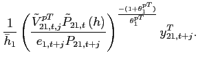 |
(60) |
Note, that I have defined
 and
and
 . Using
 , the first order condition implies:
![\begin{eqnarray*} &&E_{t}\sum_{j=0}^{\infty }\left( \xi _{21}^{pT}\right) ^{j}\psi _{1,t,t+j} \left[ \frac{1+\tau _{21}}{1+\theta _{1}^{pT}} \tilde{V} _{21,t,j}^{pT}\tilde{P}_{21,t}^* -MC_{1,t+j}\right] \frac{ y^T_{21,t+j}\left( h\right) }{\tilde{P}_{21,t}^{*} } =0, \end{eqnarray*}](img385t.gif)
or

Under local currency pricing, a firm maximizes:
![\begin{displaymath} E_{t}\sum_{j=0}^{\infty }\left( \xi _{21}^{pT}\right) ^{j}\psi _{1,t,t+j} \left[ \left( 1+\tau _{21}\right) V_{21,t,j}^{pT}P_{21,t}\left( h\right) e_{1,t+j} -MC_{1,t+j} \right]y_{21,t+j}\left( h\right), \end{displaymath}](img387t.gif) |
(61) |
where
| (62) | |
| (63) | |
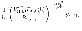 |
(64) |
Note, that I have used the definitions
![]() ,
,
 ,
,
![]() .
Using
.
Using
 , the first order condition implies:
![$\displaystyle E_{t}\sum_{j=0}^{\infty }\left( \xi _{21}^{pT}\right) ^{j}\psi _{1,t,t+j} \left[ \frac{1+\tau _{21}}{1+\theta _{1}^{pT}}V_{21,t,j}^{pT} P_{21,t}^{*}e_{1,t+j}-MC_{1,t+j}\right] \frac{y_{21,t+j}(h)}{P_{21,t}^{*}} =0,$](img401t.gif) |
(65) |
or
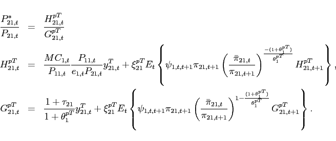
Similar expressions apply for country 2 and the non-traded goods sector.
D.2 Model Equations
D.2.1 Definitions
The following definitions are adopted.
- Real relative prices:
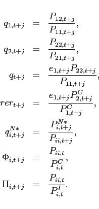
- Optimized relative prices:
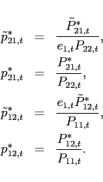
- Inflation terms:
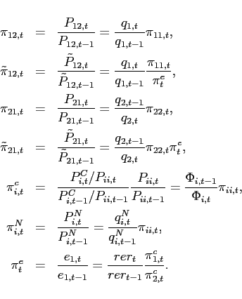
- Price updating:
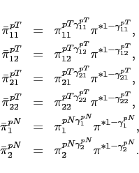
- Wages and wage inflation:
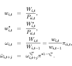
- Real marginal costs:
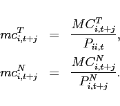
- Profits and assets:
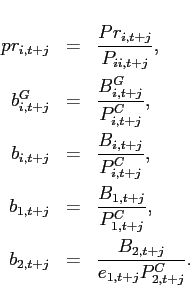
D.2.2 Model Equations
The following conditions need to be satisfied in the model with real and nominal rigidities.
- Labor choice:
![\begin{eqnarray*} \frac{H^{W}_{i,t}}{G^{W}_{i,t}} &=&\left( \frac{W^*_{i,t}}{P_{ii,t}}\right) ^{1-\frac{1+\theta^w _{i}}{\theta^w _{i}}\chi_{i} } \ H^{W}_{i,t} &=&\chi _{0i}\left( \left[ \frac{P_{ii,t}}{W_{i,t}}\right] ^{-\frac{1+\theta^w _{i}}{\theta^w _{i}}}l_{i,t}\right) ^{1-\chi_{i} }+\left( \beta _{i}\xi _{i}^{w}\right) ^{1}\mathbb{E}_{t}\left( \frac{\bar{\omega} _{i,t}}{ \pi _{ii,t+1}}\right) ^{-\frac{1+\theta^w _{i}}{\theta^w _{i}}\left( 1-\chi_{i} \right) }H^{W}_{i,t+1} \notag \ G^{W}_{i,t} &=&\frac{1-\tau _{i}^{w}}{1+\theta^w _{i}}\lambda _{i,t} P_{i,t}^{C}\Phi _{i,t} \left[ \frac{P_{ii,t}}{W_{i,t}}\right] ^{-\frac{ 1+\theta^w _{i}}{\theta^w _{i}}}l_{i,t} +\beta _{i}\xi _{i}^{w} \mathbb{E}_{t}\left( \frac{\bar{\omega} _{i,t}}{\pi _{ii,t+1}}\right) ^{\frac{-1}{ \theta^w _{i}}}G^{W}_{i,t+1} \notag \end{eqnarray*}](img411t.gif)
- Aggregate wage evolution
![\begin{eqnarray*} \frac{W_{i,t+j}}{P_{ii,t+j}} &=&\left[ \left( 1-\xi _{i}^{w}\right) \left( \frac{ W^*_{i,t+j} }{P_{ii,t+j}}\right) ^{\frac{-1}{\theta^w _{i}}}+\xi _{i}^{w}\left( \frac{\bar{\omega} _{i,t+j-1}}{\pi _{ii,t+j}}\frac{W_{i,t+j-1}}{P_{ii,t+j-1} }\right) ^{\frac{-1}{\theta^w _{i}}}\right] ^{-\theta^w _{i}} \end{eqnarray*}](img412t.gif)
- Marginal utility of consumption

- Investment choice

- Capital choice

Absent investment adjustment costs, i.e.,
 , it is
 and thus
- Capital accumulation

- Consumption budget constraint 1
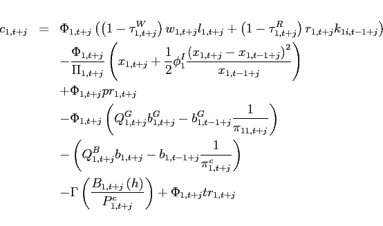
for country 2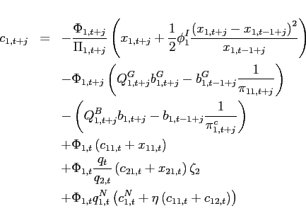
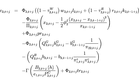
and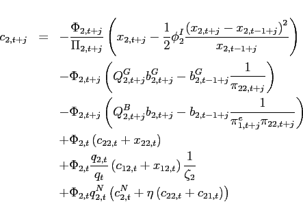

- Risk sharing condition: with adjustment costs

- Price of bond derived from country 1
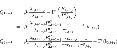
- Bond market clearing

- Investment aggregate: for country

![\begin{eqnarray*} x_{i,t+j}=\left[ \left( \alpha _{i1}^{I}\right) ^{\frac{1}{\varepsilon _{i}^{I}}}\left( x_{i1,t+j}\right) ^{\frac{\varepsilon _{i}^{I}-1}{ \varepsilon _{i}^{I}}}+\left( \alpha _{i2}^{I}\right) ^{\frac{1}{\varepsilon _{i}^{I}}}\left( x_{i2,t+j}\right) ^{\frac{\varepsilon _{i}^{I}-1}{ \varepsilon _{i}^{I}}}\right] ^{\frac{\varepsilon _{i}^{I}}{\varepsilon _{i}^{I}-1}} \end{eqnarray*}](img432t.gif)
- Investment optimal choices:
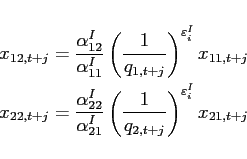
- Consumption aggregate over traded goods: for country

![\begin{eqnarray*} c_{i,t+j}^{T}=\left[ \left( \alpha _{i1}^{T}\right) ^{\frac{1}{\varepsilon _{i}^{T}}}\left( c_{i1,t+j}\right) ^{\frac{\varepsilon _{i}^{T}-1}{ \varepsilon _{i}^{T}}}+\left( \alpha _{i2}^{T}\right) ^{\frac{1}{\varepsilon _{i}^{T}}}\left( c_{i2,t+j}\right) ^{\frac{\varepsilon _{i}^{T}-1}{ \varepsilon _{i}^{T}}}\right] ^{\frac{\varepsilon _{i}^{T}}{\varepsilon _{i}^{T}-1}} \end{eqnarray*}](img435t.gif)
- Consumption aggregate over traded and non traded goods: for
country

![\begin{eqnarray*} c_{i,t+j}=\left[ \left( \alpha _{i1}^{N}\right) ^{\frac{1}{\varepsilon _{i}^{N}}}\left( c_{i,t+j}^{T}\right) ^{\frac{\varepsilon _{i}^{N}-1}{ \varepsilon _{i}^{N}}}+\left( \alpha _{i2}^{N}\right) ^{\frac{1}{\varepsilon _{i}^{N}}}\left( c_{i,t+j}^{N}\right) ^{\frac{\varepsilon _{i}^{N}-1}{ \varepsilon _{i}^{N}}}\right] ^{\frac{\varepsilon _{i}^{N}}{\varepsilon _{i}^{N}-1}} \end{eqnarray*}](img437t.gif)
- Consumption optimal choices non-traded goods: for country 1
and for country 2
![\begin{eqnarray*} c_{1,t+j}^{N}=c_{12,t+j}\frac{\alpha _{12}^{N}}{\alpha _{11}^{N}}\left[ \left( \alpha _{11}^{T}\right) ^{\frac{1}{\varepsilon _{i}^{T}}}\left( \frac{ c_{11,t+j}}{c_{12,t+j}}\right) ^{\frac{\varepsilon _{i}^{T}-1}{\varepsilon _{i}^{T}}}+\left( \alpha _{12}^{T}\right) ^{\frac{1}{\varepsilon _{i}^{T}}} \right] ^{\frac{\varepsilon _{i}^{T}-\varepsilon _{i}^{N}}{\varepsilon _{i}^{T}-1}}\left( \frac{q_{1,t+j}^{N}}{q_{1,t+j}+\eta q_{1,t+j}^{N}}\right) ^{-\varepsilon _{i}^{N}}\left( \frac{1}{\alpha _{12}^{T}}\right) ^{\frac{ \varepsilon _{i}^{N}}{\varepsilon _{i}^{T}}} \end{eqnarray*}](img439t.gif)
![\begin{eqnarray*} c_{2,t+j}^{N}=c_{21,t+j}\frac{\alpha _{22}^{N}}{\alpha _{21}^{N}}\left[ \left( \alpha _{21}^{T}\right) ^{\frac{1}{\varepsilon _{i}^{T}}}+\left( \alpha _{22}^{T}\right) ^{\frac{1}{\varepsilon _{i}^{T}}}\left( \frac{ c_{22,t+j}}{c_{21,t+j}}\right) ^{\frac{\varepsilon _{i}^{T}-1}{\varepsilon _{i}^{T}}}\right] ^{\frac{\varepsilon _{i}^{T}-\varepsilon _{i}^{N}}{ \varepsilon _{i}^{T}-1}}\left( \frac{q_{2,t+j}^{N}}{\frac{1}{q_{2,t+j}}+\eta q_{2,t+j}^{N}}\right) ^{-\varepsilon _{i}^{N}}\left( \frac{1}{\alpha _{21}^{T}}\right) ^{\frac{\varepsilon _{i}^{N}}{\varepsilon _{i}^{T}}} \end{eqnarray*}](img441t.gif)
- Consumption optimal choice traded goods: for country 1
for country 2
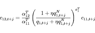
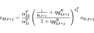
- Price definition
 : for country 1
for country 2
: for country 1
for country 2![\begin{eqnarray*} \Phi _{1,t+j}=\frac{\frac{c_{1,t+j}}{c_{1,t+j}^{N}}}{\left[ \left( 1+\eta q_{1,t+j}^{N}\right) \frac{c_{11,t+j}}{c_{12,t+j}}+\left( q_{1,t+j}+\eta q_{1,t+j}^{N}\right) \right] \frac{c_{12,t+j}}{c_{1,t+j}^{N}}+q_{1,t+j}^{N}} \end{eqnarray*}](img448t.gif)
![\begin{eqnarray*} \Phi _{2,t+j}=\frac{\frac{c_{2,t+j}}{c_{2,t+j}^{N}}}{\left[ \left( \frac{1}{ q_{2,t+j}}+\eta q_{2,t+j}^{N}\right) \frac{c_{21,t+j}}{c_{22,t+j}}+\left( 1+\eta q_{2,t+j}^{N}\right) \right] \frac{c_{22,t+j}}{c_{2,t+j}^{N}} +q_{2,t+j}^{N}} \end{eqnarray*}](img450t.gif)
- Price definition
 : for country 1
for country 2
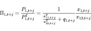
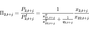
- Consumption real exchange rate
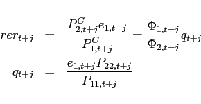
- Production traded goods: for country

![\begin{eqnarray*} y_{i,t+j}^{T} &=&\left[ \left( \omega _{li}^{T}\right) ^{1-\kappa _{i}^{T}}\left( A_{i,t+j}^{T}l_{i,t+j}^{T}\right) ^{\kappa _{i}^{T}}+\left( \omega _{ki}^{T}\right) ^{1-\kappa _{i}^{T}}\left( k_{i,t+j}^{T}\right) ^{\kappa _{i}^{T}}\right] ^{\frac{1}{\kappa _{i}^{T}}} \end{eqnarray*}](img458t.gif)
- Production non-traded goods: for country

![\begin{eqnarray*} y_{i,t+j}^{N} &=&\left[ \left( \omega _{li}^{N}\right) ^{1-\kappa _{i}^{N}}\left( A_{i,t+j}^{N}l_{i,t+j}^{N}\right) ^{\kappa _{i}^{N}}+\left( \omega _{ki}^{N}\right) ^{1-\kappa _{i}^{N}}\left( k_{i,t+j}^{N}\right) ^{\kappa _{i}^{N}}\right] ^{\frac{1}{\kappa _{i}^{N}}} \end{eqnarray*}](img460t.gif)
- Optimal labor input choices traded goods: for country


- Optimal capital input choices traded goods: for country

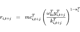
- Optimal labor input choices traded goods: for country


- Optimal capital input choices traded goods: for country

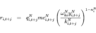
- Labor market clearing

- Capital market clearing

- Goods market clearing for good 1:
![\begin{eqnarray*} y_{1}^{T} &=&\Delta _{11,t}\left[ c_{11,t}+x_{11,t}\right] +\Delta _{21,t}\left[ c_{21,t}+x_{21,t}\right] \nu _{2} \end{eqnarray*}](img472t.gif)
- Evolution of dispersion index good 1: country 1
country 2 under producer currency pricing
 under local currency pricing

- Goods market clearing for good 2:
![\begin{eqnarray*} \nu _{2}y_{2}^{T}=\Delta _{12,t}\left[ c_{12,t}+x_{12,t}\right] +\Delta _{22,t}\left[ c_{22,t}+x_{22,t}\right] \nu _{2} \end{eqnarray*}](img480t.gif)
- Evolution of dispersion index good 2: country 2
country 1 under producer currency pricing
 under local currency pricing

- Goods market clearing non-traded goods: for country

![\begin{eqnarray*} y_{i,t+j}^{N} &=&\Delta _{i,t+j}^{N}\left[ c_{i,t+j}^{N}+\eta \left( c_{i1,t+j}+c_{i2,t+j}\right) \right] \end{eqnarray*}](img488t.gif)
- Evolution of dispersion index non-traded good
 :
:
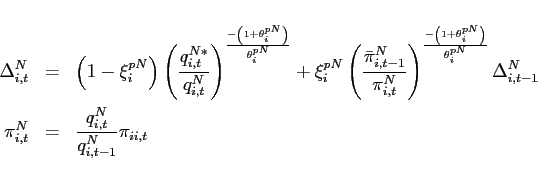
- Price indices good 1: country 1
for country 2: if producer currency pricing
 if local currency pricing

- Price indices good 2: country 2
for country 1: if producer currency pricing
 if local currency pricing

- Price index non-traded good

- Stochastic discount factors
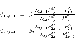
- Price for traded good country 1
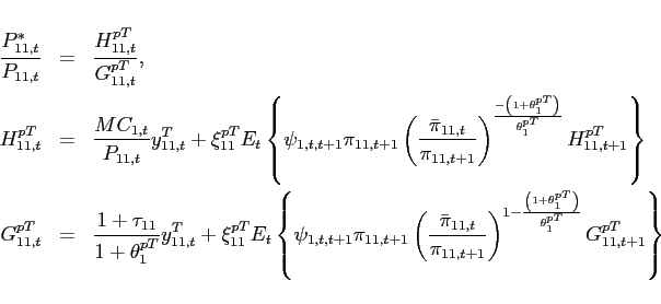
- Export price for traded good country 1:
producer currency pricing
local currency pricing
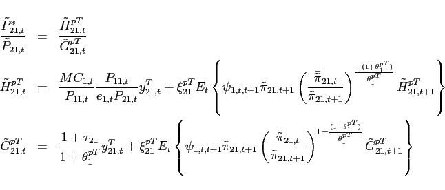
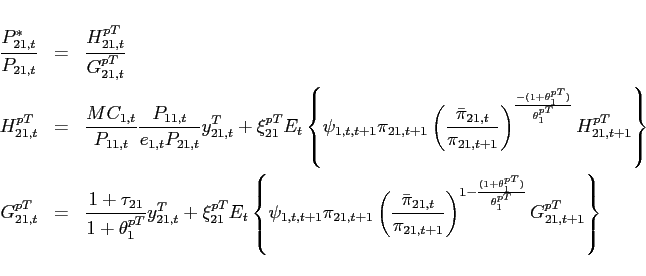
- Price for traded good country 2
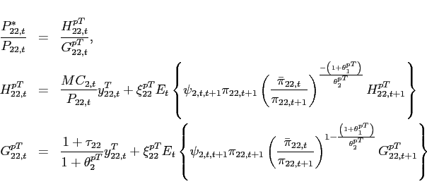
- Export price for traded good country 2:
producer currency pricing
local currency pricing
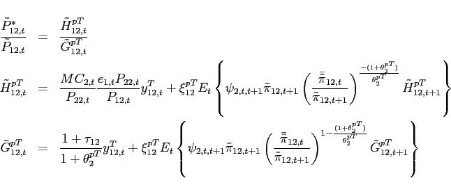
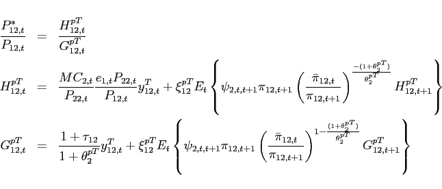
- Price for non-traded good country
 :
:
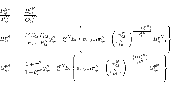
- Definition of real profits
 profits from
home activities
from exporting with producer currency pricing
profits from
home activities
from exporting with producer currency pricing![\begin{eqnarray*} Pr_{11,t} &=&\int_{0}^{1}\left( \left( 1+\tau _{11}\right) P_{11,t}\left( h\right) -MC_{1,t}\right) \left( c_{11,t}\left( h\right) +x_{11,t}\left( h\right) \right) dh \ pr_{11,t} &=&\left[ \left( 1+\tau _{11}\right) -mc_{1,t}\Delta _{11,t}^{T}\right] \left( c_{11,t}+x_{11,t}\right) \end{eqnarray*}](img518t.gif) with local currency pricing
with local currency pricing![\begin{eqnarray*} Pr_{21,t} &=&\int_{0}^{\bar{h}_{1}}\left( \left( 1+\tau _{21}\right) \tilde{P}_{21,t}\left( h\right) -MC_{1,t}\right) \left( c_{21,t}\left( h\right) +x_{21,t}\left( h\right) \right) \nu _{2}dh \ \frac{Pr_{21,t}}{P_{11,t}} &=&\left[ \left( 1+\tau _{21}\right) \frac{q_{t} }{q_{2,t}}-mc_{1,t}\Delta _{21,t}^{T}\right] \left( c_{21,t}+x_{21,t}\right) \nu _{2} \end{eqnarray*}](img519t.gif) and the non-traded goods
and the non-traded goods![\begin{eqnarray*} Pr_{21,t} &=&\int_{0}^{\bar{h}_{1}}\left( \left( 1+\tau _{21}\right) e_{1,t}P_{21,t}\left( h\right) -MC_{1,t}\right) \left( c_{21,t}\left( h\right) +x_{21,t}\left( h\right) \right) \nu _{2}dh \ \frac{Pr_{21,t}}{P_{11,t}} &=&\left[ \left( 1+\tau _{21}\right) \frac{q_{t} }{q_{2,t}}-mc_{1,t}\Delta _{21,t}^{T}\right] \left( c_{21,t}+x_{21,t}\right) \nu _{2} \end{eqnarray*}](img520t.gif) Consolidate household budget constraint
Consolidate household budget constraint![\begin{eqnarray*} \frac{Pr_{1,t}^{N}}{P_{11,t}}=q_{1,t}^{N}\left[ \left( 1+\tau _{1,t}^{N}\right) -mc_{1,t}^{N}\Delta _{1,t}^{N}\right] \left( c_{1,t}^{N}+\eta \left( c_{11,t}+c_{12,t}\right) \right) \end{eqnarray*}](img521t.gif)
![\begin{eqnarray*} &&\Phi _{1,t}\left( \left( 1-\tau _{1}^{W}\right) w_{1,t}l_{1,t}+\left( 1-\tau _{1}^{R}\right) r_{1,t}k_{1i,t-1}\right) +\Phi _{1,t}\left( pr_{1,t}+tr_{1,t}\right) \ &=&\Phi _{1,t}w_{1,t}l_{1,t}+\Phi _{1,t}r_{1,t}k_{1i,t-1} +\Phi _{1,t}\left[ 1-mc_{1,t}\Delta _{11,t}^{T}\right] \left( c_{11,t}+x_{11,t}\right) \ &&+\Phi _{1,t}\left[ \frac{q_{t}}{q_{2,t}}-mc_{1,t}\Delta _{21,t}^{T}\right] \left( c_{21,t}+x_{21,t}\right) \nu _{2} +\Phi _{1,t}q_{1,t}^{N}\left[ 1-mc_{1,t}^{N}\Delta _{1,t}^{N}\right] \left( c_{1,t}^{N}+\eta \left( c_{11,t}+c_{12,t}\right) \right) \ &=&+\Phi _{1,t}\left( c_{11,t}+x_{11,t}\right) +\Phi _{1,t}\frac{q_{t}}{q_{2,t}}\left( c_{21,t}+x_{21,t}\right) \nu _{2}\ &&+\Phi _{1,t}q_{1,t}^{N}\left( c_{1,t}^{N}+\eta \left( c_{11,t}+c_{12,t}\right) \right) \end{eqnarray*}](img522t.gif)
- Price of government debt

- Government budget constraint
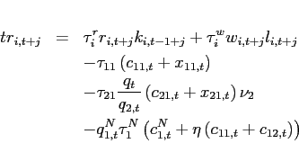
- Nominal interest rate

- Monetary policy
with the steady state inflation rate

 and the
steady state nominal interest rate
 .
.
References
Calvo, G. (1983). Staggered prices in a utility maximizing framework. Journal of Monetary Economics 12(3), 383�398.
Christiano, L. J., M. Eichenbaum, and C. L. Evans (1999). Monetary policy shocks: What have we learned and to what end?
Ghironi, F. (2006). Macroeconomic interdependence under incomplete markets. Journal of International Economics 70(2), 428�450.
Smets, F. and R. Wouters (2003). An estimated dynamic stochastic general equilibrium model of the euro area. Journal of the European Economic Association 1(5), 1123� 1175.
Weil, P. (1989). Overlapping families of infinitely-lived agents. Journal of Public Economics 38(2), 183�198.
Yun, T. (1996). Nominal price rigidity, money supply endogeneity and business cycles. Journal of Monetary Economics 37(2), 345�370.
Footnotes
1. If the discount factors were increasing in the level of consumption, ![]() would be negative and the dynamics around any deterministic steady state would be explosive. Return to text
would be negative and the dynamics around any deterministic steady state would be explosive. Return to text
This version is optimized for use by screen readers. Descriptions for all mathematical expressions are provided in LaTex format. A printable pdf version is available. Return to text

![$\displaystyle F_{i}^{T}\left( l_{i,t+j}^{T},k_{i,t+j}^{T}\right) =\left[ \left( \omega _{li}^{T}\right) ^{1-\kappa_{i} ^{T}}\left( A_{i,t+j}^{T}l_{i,t+j}^{T}\right) ^{\kappa_{i} ^{T}}+\left( \omega _{ki}^{T}\right) ^{1-\kappa_{i} ^{T}}\left( k_{i,t+j}^{T}\right) ^{\kappa_{i} ^{T}}\right] ^{\frac{1}{\kappa_{i} ^{T}}}$](img184.gif)

![$\displaystyle +\frac{\gamma}{\beta \Phi_1(q)} \left[1+\frac{1}{q} \right]\Delta b_{1,t}.$](img537.gif)


![$\displaystyle U_{t_{0}}^{v}=\sum_{t=t_{0}}^{\infty }\beta ^{t-t_{0}}\frac{\left[ \left( c_{i,t}^{v}\right) ^{\xi _{i}}\left( 1-l_{i,t}^{v}\right) ^{1-\xi _{i}}\right] ^{1-\sigma _{i}}-1}{1-\sigma _{i}}$](img563.gif)

![$\displaystyle +\frac{\gamma}{\beta \Phi_1(q)} \left[1+\frac{1}{q} \right]\Delta b_{1,t}.$](img49t.gif)


![$\displaystyle U_{t_{0}}^{v}=\sum_{t=t_{0}}^{\infty }\beta ^{t-t_{0}}\frac{\left[ \left( c_{i,t}^{v}\right) ^{\xi _{i}}\left( 1-l_{i,t}^{v}\right) ^{1-\xi _{i}}\right] ^{1-\sigma _{i}}-1}{1-\sigma _{i}}$](img190t.gif)


![$\displaystyle \mathbb{E}_{t}\sum_{j=0}^{\infty }\left( \beta _{i}\xi _{i}^{w}\right) ^{j}\chi _{0i}\left( \left[ V_{i,t,j}^{W}\frac{ P_{ii,t+j}}{W_{i,t+j}}\frac{P_{ii,t}}{P_{ii,t+j}}\right] ^{-\frac{1+\theta^w _{i}}{\theta^w _{i}}}l_{i,t+j}\right) ^{1-\chi_{i} } \notag$](img284t.gif)
![$\displaystyle \chi _{0i}\left( \left[ \frac{P_{ii,t}}{W_{i,t}}\right] ^{-\frac{1+\theta^w _{i}}{\theta^w _{i}}}l_{i,t}\right) ^{1-\chi_{i} }+\left( \beta _{i}\xi _{i}^{w}\right) ^{1}\mathbb{E}_{t}\left( \frac{\bar{\omega} _{i,t}}{ \pi _{ii,t+1}}\right) ^{-\frac{1+\theta^w _{i}}{\theta^w _{i}}\left( 1-\chi_{i} \right) }H^{W}_{i,t+1} \notag$](img286t.gif)
![$\displaystyle \mathbb{E}_{t}\sum_{j=0}^{\infty }\left( \beta _{i}\xi _{i}^{w}\right) ^{j}\frac{1-\tau _{i}^{w}}{1+\theta^w _{i}}\lambda _{i,t+j} P_{i,t+j}^{C}\Phi _{i,t+j}\left( \frac{P_{ii,t}}{ P_{ii,t+j}}V_{i,t,j}^{W}\right) \left[ V_{i,t,j}^{W}\frac{P_{ii,t+j}}{ W_{i,t+j}}\frac{P_{ii,t}}{P_{ii,t+j}}\right] ^{-\frac{1+\theta^w _{i}}{\theta^w _{i}}}l_{i,t+j} \notag$](img289t.gif)
![$\displaystyle \frac{1-\tau _{i}^{w}}{1+\theta^w _{i}}\lambda _{i,t} P_{i,t}^{C}\Phi _{i,t} \left[ \frac{P_{ii,t}}{W_{i,t}}\right] ^{-\frac{ 1+\theta^w _{i}}{\theta^w _{i}}}l_{i,t} +\beta _{i}\xi _{i}^{w} \mathbb{E}_{t}\left( \frac{\bar{\omega} _{i,t}}{\pi _{ii,t+1}}\right) ^{\frac{-1}{ \theta^w _{i}}}G^{W}_{i,t+1}. \notag$](img291t.gif)


