skip to main navigation skip to secondary navigation skip to content
Board of Governors of the Federal Reserve System
skip to content

FEDS Notes

Apr 2014

The FRB/US Model: A Tool for Macroeconomic Policy Analysis

Flint Brayton, Thomas Laubach, and David Reifschneider1 

Introduction
The FRB/US model of the U.S. economy is one of several that Federal Reserve Board staff consults for forecasting and the analysis of macroeconomic issues, including both monetary and fiscal policy. To improve public access to and understanding of the model, a new page has been introduced on the Federal Reserve Board's website from which interested users can download expanded FRB/US documentation; model equations, coefficients, and data; and sample simulation programs.2 

These simulation programs can be run by anyone with access to the EViews software package, a widely available commercial product. This note provides a brief summary of the main features of the model, illustrates some applications of the model using sample programs provided on the web page, and concludes with an overview of the contents of the web page. Because the model continues to undergo changes as both economic theory and empirical evidence evolve, any given model release reflects only the state of thinking at the time of the release.

The FRB/US Model: A Brief Overview
The FRB/US model is a large-scale model of the U.S. economy featuring optimizing behavior by households and firms as well as detailed descriptions of monetary policy and the fiscal sector. The model's large number of endogenous variables permits the study of the effects of a broad range of macroeconomic policies and exogenous shocks on real GDP and its major spending components; the unemployment rate and other key labor market indicators; several measures of inflation and relative prices; the main categories of national income; a detailed treatment of the government's account; and various interest rates, asset prices, and components of wealth. FRB/US has a neoclassical core that combines a production function with endogenous and exogenous supplies of production factors and key aspects of household preferences such as impatience. To account for cyclical fluctuations, the model features rigidities that apply to many decisions made by households and firms; these rigidities enable the model to generate gradual responses of macroeconomic variables to a wide range of exogenous shocks that are consistent with the economic data.3 

Although a detailed description of the model's equations is beyond the scope of this note, a number of resources are available on the new web page. Here we provide only an overview of the main specifications of the various agents' behavior and how they compare to other models currently used in policy analysis, and then focus on illustrating some properties of the model.

Basic structure of the model
  • Households. There are liquidity-constrained and unconstrained households. Liquidity-constrained households spend all their income each quarter. In contrast, other households consume and invest based on their assessment of their lifetime resources. This assessment contains different aggregate average propensities to spend out of different types of income, reflecting variations in the distribution of different types of income across age groups; in addition, future labor and transfer income is discounted at a rate substantially higher than the discount rate on future income from non-human wealth, reflecting uninsurable individual income risk. Unconstrained households face adjustment costs that cause them to adjust their spending gradually in response to changes in expected income and property wealth. As in the national income and product accounts, total spending by households consists of consumption of nondurable goods and non-housing services, purchases of durable consumer goods, and consumption of housing services; movements in these three components of total spending are modeled separately. Labor supply is assumed to be independent of wealth both in the long-run and at higher frequencies. Movements in labor force participation are driven by social norms in the long run, represented by a stochastic trend, and by the availability of jobs in the short run.
  • Firms. Forward-looking firms solve optimization problems to determine their hiring and investment. Firms' fixed investment is disaggregated into spending on durable equipment, intellectual property, and nonresidential structures, and is modeled in line with standard neoclassical investment theory. In particular, the desired level of investment is a function of the user cost of capital, the expected level and growth rate of output, and depreciation, with movements of actual spending toward this desired level slowed by adjustment costs. Business fixed investment is also affected by current business output directly, which could capture either the effects of sales on liquidity-constrained firms' ability to invest, or sentiment effects. Businesses also aim to keep aggregate hours in line with the expected aggregate level of production and real compensation per hour (adjusted for trend labor productivity), but costly adjustment of both their workforces and the workweek may cause them to temporarily deviate from the desired longer-run level of hours in response to shocks.
  • Domestic financial sector and monetary policy. A variety of interest rates, including yields on Treasury securities at several maturities, BBB corporate bond yields, auto loan rates, and conventional 30-year residential mortgage rates, are determined as the expected average value of the federal funds rate over the appropriate holding period plus endogenous term/risk premiums. Equity prices equal the present discounted value of corporate earnings, where the discount rate equals the expected real yield on 30-year Treasury bonds plus an endogenous equity premium. Monetary policy is modeled as a simple rule for the federal funds rate subject to the zero lower bound on nominal interest rates; the parameters of the policy rule used in simulations can be modified as desired. In addition, the model allows for the imposition of the policy thresholds that were part of FOMC statements from December 2012 to January 2014 for the rates of unemployment and projected inflation that would need to be crossed before the funds rate would be allowed to rise from its effective lower bound.
  • Supply-side. The key production sector in FRB/US is the nonfarm business sector plus imported energy. The production function in this sector is Cobb-Douglas with potential output depending on the sustainable full-employment level of labor input, actual capital services, trend energy services, and the trend component of multi-factor productivity. Because there is no wealth effect on long-run labor supply in FRB/US, the sustainable level of aggregate hours depends on the overall population and the trend components of the participation rate and the workweek, where the latter two factors follow stochastic trends.
  • Price and wage setting. The key inflation measures modeled in FRB/US are for core PCE prices and ECI hourly compensation, following the New Keynesian Phillips curve specification in the presence of nonzero trend inflation developed in Cogley and Sbordone (2008). In addition to slack and expectations of future inflation, other important determinants of total consumer price inflation include movements in the relative prices of food, energy, and non-energy imports.
  • Other. The government sector includes disaggregated components of spending and a wide range of tax rates and credits at both the federal and the state and local levels. Simulations can be run under fiscal rules that adjust the trend component of average personal income tax rates to stabilize the ratio of either the budget surplus or debt to GDP. The foreign sector affects domestic real activity through equations for imports and exports of goods and services that depend on real activity in the rest of the world and the terms of trade. The trade-weighted dollar exchange rate is modeled assuming uncovered interest parity, which links the expected real return on safe long-run assets abroad to those in the U.S., plus a country-risk premium that depends on the level of U.S. net foreign indebtedness. Foreign short-term and long-term nominal interest rates are modeled jointly with foreign inflation and foreign real activity in reduced form.4 

Parameterizing the model
The large size of FRB/US makes it infeasible to estimate all of its equations simultaneously.5  The estimation strategy for major structural equations has several key features. First, some of the parameters governing the model's long-run relationships, such as factor elasticities in the production function and desired capital-output ratios, are calibrated based on priors grounded in evidence on income shares and similar considerations. Other long-run relationships are estimated using cointegration techniques. Second, the estimation of those equations that contain expectations terms involves the separate estimation of a set of smaller models, each of which typically combines one of the structural equations with a condensed model of the overall economy that features a VAR.6  Projections of the VAR provide proxies for the explicit expectations terms in the structural equation. The VARs in the smaller models share a core set of macro variables: the federal funds rate, consumer price inflation, and the output gap. Sector-specific variables are added to individual VARs as needed to form proxies for expectations of variables not in the core set. This design can be interpreted as a limited form of rational expectations. Third, the rigidities that apply to consumption, investment, and factor inputs in production are specified as a generalized form of adjustment costs, polynomial adjustment costs, or PAC, see Tinsley (2002). PAC permits costs to be associated with time derivatives of the decision variable that are of a higher order than the first difference term that appears in the quadratic adjustment cost framework. The order of adjustment costs in each PAC equation is determined empirically as part of the estimation process and is typically chosen so as to ensure that residuals are not serially correlated. Thus, in these behavioral equations, there is no external source of serial persistence. Finally, after estimation the assembled model is subjected to a set of diagnostic tests to ensure that the overall system's properties are consistent with the empirical evidence, such as the dynamics of a simple VAR model.

Forming expectations in the model
FRB/US allows for two alternative assumptions about the way in which different groups of agents--such as financial market participants, wage-and-price setters, households, and nonfinancial firms--form their expectations in simulations of the model. Expectations of a particular group can be either consistent with full knowledge of the dynamics of the model (henceforth called model-consistent expectations or MCE) or based on projections from the estimated small-scale auxiliary VAR models that are used in the estimation of FRB/US. VAR expectations assume only limited knowledge of the joint dynamics of the variables on the part of decision-makers and correspond to the same restricted information set used in the estimation of the model as discussed above.7  This approach allows users of the model to explore the implications of alternative characterizations of the expectations-formation process--a useful feature given the likelihood that various economic players differ significantly in their knowledge about the workings of the economy and its future direction. For example, simulations can be run in which financial market participants have the sophisticated understanding of policy and the dynamics of the economy implied by MCE, while households instead base their expectations on the limited information and average historical relationships embedded in the VAR models.

Comparing the design of FRB/US to the DSGE modeling approach
As is already evident from this brief description, FRB/US differs along several dimensions from many dynamic stochastic general equilibrium (DSGE) models in current use. For example:

  • Because FRB/US is not built around a representative household paradigm, it is more generously parameterized than typical DSGE models and dispenses with many of the cross-equation restrictions imposed by the latter. Notably, future income is valued by different discount factors depending on whether it accrues to households or firms. Also, the marginal propensity of households to consume out of different types of income can vary, depending on which group of households receives the income. For example, transfer income is disproportionately received by retirees who are well-advanced in their lifecycles.
  • Some optimization problems are specified in a different fashion in FRB/US than in many DSGE models. As noted earlier, the FRB/US specification of consumer spending bases the valuation of a large component of human wealth on a discount rate that is both fixed and quite large, implying that the effective planning horizon for many households in FRB/US is closer to the five years advocated by Friedman (1957) than to the much longer period embedded in a typical DSGE model (Carroll, 2001). In addition, the growth of consumer spending in FRB/US is not closely linked to the path of expected future short-term (risk-free) interest rates as it is in the Euler equation specification of consumption used in most DSGE models; rather, the level of spending in the model depends directly on intermediate-term consumer loan rates and indirectly on the long-term bond rates that influence the value of corporate equities.
  • Another important dimension along which FRB/US is different from many DSGE models used in policy analysis is that the model allows for nonlinear interactions among endogenous variables, in contrast to the common practice of writing models as linear approximations around a steady state or balanced-growth path. For example, the model's estimate of the average interest elasticity of aggregate demand has changed markedly over time as the composition of GDP has evolved; in particular, the aggregate elasticity fell sharply with the recent collapse of residential construction, because it is the most interest-sensitive sector of the economy. Another important nonlinearity concerns the zero lower bound on nominal interest rates, which has constrained the actual and expected future stance of monetary policy markedly since late 2008. It is straightforward in FRB/US to model the short-term policy rate as a feedback rule subject to the zero lower bound.8 
  • Broadly speaking, the eclectic approach to the specification of FRB/US permits the historical patterns in macroeconomic data to influence its structure more substantially than is the case for the typical DSGE model, whose structure is more tightly imposed by economic theory. Recognizing that this and other issues about the best design of a macroeconomic model are the subjects of ongoing debate, the staff at the Federal Reserve Board has also developed and uses the EDO and SIGMA DSGE models.9 

Two Applications of the FRB/US Model
We now illustrate and discuss several key features of the model by means of some applications. The code for these applications is available on the web page.

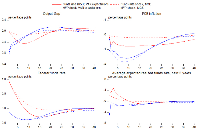
Impulse response functions to funds rate and multi-factor productivity shocks
Impulse response functions present the joint evolution of the model's variables in response to some well-defined exogenous shock. They are a common tool for analyzing the dynamic properties of complex models like FRB/US, in which the dynamics of key variables are highly interdependent.10  Figure 1 presents impulse responses of the output gap, inflation, and the federal funds rate to two different shocks, an exogenous increase in the federal funds rate of 1 percentage point, and an exogenous, permanent increase in multi-factor productivity of 1 percent. The figure also illustrates the two expectations assumptions of the model introduced above, VAR-based expectations (the solid lines) and model-consistent expectations (the dashed lines). The impulse responses are computed assuming that the federal funds rate is set according to a simple rule originally presented in Taylor (1999), modified to allow for inertial behavior.11 

Figure 1: Impulse Responses to Funds Rate and MFP Shocks VAR Expectations vs Model-Consistent Expectations
Figure 1 shows forty quarters of impulse responses.  In the case of the funds rate shock, the funds rate initially rises 1 percentage point and then gradually returns to baseline.  The return is somewhat more rapid under VAR expectations than under model-consistent expectations.  The output gap is below baseline for five or six years, with a maximum decline of 0.4 percentage point under VAR expectations and 0.1 percentage point under MCE.  Inflation is below baseline by as much as 0.08 percentage point under VAR expectations and 0.02 percentage point under MCE.  The weighted average of the expected real funds rate over the next five years is above baseline for two or three years, with a maximum increase of 0.5 percentage point under VAR expectations and 0.2 percentage point under MCE. 
In the case of the MFP shock, the impulse responses under each expectations assumption are generally similar.  The output gap returns to baseline after three to four years, after initially falling 0.8 percentage point.  Inflation initially declines 0.2 percentage point and returns to baseline more slowly than does the output gap.  The federal funds rate falls by as much as 0.4 percentage point.

The responses of the output gap and inflation (shown in the upper two panels) to an increase in the federal funds rate of initially 1 percentage point are qualitatively similar to results found in the VAR literature (for example, Boivin et al., 2011) and in DSGE models (for example, Smets and Wouters, 2007). The size of the FRB/US inflation response is relatively small, however, reflecting the estimation of its price-wage sector over the period of low and stable inflation since the mid-1980s. As indicated by the solid and dashed lines, the magnitude of the responses depends on the manner in which expectations are assumed to be formed. This is not surprising: Expectations are important in the structure of FRB/US, and the two expectations approaches are based on views of the relationships among macro variables that are not identical. One specific difference in this area is the degree of inertia attributed to movements in the federal funds rate. The estimated funds rate equation that is part of the VAR-based expectations mechanism has more inertia than the Taylor-type policy rule used in FRB/US itself for these simulations. As a result, the initial interest rate increase is anticipated to be more persistent under VAR-based expectations than under model-consistent expectations (lower right panel, shown in real terms). Through its effect on real long-term interest rates, this difference causes the output gap and inflation to decline substantially more in the VAR-based case.12 

The responses of output and inflation to a permanent increase in multi-factor productivity (MFP) are also in general accordance with estimates from the VAR literature of the effects of technology shocks (see for example Altig et al., 2010), including the more rapid decline in inflation compared to a funds rate shock. In a model with sticky prices and wages, the level of actual output only gradually approaches the new, permanently higher level of potential output, so that the output gap initially declines. In response to the decline in the output gap and inflation, the federal funds rate temporarily falls below its baseline value.

Stochastic simulations
As a second illustration of the use of the model, figure 2 presents intervals around an illustrative baseline into which 70 and 90 percent of the simulated values of the variables fall. Because of the nonlinear structure of FRB/US, closed-form solutions for the unconditional variance of the endogenous variables at different projection horizons do not exist. To compute the intervals reported in the figure, the model with VAR-based expectations is simulated 1000 times, drawing at random from the series of historical equation residuals.13 

Figure 2: Stochastic Simulations (70 and 90 percent bands)
Figure 2 shows 70 and 90 percent bands for a simulation period that starts in 2014q1 and ends after five years, in 2018q4.  The following results obtain at the end of the third year, in 2016q4.  For the unemployment rate, the baseline value is 5.4 percent, the limits of the 70 percent band are 3.8 and 7.0, and the limits of the 90 percent band are 3.0 and 7.7.  For the federal funds rate, the baseline value is 2.25 percent, the limits of the 70 percent band are 0.9 to 4.0, and the limit of the 90 percent band are 0.25 (the effective zero bound) to 4.9.  For four-quarter core PCE inflation, the baseline value is 1.9 percent, the limits of the 70 percent band are 1.1 to 2.9, and the limits of the 90 percent band are 0.6 to 3.6.  For four-quarter real GDP growth, the baseline value is 2.75 percent, the limits of the 70 percent band are 1.0 to 4.7, and the limits of the 90 percent band are -0.2 to 5.7.

Contents of the Web Page
The main FRB/US web page provides access to the following material:

  • FRB/US model package: This contains the package of code needed to simulate FRB/US using the EViews software (the EViews software itself needs to be previously installed by the user). It includes files containing model equations and parameters as well as a database. The database will be updated periodically. The model files themselves will be updated occasionally, usually once a year, reflecting specification changes or re-estimation of model equations. The package also contains the two sample programs described above.
  • FRB/US supply-side model: This provides the code and data used for estimating a state-space model similar to that developed in Fleischman and Roberts (2011) on which the FRB/US specification of potential output and its components is based.
  • RE solver package: For users who are primarily interested in the solution algorithms for solving linear and nonlinear models under MCE, this provides the library of EViews code that implements these algorithms, as well as sample programs and specific documentation.
  • Research papers and documentation: This page features links to articles that use the FRB/US model as well as to published and unpublished documentation of the FRB/US model.


1. Flint Brayton is a contractor, Thomas Laubach is Associate Director, and David Reifschneider is Deputy Director (retired), all in the Division of Research and Statistics. The authors would like to thank Michael Palumbo, John Roberts, and David Wilcox for helpful comments. Return to text

2. The Board's website also contains a new page devoted to EDO, which is another model of the U.S. economy that is used by Board staff. Return to text

3. The general design of FRB/US shares many features with the "New Neoclassical Synthesis" class of models (Goodfriend and King, 1997). Return to text

4. Detailed documentation of the original specification of FRB/US can be found in Brayton and Tinsley (1996), and properties of early versions of the model are discussed in Brayton et al. (1997a,b) and Reifschneider et al. (1999). Since then, the model has undergone a number of changes, including modifying the price-wage sector to shift from a price index for domestic absorption and P&C hourly compensation as the main price and wage measures to the core PCE price index and ECI hourly compensation; modifying the production function in a number of ways, including the use of BLS capital services and the estimation of trend MFP as a stochastic process; the adoption of chain aggregation; multiple specification changes to the export/import equations that over time have significantly altered their short-run dynamics and long-run price/income elasticities; a more elaborate accounting of net foreign investment income and the net foreign asset position of the US; the introduction of house prices to the wealth accounting structure; and the introduction of government debt-stabilization rules. For more recent documentation of some of the model's sectors, the reader is referred to the documentation section of the web page as well as the HTML documentation of the model's individual equations that is part of the FRB/US download package. Return to text

5. FRB/US currently contains about 60 stochastic equations, 320 identities, and 125 exogenous variables. Return to text

6. The main structural price and wage equations are estimated simultaneously in the same small model. See the note "A New FRB/US Price-Wage Sector" by Brayton (2013) in the documentation section of the web page. Return to text

7. For a detailed discussion of the assumptions with which expectations are modeled in FRB/US, see Brayton et al. (1997a). Return to text

8. Recent developments of numerical algorithms have greatly increased the speed with which large-scale nonlinear MCE models can be solved. MCE simulations of FRB/US are executed in EViews using the algorithms described in Brayton (2011). More information on these algorithms is available in the "RE Solver Package" section of the FRB/US web pages. Return to text

9. SIGMA: Erceg et al. (2006). EDO: Edge et al. (2008). Return to text

10. The program pings.prg included in the FRB/US package computes impulse responses to six such shocks and plots the responses of two key variables, inflation and the output gap, to these shocks. Return to text

11. Specifically, let i_tdenote the nominal federal funds rate, r the steady-state real short-term interest rate,  \pi_tthe four-quarter rate of inflation,  \overline{\pi} the inflation objective, and  x_t the output gap. The policy rule used in the simulations is  i_t = \rho_ii_{t-1} + (1 - \rho_i)(r + \pi_t + \phi_\pi(\pi_t - \overline{\pi}) + \phi_xx_t) + \varepsilon_t, with an interest smoothing parameter  \rho_iof 0.85, and the values for  \phi_\pi and  \phi_xof 0.5 and 1, respectively. Return to text

12. If the expectations error about the policy rule made by agents under VAR-based expectations is eliminated by re-running both the VAR and MCE simulations using the estimated average historical funds rate rule embedded in the VAR, rather than the simple inertial rule described in footnote 11, then outcomes under MCE and VAR-based expectations become quite similar. Return to text

13. The program stochsim.prg included in the FRB/US package provides code for stochastic simulations of the model around the illustrative long baseline projection given in the database longbase.db, which is also included in the package. The baseline outlook for the unemployment rate, real GDP growth, and inflation for the years 2014 through 2016 follows the midpoints of the central tendencies of the projections of Federal Open Market Committee (FOMC) participants submitted in conjunction with the March 2014 FOMC meeting. The outlook for the federal funds rate follows the median projection of FOMC participants. All other aspects of the projections included in the database should not be construed as reflecting the views of the FOMC or any of its participants. Return to text


References

Altig, David, Lawrence Christiano, Martin Eichenbaum, and Jesper Linde, 2010. "Firm-Specific Capital, Nominal Rigidities and the Business Cycle." Review of Economic Dynamics 14, 225-247.

Boivin, Jean, Michael Kiley, and Frederic Mishkin, 2011. "How Has the Monetary Transmission Mechanism Evolved Over Time?" In Benjamin Friedman and Michael Woodford, eds., Handbook of Monetary Economics Vol. 3 (Elsevier), pp. 369-422.

Brayton, Flint, 2011. "Two Practical Algorithms for Solving Rational Expectations Models." Finance and Economics Discussion Series 2011-44, Federal Reserve Board.

Brayton, Flint, and Peter Tinsley, 1996. "A Guide to FRB/US: A Macroeconomic Model of the United States." Finance and Economics Discussion Series 1996-42, Federal Reserve Board.

Brayton, Flint, Eileen Mauskopf, David Reifschneider, Peter Tinsley, and John Williams, 1997a. "The Role of Expectations in the FRB/US Macroeconomic Model." Federal Reserve Bulletin, April, 227-245.

Brayton, Flint, Andrew Levin, Ralph Tryon, and John Williams, 1997b. "The Evolution of Macro Models at the Federal Reserve Board." Carnegie-Rochester Conference Series on Public Policy, Vol. 47, 43-81.

Carroll, Christopher A. (2001), "A Theory of the Consumption Function, With and Without Liquidity Constraints," Journal of Economic Perspectives 15(3), pp. 23-46.

Cogley, Timothy, and Argia Sbordone, 2008. "Trend Inflation, Indexation, and Inflation Persistence in the New Keynesian Phillips Curve." American Economic Review 98, 2101-2126.

Edge, Rochelle, Michael Kiley, and Jean-Phillipe Laforte, 2008. "Natural Rate Measures in an Estimated DSGE Model of the U.S. Economy." Journal of Economic Dynamics and Control 32, pp. 2512-2535.

Erceg, Christopher, Luca Guerrieri, and Christopher Gust, 2006. "SIGMA: A New Open Economy Model for Policy Analysis." International Journal for Central Banking 2, pp. 1-50.

Fleischman, Charles, and John Roberts, 2011. "From Many Series, One Cycle: Improved Estimates of the Business Cycle from a Multivariate Unobserved Components Model." Finance and Economics Discussion Series 2011-46, Federal Reserve Board.

Goodfriend, Marvin, and Robert King, 1997. "The New Neoclassical Synthesis and the Role of Monetary Policy." NBER Macroeconomics Annual 12, 231-283.

Reifschneider, David, Robert Tetlow, and John Williams, 1999. "Aggregate Disturbances, Monetary Policy, and the Macroeconomy: The FRB/US Perspective." Federal Reserve Bulletin, January, 1-19.

Smets, Frank, and Rafael Wouters, 2007. "Shocks and Frictions in US Business Cycles: A Bayesian DSGE Approach." American Economic Review 97, 586-606.

Taylor, John, 1999. "A Historical Analysis of Monetary Policy Rules." In John Taylor, ed., Monetary Policy Rules (Chicago: University of Chicago Press), pp. 319-41.

Tinsley, Peter, 2002. "Rational Error Correction." Computational Economics 19, 197-225.

Resources

Please cite as:

Brayton, Flint, Thomas Laubach, and David Reifschneider (2014). "The FRB/US Model: A Tool for Macroeconomic Policy Analysis," FEDS Notes. Washington: Board of Governors of the Federal Reserve System, April 03, 2014. https://doi.org/10.17016/2380-7172.0012

Disclaimer: FEDS Notes are articles in which Board economists offer their own views and present analysis on a range of topics in economics and finance. These articles are shorter and less technically oriented than FEDS Working Papers.

Search Working Papers


Skip stay connected section
Last update: April 3, 2014