
FEDS Notes
 Print
PrintJune 29, 2016
Findings on Relative Deprivation from the Survey of Household Economics and Decisionmaking
Sam Dodini
The Federal Reserve's Survey of Household Economics and Decisionmaking (SHED) contains questions designed to ascertain overall economic well-being and fragility, which can be used to gauge both the perceptions individuals have about their own economic status and an approximation of their actual financial health.1 The SHED contains valuable information that can be used to explore how the well-being of others in their community may impact an individual's assessment of their own well-being and their choices.
Typical measures of financial well-being often focus on income distributional statistics such as one's income or wealth level. Under the standard consumer utility framework, income is important for well-being by determining the budget constraint and impacting the level of consumption that one can afford. Since well-being is based solely on one's own income and consumption, well-being will have no direct relation to the income or consumption of others.
However, under theories first developed by Duesenberry (1949), individual utility may not depend on consumption subject to absolute income constraints and prices, but also upon relative income. As one's relative income falls, their level of relative deprivation increases, as does their disutility, even if their own income or consumption remains unchanged.
Under this theory of relative deprivation, not only do quantities consumed matter to utility, but in order to combat the disutility of lower relative income, individuals reallocate their income toward consumption goods designed to keep up with their higher-income peers. Spending is particularly focused on "positional goods"--a term first coined by Hirsch (1977) to mean goods that represent more expensive outward signals of success and whose utility comes from exclusivity. Examples include expensive cars, the newest electronic gadgets, or fashionable clothing. The prediction of relative deprivation theory is that lower relative income households attempt to maintain a higher quality lifestyle in order to keep up with higher relative income households in a kind of expenditure arms race (the proverbial "Keeping up with the Joneses"), as discussed extensively by Frank (2007). Based on relative deprivation theory, increases (decreases) in inequality can reduce (increase) individual well-being beyond that which would be expected from changes in any individual's own income.
While relative deprivation is one way in which inequality levels can impact individual well-being, it is not the only avenue by which an impact may occur. To the extent that inequality increases the cost of living due to competition for scarce resources--which often occur simultaneously with the economic growth of cities and gentrification--the higher prices will reduce the consumption possibility frontier for an individual with a given level of income2. As an example, Glaeser, et al (2012), relate their findings that city centers with more poverty, coupled with higher-income periphery areas, saw the greatest house price growth from 1996-2006 as the central cities revitalized (and local inequality increased), which may have negatively affected the well-being of those lower-income residence who occupied those city centers.
In this case, the relationship between consumption and well-being from classical economic theory will adequately predict lower well-being for those in high-cost areas due to price effects without relying on this relative deprivation explanation. Local prices are key to understanding the amount of weight to place upon relative deprivation theory vis-à-vis price theory.
For this analysis, I focus on two main questions in the SHED related to this theory of relative deprivation. Respondents are asked how they perceive themselves to be faring financially, ranging from "Finding it difficult to get by" to "Living comfortably" and also about their expenses relative to their income as a measure of savings. If relative deprivation leads to overspending or viewing one's household as financially worse off than others, we would expect those with lower relative incomes to report lower levels of financial health and savings. In making comparisons that may affect one's perceptions of relative economic standing, individuals depend heavily upon their social interactions and their immediate environment. They draw from their experiences in communities, not across countries. For this reason, analyses that attempt to fully explore these issues should examine them at the local rather than national level.
The restricted use version of the 2014 SHED data contain demographic information measuring age, income, education, household size, marital status, and race/ethnicity along with the ZIP code information of each of the approximately 5,800 survey respondents across more than 4,600 ZIP codes. Using the ZIP code information of the respondents, we can compare the reported income of the respondent to the ZIP code level 5-year estimates of income as measured by the American Community Survey (ACS) in order to measure how one's own income compares to the incomes of those above them in the income distribution.
Measuring Relative Deprivation
Gini-based indexes of relative deprivation account for the concentration of income as well as the proportion of the income distribution above a household of interest (e.g. Yitzhaki, 1979), i.e. the distribution of income. The SHED, however, reports household-level incomes and other important facets of well-being. In terms of individual knowledge of their own position in a community, I argue that households are unlikely to readily perceive the distribution of income that surrounds them as much as they perceive the difference in the levels of income between themselves and those that are relatively well off in the community.3 Thompson (2016) makes a similar argument that Gini measurements do not adequately capture changes at the top of the income distribution nor address the true relative income of those at the middle and bottom. To measure this perception in the SHED, I construct a metric of each household's income as a percentage of the 90th percentile income in their ZIP code. The lower the percentage below one, the more relative deprivation applies to the respondent and/or their household. I adjust the measure for those whose income is greater than the 90th percentile to 1, as they face no relative deprivation in connection to the reference group.4
A Snapshot of Current Well-Being
First, I examine the relationship between both absolute and relative income and self-reported financial well-being in the SHED. Figure 1 shows the straightforward relationship between stated living conditions and absolute income. The results are exactly what we would expect: those in lower income buckets are more likely to respond that they are finding it difficult to get by.
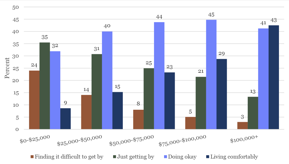 |
Source: 2014 Survey of Household Economics and Decisionmaking (SHED)
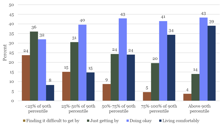 |
Source: 2014 Survey of Household Economics and Decisionmaking (SHED) and American Community Survey (ACS)
Figure 2 shows a similar relationship between financial well-being and relative income. Among those whose income is less than 25 percent the 90th percentile value, only eight percent responded that they are "living comfortably" compared to 34 percent of those whose income is 75 to 100 percent of the 90th percentile income. In the lowest category, 24 percent of those whose incomes are less than 25 percent of the 90th percentile say they are "finding it difficult to get by", compared to 4-5 percent of those whose incomes are near or above the 90th percentile.
The similarities between Figures 1 and 2 underscore the need to adequately control for absolute income when examining the effects of relative income. I use an ordered probit regression model to isolate these effects. I also include other controls that may influence household perceptions of well-being and financial behavior. These are personal demographics that reflect life cycle and preferences, i.e. ethnicity, age, and education; the household characteristics of household size and marital status; employment status; and the ZIP-level considerations of average household size and cost of living measured by median house value. Table 1 shows the incremental results of including these controls.
| Overall Financial Well-Being | Income Greater than Expenses (Savings) | |||
|---|---|---|---|---|
| (1) | (2) | (3) | (4) | |
| Relative Income as % of 90th Percentile | 0.0783 (0.149) |
-0.00133 (0.188) |
0.527*** (0.175) |
0.264 (0.226) |
| Relative Income as % of 90th Percentile Squared | 0.141 (0.0914) |
0.144 (0.0930) |
0.125 (0.108) |
0.151 (0.108) |
| Age 30-44 | -0.175*** (0.0578) |
-0.291*** (0.0605) |
-0.105 (0.0735) |
-0.161** (0.0767) |
| Age 45-59 | -0.0851 (0.0581) |
-0.256*** (0.0637) |
0.0512 (0.0709) |
-0.0612 (0.0776) |
| Age 60+ | 0.456*** (0.0569) |
0.273*** (0.0715) |
0.173*** (0.0669) |
0.0699 (0.0829) |
| Black, Non-Hispanic | -0.153** (0.0611) |
-0.112* (0.0631) |
-0.167** (0.0769) |
-0.161** (0.0778) |
| Bachelor's degree or higher | 0.345*** (0.0751) |
0.282*** (0.0765) |
0.239*** (0.0916) |
0.150 (0.0930) |
| Divorced/Widowed/Separated/Living with Partner | -0.265*** (0.0480) |
-0.180*** (0.0588) |
||
| Never Married | -0.238*** (0.0564) |
-0.0698 (0.0700) |
||
| Household Size | -0.0811*** (0.0154) |
-0.0967*** (0.0210) |
||
| Not Employed | -0.0524 (0.0467) |
-0.113** (0.0551) |
||
| Average Household Size (ZIP) | -0.0890* (0.0460) |
-0.0545 (0.0603) |
||
| Log Median House Value (ZIP) | -0.0277 (0.0420) |
-0.107** (0.0533) |
||
| Observations | 5,815 | 5,801 | 5,779 | 5,767 |
| Personal Controls | Yes | Yes | Yes | Yes |
| Household, Work Status, ZIP Characteristics | No | Yes | No | Yes |
| Log Likelihood | -6806 | -6746 | -3711 | -3665 |
| Pseudo R2 | 0.0903 | 0.0966 | 0.0535 | 0.0635 |
Note: The regression includes unreported categories for race/ethnicity of Hispanic, Other/Non-Hispanic, 2+ Non-Hispanic and for education groups of high school and some college (no degree) and work status of not employed, each of which are not statistically significant. Absolute income is controlled by including categorical buckets so as to allow for nonlinear effects of absolute income.
Source: Author's calculations of SHED data.
These regressions control for absolute income. However, other characteristics are also important factors in what social comparisons people may draw and the financial decisions they may make. The age of the respondents in particular plays an important role because individual incomes vary predictably over the life cycle. The education of the respondent is also important because higher levels of education are correlated with preferences for patience and financial literacy, which factor into financial well-being. In addition, nominal dollars of income do not buy someone the same level of consumption across different locations. For example, housing and other expenses are far higher in Manhattan than they are in Ithaca, NY. Someone making $60,000 per year in Manhattan is not necessarily better off than someone making $58,000 in Ithaca. In order to effectively compare these individuals to each other and to others within their cities, we must control for the cost of living. While a measure of local consumer prices is not directly available, house prices are available, which constitute a major contributor to local cost of living calculations.5 Columns 2 and 4 include the log of median house price as a proxy for local costs.
In all specifications, there is no statistically significant relationship between relative deprivation and self-reported financial well-being (columns 1-2).6 This may be due to the fact that there are only four response categories that may miss more narrow changes in perception or may reflect the idea that these differences may simply not enter their financial "big picture" but may play a role in their day-to-day decisions. More concrete measures of financial health would help us understand what other factors may be related. If relative deprivation had a negative association with utility or self-perception, we would expect to see a negative relationship. These results are inconsistent with the positional goods theory of relative deprivation.
Concrete Financial Status
In addition to asking about the way individuals perceive their overall financial well-being, the SHED also asks questions designed to understand the financial health of the household in a more concrete way.
To understand overall and emergency savings, the SHED asks respondents how their spending compares to their income over the previous 12 months. Prolonged household budget deficits can lead to the accumulation of debt, increased stress and economic fragility, and limit upward mobility. In addition, if prices are driven upward by the spending of high-income households, or if concerns about relative position in the community drive households to spend more on positional, nonessential, or other goods, they are less likely to have money set aside for emergency expenses. Therefore, the relationship between savings and relative deprivation can inform the overarching consumption decisions of these individuals. In a similar vein, using payment to income ratios as a measure of debt and state-level income distributions in the Survey of Consumer Finances (SCF), Thompson (2016) finds that as the income of the state's 95th percentile increase relative to the rest of the distribution, payment to income ratios for those in the middle of the distribution also increase. These effects are not observed in the bottom of the distribution. As with other studies, state-level distributional analyses leave considerable room for heterogeneity in cost within states and within metro areas, which this analysis seeks to address.
Similar to the ordered probit regression discussed above, I also run a probit analysis of the binary outcome of whether or not a household's income was greater than their expenses, or in other words, whether or not the household set aside any real savings. Table 1, columns 3-4 outline the results of interest for each specification.
Column 3 indicates that, even after controlling for absolute income, those who are further away from the 90th percentile income are less likely than those who are closer to the 90th percentile to report that their income was greater than their expenditures, a relationship similar to Thompson's results. This is consistent with the sociological positional goods argument. Taken alone, this would suggest that relative deprivation is resulting in an increase in spending relative to income as individuals are attempting to keep up with the "Joneses." However, Column 4 shows that this relationship between relative income and spending beyond one's means declines and becomes statistically indistinguishable from zero upon inclusion of log median house value in the regression. This indicates that cost of living is highly connected to how relative deprivation relates to savings.7 Column 4 results are inconsistent with relative deprivation theory.
These results cast some doubt on the "Keeping up with the Joneses" and positional goods explanation of consumption. After controlling for absolute income, other important demographic covariates, and cost of living, those who face larger amounts of relative deprivation are not necessarily less likely to set aside savings over the course of a year. Rather, those with lower relative income appear to have lower levels of savings because they live in areas with higher prices and not necessarily because they are spending more in reaction to the higher-income "Joneses". Controlling for cost of living in these analyses is key to understanding the possible effects of relative deprivation on well-being independent of price effects.
Conclusion
Taken together, these analyses suggest that relative deprivation is weakly associated with lower marginal savings, but these influences may simply be manifestations of the effects of costs. Relative deprivation does not appear to be a large enough factor to shift individual perceptions of their overall financial well-being. Further analyses may utilize more measures of relative deprivation to investigate other components of the relationship between well-being and relative deprivation such as the percentage of income saved, their perceptions of mobility, and their preferences for work.
References
Cruces, Guillermo, Ricardo Perez-Truglia, and Martin Tetaz. 2013. Biased Perceptions of Income Distribution and Preferences for Redistribution: Evidence from a Survey Experiment. Journal of Public Economics 98: 100-112.
Duesenberry, J.S. 1949. Income, Saving and the Theory of Consumer Behavior. Harvard University Press, Cambridge, Mass.
Frank, Robert H. 2007. Falling Behind: How Rising Inequality Harms the Middle Class. University of California Press.
Glaeser, Edward L., Joshua Gottlieb, and Kristina Tobio. 2012. Housing Booms and City Centers. American Economic Review: Papers & Proceedings 102(3): 127-133.
Hirsch, Fred. 1977. Social Limits to Growth. Routledge & Kegan Paul Ltd.
Thompson, Jeffrey. 2016. Do Rising Top Incomes Lead to Increased Borrowing in the Rest of the Distribution? Finance and Economics Discussion Series 2016-046. Board of Governors of the Federal Reserve System.
Yitzhaki, Shlomo. 1979. Relative Deprivation and the Gini Coefficient. The Quarterly Journal of Economics 93(2): 321-324.
1. For the full report of survey results from each year, the instrument, and technical notes, see https://www.federalreserve.gov/communitydev/shed.htm. Return to text
2. For this reason, national income distributional statistics routinely adjust for cost of living. However, for local analyses, changes in cost of living will still play a role to the extent that local cost trends diverge from national averages. Return to text
3. Research from Argentina suggests that individuals are poor judges of their place in and the shape of the income distribution (Cruces, Perez-Truglia, and Tetaz, 2013). However, individuals are able to see positional goods or conspicuous consumption from which to infer ostensible differences in income levels. Return to text
4. I also compare these values using the 75th, 85th, and 95th percentiles for robustness. Return to text
5. BEA produces a regional price parity index. The correlation between median house price and this price parity for all goods at the state level is very high at 0.91. For more information, see http://www.bea.gov/newsreleases/regional/rpp/rpp_newsrelease.htm. Return to text
6. This also holds when comparing the 75th and 85th percentile levels to household income. However, distance from the 95th percentile appears to give mixed results. Return to text
7. Comparing these results to regressions using the gap between the household's income and the 75th, 85th, and 95th percentiles yields similar results, although column 3 results are not statistically significant for the 95th percentile. Return to text
Please cite this note as:
Dodini, Samuel (2016). "Findings on Relative Deprivation from the Survey of Household Economics and Decisionmaking," FEDS Notes. Washington: Board of Governors of the Federal Reserve System, June 29, 2016, http://dx.doi.org/10.17016/2380-7172.1791.
Disclaimer: FEDS Notes are articles in which Board economists offer their own views and present analysis on a range of topics in economics and finance. These articles are shorter and less technically oriented than FEDS Working Papers.
