IFDP Notes
June 15, 2018
Monitoring the World Economy: A Global Conditions Index1
Pablo Cuba-Borda, Alexander Mechanick, and Andrea Raffo
1. Introduction
The global financial crisis reminded academics and policymakers that the world economy is highly integrated. Between 2008 and 2009, world manufacturing production fell 15 percent, world trade collapsed nearly 30 percent, and unemployment rates jumped almost everywhere. Many economies experienced their deepest recession since the Great Depression. These events generated renewed efforts in the development of measures of global business conditions. In this note we present a Global Conditions Index (GCI), a real-time measure of the health of the global economy constructed using a small set of world economic variables. The GCI can be used to produce nowcast estimates of world GDP growth or to assess the likelihood of turning points in global economic activity. We provide one example that uses the GCI and a measure of financial stress to estimate recession probabilities in the world economy using a machine learning algorithm.
2. Methodology
The GCI results from the estimation of a parsimonious statistical model that summarizes the evolution of $$n$$ observed world economic variables (of possibly mixed frequencies), $$Y_{t}$$, as a linear function of a single unobserved common factor, $$X_{t}$$:
where $$A$$ is a nx1 vector, $$\eta_{t}\lesssim iid N(0,\sigma), \nu_{t}\lesssim N(0,I), and E(\nu_{t}, \eta_{t+s}) = 0$$ for all $$s$$. These assumptions allow to estimate the system of equations (1)-(2) using standard Kalman filter techniques and to extract the unobserved component $$X$$, which is our measured GCI, as well as estimates of its persistence $$(\rho)$$.2 A real-time forecast of the GCI can then be obtained according to the formula3
where the first term represents past values of the GCI itself and the second term is an update that incorporates new information about indicators contained in $$Y_{t}$$ using estimates for $$A$$ through the Kalman gain factor $$k$$.
The $$Y_{t}$$ variables include three monthly indicators, namely world industrial production (IP) growth, world retail sales (RS) growth, and the new export order component of the global Purchasing Managers Index (PMI), as well as quarterly world GDP growth.4 Hence, in this application n = 4. The estimation sample covers the period 1970M9-2017M12. The estimation removes time-varying trends--because of demographic factors, for example--using a nonparametric low-pass filter.5 Thus, the GCI can be interpreted as an indicator of world business cycle conditions.
Table 1 presents estimates of the econometric model (1)-(2) for the global economy. All estimated parameters of the coefficients in A are statistically significant and of the expected sign. All four macroeconomic series respond positively to the GCI, reflecting a positive co-movement with underlying business cycle conditions. The estimated autocorrelation coefficient $$(\rho)$$ is 0.86, pointing to a significant degree of persistence in global business conditions.
Table 1: Estimation results
| Variable | Loading on GCI |
|---|---|
| Industrial Production (IP) | 4.08*** (0.35) |
| New Export Orders (PMIs) | 1.66*** (0.25) |
| Retail Sales (RS) | 2.03*** (0.21) |
| GDP | 0.52*** (0.04) |
| Persistence of GCI factor | |
| ρ | 0.86*** (0.03) |
*** denotes 1% significance level; standard errors in parenthesis.
Given these estimates and equation (3), one can compute the contribution of each variable to changes in the GCI. IP and RS explain more than half of the GCI forecast error variance, whereas the PMIs account for less than 20 percent of it. That said, the PMIs are available sooner than IP and RS, which allows us to produce preliminary forecasts of the GCI at the beginning of a given quarter. World GDP growth explains the remaining share of the GCI forecast error variance, but this variable provides information only at a quarterly frequency and is available with considerable delay. Hence, it cannot be used to produce real-time updates of the GCI.
As shown in Figure 1, the estimated GCI (red line) can be used to produce an estimated series of monthly world GDP growth (blue line). The GCI and monthly GDP growth track each other very well. Consistent with our interpretation of an indicator of global economic conditions, the GCI increases during world economic expansions, declines sharply at the onset of recessions, and remains close to its zero-mean during periods of average growth.
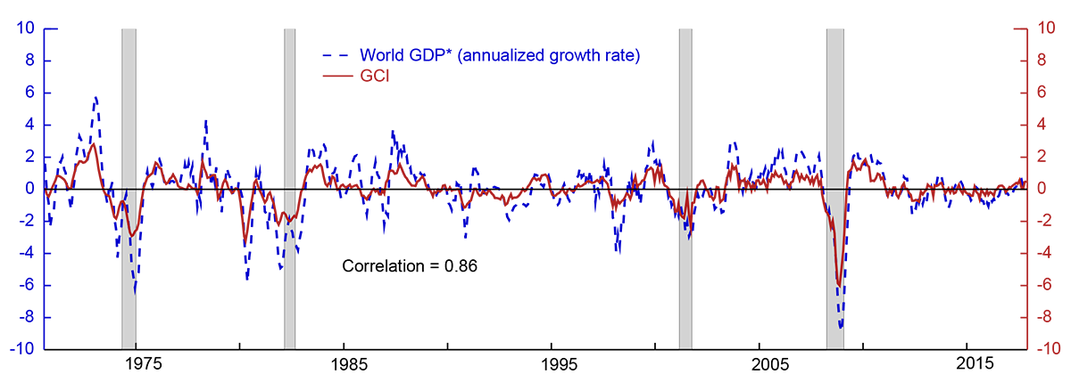
* For comparison world GDP growth is demeaned and expressed relative to its sample average growth rate of 3.7 percent.
Note: Shading indicates that countries representing 65% of foreign GDP are classified as in recession.
Source: Staff calculations.
The GCI can be used to produce real-time nowcast estimates of world GDP well before the release of the quarterly GDP data. As an illustrative example, Figure 2 presents nowcast estimates of world GDP growth obtained in the last month of the quarter using one month of IP data, two months of RS data, and three months of PMI data (blue dots). The real-time nowcast based on the GCI appears to track well the world GDP series and is available more than two months before the first release of official GDP data. And with PMIs typically available at the end of each month, the first nowcast of GDP growth in a given quarter can be produced up to four months in advance of the GDP release. Uncertainty about these very preliminary estimates, however, is generally very high.

3. World Recession Probability Estimates
The GCI can also provide useful information to detect turning points in world economic conditions. Consider an econometric model that specifies a relationship between indicators of economic and financial activity and recession outcomes:
where $$Z_{t\mid t+k}$$ is a world recession indicator that takes the value of 1 if the world economy is in recession in any month over the subsequent $$k$$ months, $$GCI_{t}$$ is the global condition index presented in the previous section, and $$EBP_{t}$$ is the excess bond premium series produced by Gilchrist and Zakrajšek (2012).6 The world recession indicator $$Z_{t\mid t+k}$$ is constructed using country-specific recession dates obtained from the Economic Cycle Research Institute (ECRI), which follows a methodology similar to that of the National Bureau of Economic Research to date recessions.7 In this analysis, a world recession occurs when countries representing about two-thirds of world GDP are classified as in recession.8 This procedure identifies four world recession episodes during our full sample period: June 1974 through March 1975, April 1982 through October 1982, April 2001 through November 2001, and April 2008 through May 2009. The unconditional probability of observing a world recession in any given month $$(k=0)$$ is 7 percent while the unconditional probability of observing a world recession over the subsequent 12 months is 16 percent. For comparison, the same statistics for the United States are 16 and 30 percent, respectively.
Figure 3 presents contemporaneous $$(k=0)$$ and one-year ahead $$(k=12)$$ recession probability estimates obtained from a nonparametric random-forest model. The random-forest methodology is appealing here as it does not require us to assume a functional relation among variables, thus resulting in a lower number of estimated false positives.9,10 World recession probability estimates line up well with the four events classified as world recessions using the information from the ECRI. In particular, estimates for one-year ahead recession probability rise well above the unconditional probability of observing a world recession (dashed line) several months before all the four recessions in the sample, pointing to a strong predictive power of turning points in world business cycles. There are, however, a few false signals--spikes in the estimates that reached the 50 percent level without an accompanying recessionary episode in the subsequent months. All told, both the contemporaneous and the one-year ahead recession probability estimates point to low risk of recession for the world economy as of March 2018.
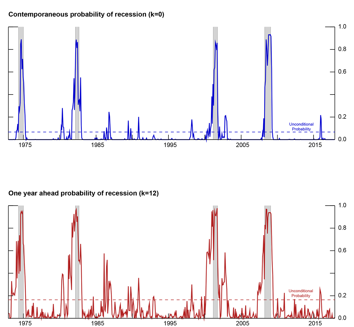
Note: Shading indicates that countries representing 65% of foreign GDP are classified as in recession.
Source: Staff calculations.
Figure 4 presents detailed estimation results for the world recession model in the form of a heat map. The two panels depict the recession probability associated with combinations of the GCI (x-axis) and the EBP (y-axis). As shown by the vertical bar to the right of each panel, blue cells indicate near-zero world recession probability estimates whereas yellow cells indicate near-unity recession probability estimates. The left panel corresponds to the contemporaneous recession probability $$(k=0)$$, whereas the right panel shows results for the probability of a recession taking place within the next year $$(k=12)$$.
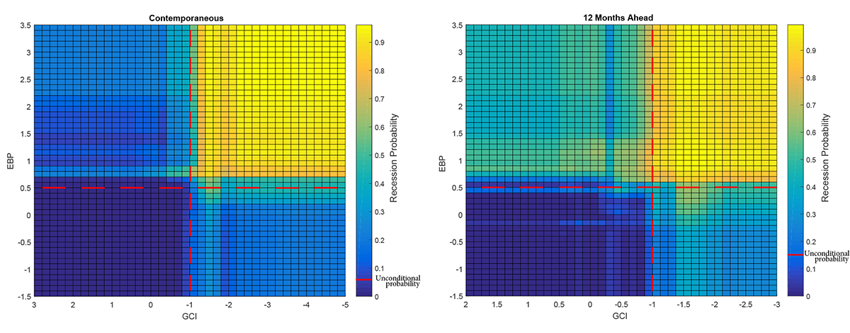
The heat map highlights the sensitivity of recession probability estimates to changes in the underlying economic and financial indicators. For instance, as depicted by the north-east quadrant delineated by the red dashed lines in Figure 4, when the GCI falls below -1.0 (reverse scale on the horizontal axis) and the EBP increases above 0.5 (vertical axis), estimates of a world recession probability over the next twelve months (right panel) increase sharply from their unconditional value of 16 percent to nearly 80 percent.
4. Conclusions
This note has presented the GCI, a new global economic index available in real-time and useful to monitor the evolution of global business conditions. The GCI is constructed using world GDP data and a small set of world economic variables (IP, RS, and the new exports order component of the PMIs) that are readily available. The GCI can be used to produce nowcast estimates of world GDP growth at monthly frequencies well before the release of official GDP data. It can also provide useful information to predict turning points in world business cycles and to produce world recession probability estimates. The methodology used to construct the GCI can be easily extended to produce similar indicators of economic activity for regional aggregates and for individual countries.
Appendix. Comparison of random forest and parametric estimates
Table 2 presents two statistical tests that support the accuracy of the random forest estimates in detecting world recessions relative to standard parametric estimates obtained from probit models. The first test is the receiver operating characteristic (ROC) discrimination index, which measures the ratio of true estimated positives to false estimated positives compared to a guess produced with a fair coin. A ROC discrimination index equal to 1 indicates that the estimated model predicts the outcomes perfectly while a ROC index less than 0 indicates that the model does worse than the random guess. The second test is Efron's pseudo $$R^{2}$$, a measure of the proportion of variance explained by the model.11 This indicator provides more information than the ROC measure as it weights not just false and true positives but the magnitude of the predicted error for each estimate. As shown in the table, random forest model performs extremely well both in absolute and in comparison with estimates obtained from probit models.
Table 2: Goodness of fit
| Contemporaneous | 12 Months Ahead | |
|---|---|---|
| ROC discrimination index | ||
| Random forest model | 0.99 | 0.96 |
| Probit model | 0.94 | 0.74 |
| Efron's pseudo r-squared | ||
| Random forest model | 0.74 | 0.65 |
| Probit model | 0.49 | 0.37 |
References
S. Boragan Aruoba & Francis X. Diebold, & Chiara Scotti (2009), "Real Time Measurement of Business Conditions," Journal of Business and Economic Statistics, 27, 417–427.
S. Borağan Aruoba & Francis X. Diebold & M. Ayhan Kose & Marco E. Terrones, (2011). "Globalization, the Business Cycle, and Macroeconomic Monitoring," NBER International Seminar on Macroeconomics, University of Chicago Press, vol. 7(1), pages 245 - 286.
Olivier Biau & Angela D´Elia (2011), "Euro Area GDP Forecast Using Large Survey Dataset - A Random Forest Approach" Euroindicators Working Paper, 2011/002.
Leo, Breiman (2001). "Random Forests", Machine Learning. 45 (1): 5–32
Jon Faust & Simon Gilchrist & Jonathan H. Wright & Egon Zakrajšsek, (2013). "Credit Spreads as Predictors of Real-Time Economic Activity: A Bayesian Model-Averaging Approach," The Review of Economics and Statistics, MIT Press, vol. 95(5), pages 1501-1519, December.
Giovanni Favara & Simon Gilchrist & Kurt Lewis & Egon Zakrajšek, (2016). "Recession Risk and the Excess Bond Premium," FEDS Notes. Board of Governors of the Federal Reserve System, April.
Simon Gilchrist & Benoît Mojon, (2014). "Credit Risk in the Euro Area," NBER Working Papers 20041, National Bureau of Economic Research, Inc.
Simon Gilchrist & Egon Zakrajsek, (2012). "Credit Spreads and Business Cycle Fluctuations," American Economic Review, American Economic Association, vol. 102(4), pages 1692-1720, June.
James Hamilton, (1995). Time Series Analysis. Princeton University Press.
Boris Iglewicz & David Hoaglin, (1993). "How to Detect and Handle Outliers", The ASQC Basic References in Quality Control: Statistical Techniques, Edward F. Mykytka, Editor.
Roberto S. Mariano & Yasutomo Murasawa, (2003). "A new coincident index of business cycles based on monthly and quarterly series," Journal of Applied Econometrics, John Wiley & Sons, Ltd., vol. 18(4), pages 427-443.
Silvia Miranda-Agrippino & Hélène Rey, (2015). "World Asset Markets and the Global Financial Cycle," NBER Working Papers 21722, National Bureau of Economic Research, Inc.
James H. Stock & Mark W. Watson, (1989). "New Indexes of Coincident and Leading Economic Indicators," NBER Chapters, in: NBER Macroeconomics Annual 1989, Volume 4, pages 351-409 National Bureau of Economic Research, Inc.
James H. Stock & Mark W. Watson, (2012). "Disentangling the Channels of the 2007-2009 Recession," NBER Working Papers 18094, National Bureau of Economic Research, Inc.
James H. Stock & Mark W. Watson, (2016). "Factor Models and Structural Vector Autoregressions in Macroeconomics". In Handbook of Macroeconomics, Vol. 2.
1. The views expressed herein are those of the authors and do not necessarily reflect those of the Board of Governors of the Federal Reserve System or its staff. Daniel Molon and Dawson Miller provided excellent research assistance. Return to text
2. In the spirit of Stock and Watson (1989), the methodology produces a single common factor Xt. Following Mariano and Murasawa (2003) and Aruoba, Diebold, and Scotti (2009), the methodology allows for mixed frequency observations. Return to text
3. See Hamilton (1994), page 380. Return to text
4. World IP, RS, and PMI are constructed from individual country data using time-varying GDP weights. We remove extreme observations following Iglewicz and Hoaglin (1993), as outliers can have a disproportionate effect on the estimates. Return to text
5. See Stock and Watson (2012, 2015) for details. Return to text
6. This measure captures risk compensation demanded by investors, after accounting for expected losses due to default, in the U.S. corporate debt market. Though calculated only for the U.S., the EBP fluctuates with measures of global risk aversion and is available for the same time period used in the estimation for our global conditions index. The EBP series is highly correlated with a corresponding series for the euro area presented in Gilchrist and Mojon (2014) and leads by a several months the series of global risk aversion proposed in Miranda-Agrippino and Rey (2015). Favara, Gilchrist, Lewis and Zakrajšek (2016) use the EBP to predict the probability of U.S. recessions using a probit regression model and provide monthly updates of the EBP and U.S. recession probabilities at: https://www.federalreserve.gov/econresdata/notes/feds-notes/2016/updating-the-recession-risk-and-the-excess-bond-premium-20161006.html Return to text
7. The ECRI database covers 22 countries that amount to 75 percent of World GDP as of 2014. The list of countries includes: United States, Canada, Mexico, Brazil, Germany, France, United Kingdom, Italy, Spain, Switzerland, Sweden, Austria, Russia, Japan, China, India, Korea, Australia, Taiwan, New Zealand, South Africa and Jordan. For the euro area, we obtained official dates from the Center for Economic Policy Research, but also coded as recessions the months associated with the growth slowdowns of 2001 and 2002. Return to text
8. The two-thirds threshold can be interpreted as a normalization as it determines the size of the unconditional probability of a world recession. It does not, however, have significant effects on the time series of the recession probability estimates. Return to text
9. Breiman (2001) first introduced this methodology. See Biau and D'Elia (2011) for an application to GDP forecasting. The random forest method consist in the production of large number of bootstrapped subsamples (500 in our analysis) of the full dataset that are combined in trees mapping values of the explanatory variables to recession probabilities via a machine learning algorithm. The final estimate is obtained by taking a simple average of the values produced by each tree. Return to text
10. The Appendix presents evidence in support of the random forest models compared to standard parametric models (e.g. probit). Return to text
11. Efron's pseudo R2 is the ratio of the sum of the squared residuals to the sum of squared differences of true values from the average value. While capturing the same idea, it differs from a standard R2 constructed from OLS regression estimates because the dependent variable in our model (recession indicator) is not continuous while the predicted value (the probability of recession) is. Return to text
Cuba-Borda, Pablo, Alexander Mechanick, and Andrea Raffo (2018). "Monitoring the World Economy: A Global Conditions Index," IFDP Notes. Washington: Board of Governors of the Federal Reserve System, June 2018., https://doi.org/10.17016/2573-2129.45.
Disclaimer: IFDP Notes are articles in which Board economists offer their own views and present analysis on a range of topics in economics and finance. These articles are shorter and less technically oriented than IFDP Working Papers.