Determining the Severity of Macroeconomic Stress Scenarios

Kapo Yuen
Federal Reserve Bank of New York

In the midst of the 2008 financial panic caused by the collapse of the subprime housing market, the U.S. government responded with unprecedented measures, including liquidity provision through various funding programs, debt and deposit guarantees and large-scale asset purchases. In February 2009, the U.S. banking supervisors conducted the first-ever system-wide stress test on 19 of the largest U.S. bank holding companies (BHCs), known as the Supervisory Capital Assessment Program (SCAP) (Federal Reserve 2009a). The stress test required these 19 BHCs to undergo simultaneous, forward-looking exercises designed to determine whether they would have adequate capital to sustain lending to the economy in the event of an unexpectedly adverse scenario. By conducting this SCAP exercise, the supervisors hoped that it would reduce uncertainty and restore confidence in the U.S. financial institutions. In their 2010 staff reports, Peristian, Morgan and Savino (2010), of the Federal Reserve Bank of New York, concluded that the SCAP might have helped to quell the financial panic by releasing vital information about the BHCs. They claimed, "While investors did not need supervisors to tell them which banks had capital deficiencies, they were surprised by the size of the capital gaps and they used that information to revalue banks."

Since conducting the SCAP in 2009, the Federal Reserve System has conducted annual stress tests on the U.S. banking system, called the Comprehensive Capital Analysis and Review (CCAR). Additionally, the Dodd-Frank Wall Street Reform and Consumer Protection Act requires the Federal Reserve Board to conduct annual stress tests of bank holding companies with total consolidated assets of U.S. $50 billion or more. In each CCAR, the Federal Reserve Board generates an adverse macroeconomic scenario (two adverse scenarios in 2013) and requires BHCs to submit at least one adverse scenario that is related to their own specific portfolios and risk profiles. While the 2013 instructions for CCAR indicate that the adverse scenario developed by the BHC must reflect "a severely adverse economic and financial market environment," it does not specify what should be the "appropriate severity" of an adverse scenario used for the capital planning. This chapter will discuss the severity of the supervisory adverse scenarios and provide a simple methodology to compare the severity of different adverse macroeconomic scenarios. In particular, the key questions we aim to answer are:

• how to measure the severity of a firm's BHC macro stress scenario;
• how severe the BHC stress scenario is when compared with the supervisory stress scenarios; and
• what implications can be drawn about the credibility of the BHC's stress scenario.

The U.S. Supervisory Stress Scenarios
As part of the Federal Reserve System's Comprehensive Capital Analysis and Review (CCAR), U.S. domiciled top-tier bank holding companies (BHCs) are required to submit comprehensive capital plans, including pro forma capital analyses, based on at least one BHC defined adverse scenario. The adverse scenario is described by quarterly trajectories for key macroeconomic variables (MVs) over the next nine quarters (or longer, as in 2013). In addition, the Federal Reserve generates its own supervisory stress scenarios so that firms are expected to apply both BHC and supervisory stress scenarios to all exposures to estimate potential losses under stressed operating conditions. Separately, firms with significant trading activity are asked to estimate a one-time potential trading-related market and counterparty credit losses under their own BHC scenarios and market stress scenarios provided by the supervisors.¹  For the supervisory stress scenarios, the Federal Reserve provides firms with global market shock components that are one-time, hypothetical shocks to a large set of risk factors. For the last two CCAR exercises, these shocks involved large and sudden changes in asset prices, rates, and CDS spreads that mirrored the severe market conditions in the second half of 2008.

Since CCAR is a comprehensive assessment of a firm's capital plan, the BHCs are asked to conduct an assessment of the expected uses and sources of capital over a planning horizon. In the 2009 SCAP, firms were asked to submit stress losses over the next two years, on a yearly basis. Since then, the planning horizon has changed to nine quarters. For the last three CCAR exercises, a BHC is asked to submit its pro forma, post-stress capital projections in its capital plan beginning with data as of September 30, and spans the nine-quarter planning horizon. The projections begin in the fourth quarter of the current year and conclude at the end of the fourth quarter two years forward. Hence, for defining BHC stress scenarios, firms are asked to project the movements of key macroeconomic variables over the planning horizon of nine quarters. Our analysis on determining the severity of macro stress scenarios is based on the movements of the macroeconomic variables in these nine quarters. As for determining the severity of the global market shock components for trading and counterparty credit losses, it will not be discussed in this chapter because it is a one-time shock and the evaluation will be on the movements of the market risk factors rather the macroeconomic variables.

In the 2011 CCAR, the Federal Reserve defined the stress supervisory scenario using nine macroeconomic variables: real GDP, Consumer Price Index (CPI), real disposable personal income, unemployment rate, three-month Treasury bill rate, 10-year Treasury bond rate, BBB corporate rate, Dow Jones Index and National House Price Index (Federal Reserve 2011a). In CCAR 2012, the number of macroeconomic variables that defined the supervisory stress scenario increased to 14. Besides the original nine variables, the added variables were nominal GDP growth, nominal disposable income growth, mortgage rate, Market Volatility Index and Commercial Real Estate Price Index (Federal Reserve 2011b). Additionally, there is another set of 12 international macroeconomic variables, three macroeconomic variables and four countries/ country blocks, included in the supervisory stress scenario. As for CCAR 2013, the Federal Reserve System uses the same set of variables to define the supervisory adverse scenario (Federal Reserve 2012) as in 2012. Since the BHCs are required to define their own adverse scenarios of "a severely adverse economic environment," one way to determine the "appropriate severity" of the BHCs' stress scenarios is to compare them with the supervisory adverse scenarios. Although it is stated that the BHC stress scenarios should reflect the BHC's unique vulnerabilities to factors that affect its exposures, activities and risks, by comparing the severity of the BHC's and supervisory stress scenarios we can determine whether the estimates of the losses are consistent with the relative severity of the stress scenarios. For example, if the BHC's own stress scenario is deter- mined to be more severe than the supervisory scenario, but the estimated losses from the supervisory scenario are larger, then we would need to examine the details of the stress loss estimation methodology to determine the causes of this inconsistency.

Aligning the U.S. Supervisory Stress Scenarios
Let us consider the two CCAR supervisory stress scenarios in 2011 and 2012 and the supervisory severely adverse scenario in 2013. By comparing the forecast of the macroeconomic variables over the next nine quarters, we will try to determine which scenarios are the most and least severe.

In general, comparing severity of stress scenarios is relative. That is, we can usually deduce with relative confidence that Scenario A is more severe than Scenario B, but it is much more challenging to quantify how much more severe is Scenario A over Scenario B. In other words, it is much more difficult to define a metric to measure the severity of a stress scenario. Later in this chapter, we will attempt to use a historical event as a reference to give some insights on the measurement of severity.

Before we begin to examine the three supervisory scenarios, we will make the following key assumptions.

• All scenarios start on the same quarter, Q3 2010, and the projections are over the nine quarters from Q4 2010 to Q4 2012. Hence the scenarios are compared by measuring the change over the nine quarters on the macroeconomic variables.
• The scenarios are compared on the set of common macroeconomic variables. For example, in 2012 and 2013, the Market Volatility Index is included in the supervisory stress scenario, but not in 2011, thus this variable is excluded. Therefore, the set of common macroeconomic variables for comparison are all the variables that are defined in the supervisory scenario of 2011 CCAR.

Of the nine macroeconomic variables, Real GDP, CPI, and Real Disposable Personal Income are expressed as growth rates in 2012 and 2013 (see table 5.1). To convert them back to Real GDP, CPI, and Real Disposable Personal Income, we use equation 5.1 to convert growth rates into actual values, and align all the starting values using the Q3 2010 actual values. For variables such as unemployment rate (UR), we first align all the starting values to be Q3 2010, then we use the percentage change over the period (equation 5.2) to convert the 2012 and 2013 projections to the projections with the same starting values. For example, the Real GDP Growth Rate (Real_GDPGR) is converted to Real GDP (Real_GDP) by the following equation:

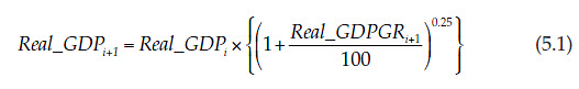
For other variables, the alignment is just the percentage change over the period,

 

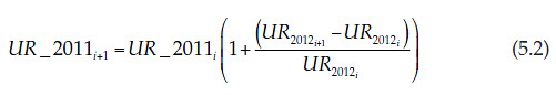
Table 5.1 The Federal Reserve supervisory adverse scenarios with nine quarters of projections

CCAR 2011 common variables	Q3 2010	Q4 2010	Q1 2011	Q2 2011	Q3 2011	Q4 2011	Q1 2012	Q2 2012	Q3 2012	Q4 2012
Real GDP	13,261	13,332	13,393	13,255	13,206	13,138	13,178	13,229	13,343	13,453
Real disposable personal income growth	10,237	10,271	10,299	10,318	10,236	10,179	10,081	10,054	10,047	10,066
Unemployment Rate	9.6	9.6	9.6	10.1	10.6	11	11.1	11	10.9	10.6
CPI	218	219	219.9	220.9	221.7	222.3	222.9	223.4	224	224.7
3-month Treasury yield	0.16	0.16	0.19	0.07	0.13	0.13	0.13	0.13	0.13	0.13
10-year Treasury yield	2.9	2.57	2.64	2.66	2.79	2.77	2.71	2.98	3.12	3.35
BBB corporate yield	5.07	4.69	4.86	5.88	6.26	6.46	6.16	6.27	6.22	6.25
Dow Jones Total Stock Market Index	11,947	12,069	11,822	9,116	8,809	8,716	10,682	11,083	11,498	11,930
National House Price Index	142	140	139	137	134	132	130	128	127	126

 

CCAR 2012 common variables	Q3 2011	Q4 2011	Q1 2012	Q2 2012	Q3 2012	Q4 2012	Q1 2013	Q2 2013	Q3 2013	Q4 2013
Real GDP growth	2.46	-4.84	-7.98	-4.23	-3.51	0	0.72	2.21	2.32	3.45
Real disposable personal income growth	-1.73	-6.02	-6.81	-4.29	-3.16	-0.57	0.74	1.66	2.69	2.27
Unemployment rate	9.09	9.68	10.58	11.4	12.16	12.76	13	13.05	12.96	12.76
CPI inflation rate	3.09	2.21	1.78	1.02	0.89	0.35	0.23	0.21	0.3	0.32
3-month Treasury yield	0.02	0.1	0.1	0.1	0.1	0.1	0.1	0.1	0.1	0.1
10-year Treasury yield	2.48	2.07	1.94	1.76	1.67	1.76	1.74	1.84	1.98	1.98
BBB corporate yield	4.87	5.65	6.83	6.81	6.75	6.45	6.07	5.83	5.74	5.51
Dow Jones Total Stock Market Index	11,771.86	9,501.48	7,576.38	7,089.87	5,705.55	5,668.34	6,082.47	6,384.32	7,084.65	7,618.89
National House Price Index	136.86	135.13	131.61	127.5	123.12	119.08	115.15	111.92	109.77	108.48

 

CCAR 2013 common variables	Q3 2012	Q4 2012	Q1 2013	Q2 2013	Q3 2013	Q4 2013	Q1 2014	Q2 2014	Q3 2014	Q4 2014
Real GDP growth	2	-3.5	-6.1	-4.4	-4.2	-1.2	0	2.2	2.6	3.8
Real disposable personal income growth	0.8	-3.8	-6.7	-4.6	-3.2	-1.5	0.8	0.9	2.5	2.8
Unemployment Rate	8.1	8.9	10	10.7	11.5	11.9	12	12.1	12	11.9
CPI inflation rate	2.3	1.8	1.4	1.1	1	0.3	1	0.9	0.7	0.6
3-month Treasury yield	0.1	0.1	0.1	0.1	0.1	0.1	0.1	0.1	0.1	0.1
10-year Treasury yield	1.6	1.4	1.2	1.2	1.2	1.2	1.2	1.5	1.7	1.9
BBB corporate yield	4.2	5.6	6.4	6.7	6.8	6.5	6.2	6.2	6	5.9
Dow Jones Total Stock Market Index	14997.8	12105.2	9652.6	9032.8	7269.1	7221.7	7749.3	8133.9	9026.1	9706.7
National House Price Index	143.4	141.6	137.9	133.6	129	124.7	120.6	117.2	115	113.6

After aligning the supervisory stress scenarios from CCAR 2011, 2012 and 2013, we also create an additional hypothetical stress scenario to illustrate how the severity of stress scenarios can be compared between the supervisory scenarios and a "BHC-developed" stress scenario, as part of the BHC's requirements under CCAR. Table 5.2 shows the three supervisory and the hypothetical scenarios as they are all aligned at Q3 2010. All the scenarios have the same set of macroeconomic variables and they are all aligned to the same value as of Q3 2010. Hence, by comparing the changes of the macroeconomic variables over the next nine quarters, we can examine the severity of each scenario relative the others.

Table 5.2 The macroeconomic variables with nine quarters of projections on the four scenarios

Scenario	CCAR common variables	Q3 2010	Q4 2010	Q1 2011	Q2 2011	Q3 2011	Q4 2011	Q1 2012	Q2 2012	Q3 2012	Q4 2012
2011	Real GDP	13,261	13,332	13,393	13,255	13,206	13,138	13,178	13,229	13,343	13,453
2012	Real GDP	13,261	13,097	12,828	12,690	12,577	12,577	12,599	12,668	12,741	12,849
2013	Real GDP	13,261	13,143	12,938	12,793	12,657	12,619	12,619	12,687	12,769	12,889
Hypothetical	Real GDP	13,261	12,690	12,690	12,690	12,690	12,690	12,690	12,690	12,690	12,690
2011	Real Disposable Personal Income	10,237	10,271	10,299	10,318	10,236	10,179	10,081	10,054	10,047	10,066
2012	Real Disposable Personal Income	10,237	10,079	9,903	9,795	9,717	9,703	9,721	9,761	9,826	9,881
2013	Real Disposable Personal Income	10,237	10,138	9,964	9,847	9,768	9,731	9,750	9,772	9,832	9,901
Hypothetical	Real Disposable Personal Income	10,237	9,700	9,700	9,700	9,700	9,700	9,700	9,700	9,700	9,700
2011	Unemployment Rate	9.58	9.61	9.62	10.11	10.56	11.02	11.12	11.04	10.87	10.64
2012	Unemployment Rate	9.58	10.2	11.15	12.02	12.82	13.45	13.7	13.75	13.66	13.45
2013	Unemployment Rate	9.58	10.53	11.83	12.66	13.6	14.07	14.19	14.31	14.19	14.07
Hypothetical	Unemployment Rate	9.58	12.66	12.66	12.66	12.66	12.66	12.66	12.66	12.66	12.66
2011	10-Year Treasury yield	2.9	2.57	2.64	2.66	2.79	2.77	2.71	2.98	3.12	3.35
2012	10-Year Treasury yield	2.9	2.42	2.27	2.05	1.95	2.05	2.04	2.15	2.31	2.32
2013	10-Year Treasury yield	2.9	2.54	2.18	2.18	2.18	2.18	2.18	2.72	3.08	3.44
Hypothetical	10-Year Treasury yield	2.9	2.8	2.8	2.8	2.8	2.8	2.8	2.8	2.8	2.8
2011	3-Month Treasury yield	0.16	0.16	0.19	0.07	0.13	0.13	0.13	0.13	0.13	0.13
2012	3-Month Treasury yield	0.16	0.69	0.69	0.69	0.69	0.69	0.69	0.69	0.69	0.69
2013	3-Month Treasury yield	0.16	0.16	0.16	0.16	0.16	0.16	0.16	0.16	0.16	0.16
Hypothetical	3-month Treasury yield	0.16	0.5	0.5	0.5	0.5	0.5	0.5	0.5	0.5	0.5
2011	BBB corporate yield	5.07	4.69	4.86	5.88	6.26	6.46	6.16	6.27	6.22	6.25
2012	BBB corporate yield	5.07	5.87	7.11	7.09	7.03	6.71	6.31	6.07	5.97	5.73
2013	BBB corporate yield	5.07	6.76	7.73	8.09	8.21	7.85	7.48	7.48	7.24	7.12
Hypothetical	BBB corporate yield	5.07	8.09	8.09	8.09	8.09	8.09	8.09	8.09	8.09	8.09
2011	CPI	218	219	219.9	220.9	221.7	222.3	222.9	223.4	224	224.7
2012	CPI	218	219.2	220.2	220.8	221.3	221.4	221.6	221.7	221.9	222
2013	CPI	218	219	219.8	220.4	220.9	221.1	221.6	222.1	222.5	222.9
Hypothetical	CPI	218	222	222	222	222	222	222	222	222	222
2011	Dow Jones Total Stock Market Index	11,947	12,069	11,822	9,116	8,809	8,716	10,682	11,083	11,498	11,930
2012	Dow Jones Total Stock Market Index	11,947	9,643	7,689	7,195	5,791	5,753	6,173	6,479	7,190	7,732
2013	Dow Jones Total Stock Market Index	11,947	9,643	7,689	7,195	5,791	5,753	6,173	6,479	7,190	7,732
Hypothetical	Dow Jones Total Stock Market Index	11,947	7,200	7,200	7,200	7,200	7,200	7,200	7,200	7,200	7,200
2011	National House Price Index	142.4	140.4	139.1	136.8	134.3	131.8	129.6	127.8	126.8	126.4
2012	National House Price Index	142.4	140.6	136.9	132.6	128.1	123.9	119.8	116.4	114.2	112.8
2013	National House Price Index	142.4	140.6	136.9	132.6	128.1	123.8	119.7	116.3	114.2	112.8
Hypothetical	National House Price Index	142.4	120	120	120	120	120	120	120	120	120

Historical Trend of the Macroeconomic Variables
In generating the supervisory adverse scenarios, the Federal Reserve emphasizes that the scenarios are not economic forecasts, but rather hypothetical scenarios that show significant contraction in economic activities. A contraction in economic activities means macroeconomic indicators such as GDP, employment, stock indexes, investment spending, capacity utilization, household income, housing prices and inflation fall, while the unemployment rate and personal and corporate bankruptcies rise. Of the nine common macroeconomic variables, the one that is most related to stress economic conditions is a drop in Real GDP. As for the rest of the common variables, most economists would agree that a stress economic condition will associate with a decrease in Real Disposable Personal Income, Dow Jones Index and House Price Index, and an increase in Unemployment Rate. However, for CPI, BBB Corporate Bond Rate, Three-Month Treasury Yield and the 10-Year Treasury Yield, it is not so clear that an increase or decrease in any one of these variables will indicate a stress economic condition.

We will use historical data to examine each of the common variables to understand its relationship with historical recessions. All the historical values are obtained from the Board of Governors' document on Supervisory Scenarios.² 

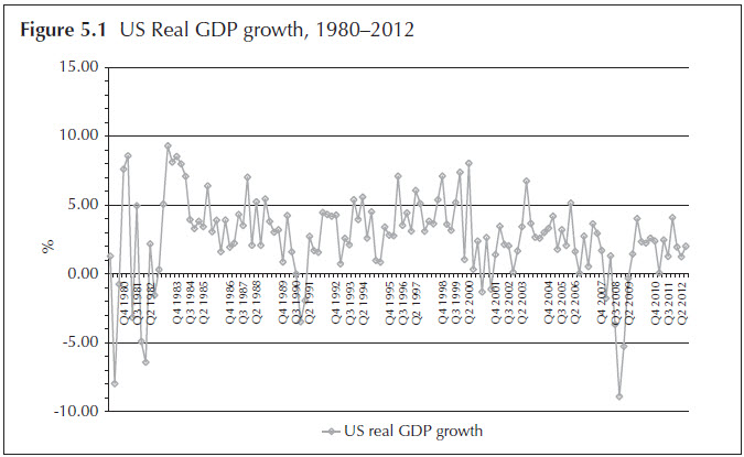
In the U.S., from 1980 to 2013, there have been nine periods of negative economic growth over one fiscal quarter or more (see figure 5.1). According to the National Bureau of Economic Research (NBER), there have been five periods considered recessions:³ 

• January 1980–July 1980: 6 months;
• July 1981–November 1982: 16 months;
• July 1990–March 1991: 8 months;
• March 2001–November 2001: 8 months; and
• December 2007–June 2009: 18 months.

^{Accessible version}

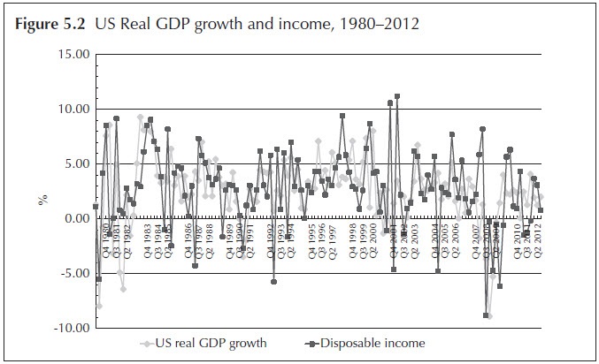
From figure 5.2, we can see that a drop in GDP growth rate is usually associated with a drop in the real disposable personal income growth rate. Thus, we can state, in general, a stress economic condition is associated with a drop in real disposable personal income growth.

^{Accessible version}

From figure 5.3, we can see that the last two recessions are associated with significant drops in the Dow Jones Index, and from figure 5.4 we see that the most severe recession followed a huge drop in the House Price Index. Hence, we can also confidently claim that a stress economic condition is associated with a drop in Dow Jones Index or House Price Index.

^{Accessible version}

^{Accessible version}

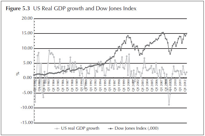
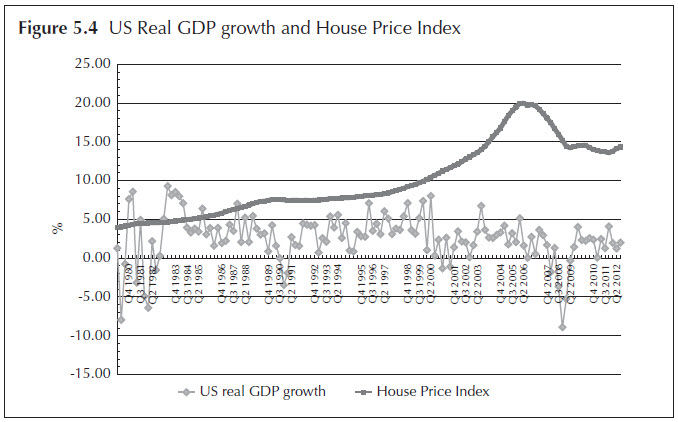
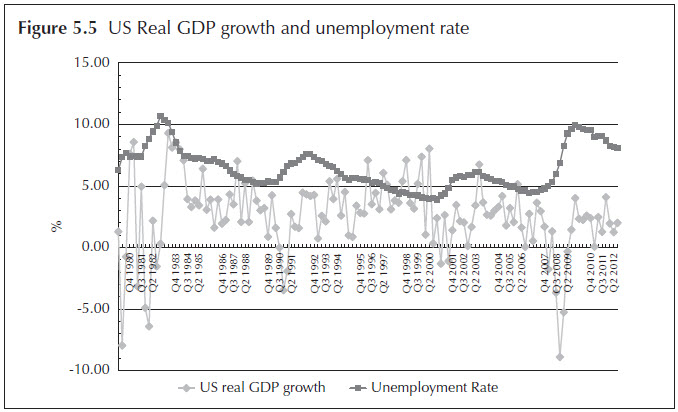
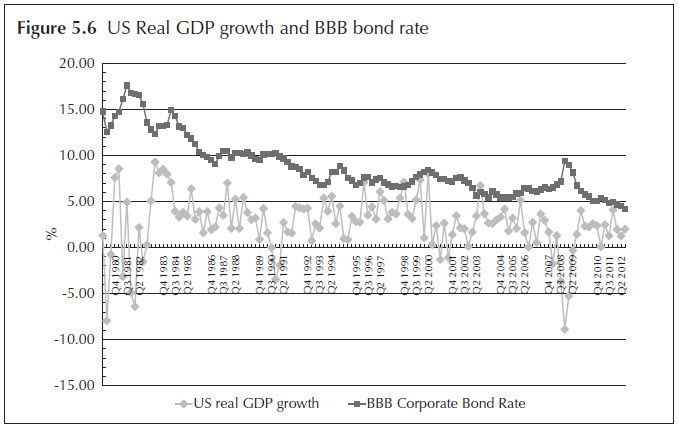
Figure 5.5 clearly shows that each recession was associated with a rise in the unemployment rate. However, for BBB corporate bond rate--although for the recessions in 1981 and 2008 we see a high increase in the BBB rate--the rest of the data does not show a high association between GDP growth rate and BBB bond rate (figure 5.6).

^{Accessible version}

^{Accessible version}

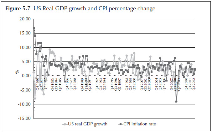
From figure 5.7, we see only that a sharp drop in CPI is associated with the last recession, but, for the rest of the historical data, there is no obvious association between change in CPI and GDP Growth Rate.

^{Accessible version}

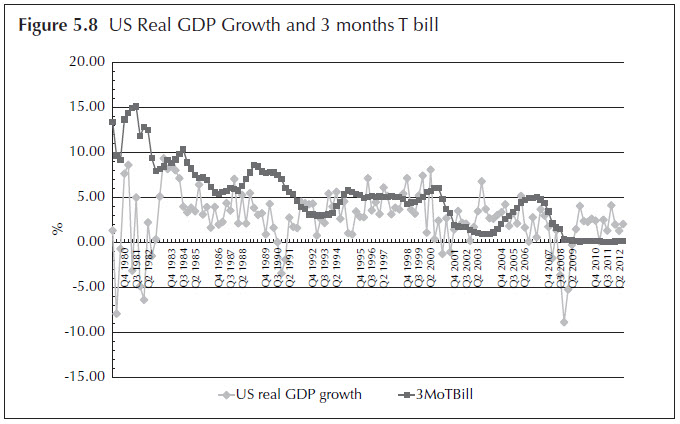
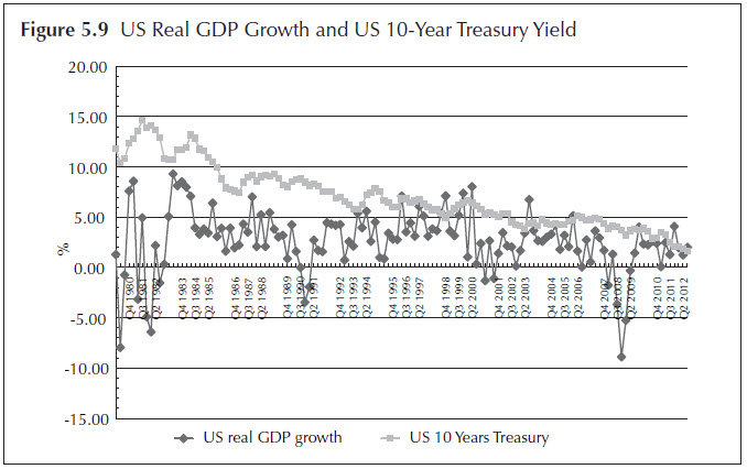
As for the three-month Treasury yield and the U.S. 10-year Treasury yield, from figures 5.8 and 5.9, there is no clear association between real GDP growth rate and Treasury yields. From examining the historical data, of the nine common macroeconomic variables defined in the stress scenarios we have seen that four of them--CPI, three-month Treasury yield, 10-year Treasury yield and BBB corporate bond rate--do not show any "directional" indication that either an increase or decrease in value is necessarily associated with a stress economic condition ("directional" means that, if a macroeconomic variable increases in value, then, historically, the economic condition always reacts the same way, either less or more severe in the same direction). Thus, these four variables will not be further considered in our discussion for measuring the severity of a stress scenario.

^{Accessible version}

^{Accessible version}

Nine-Quarters Projections of the Macroeconomic Variables
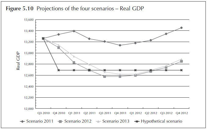
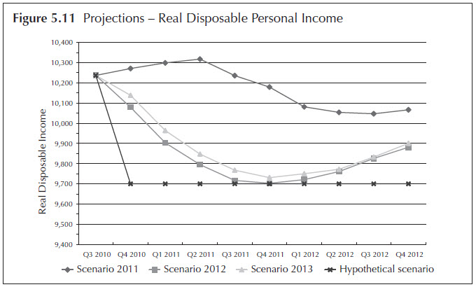
We will now examine the projections of the remaining five macroeconomic variables in each of the four stress scenarios. From figures 5.10 and 5.11, we can clearly see that the 2011 supervisory scenario is the least severe in terms of GDP and real disposable personal income. The 2013 scenario follows the same pattern as the 2012 scenario, but the drop at every quarter is only slightly less than that of 2012. As for the Hypothetical portfolio, it has the biggest drop in disposable income. However, the severity in real GDP is not conclusive because the projected GDP in the Hypothetical are higher than scenarios 2012 and 2013 in some quarters, but lower in other quarters.

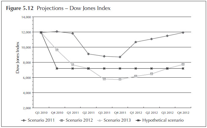
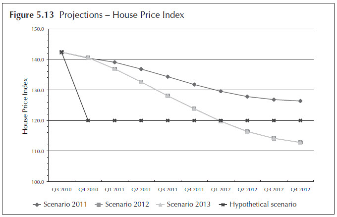
We now focus on the next two "directional" macroeconomic variables: Dow Jones Index and House Price Index. From figures 5.12 and 5.13, we can see that scenarios 2012 and 2013 are exactly the same. The three supervisory scenarios follow similar patterns. On the Dow Jones Index, there is a sharp drop in the beginning, followed by an increase after the fourth quarter, and scenario 2011 shows that the drop is the mildest. As for the House Price Index, the projections are all declining quarter after quarter, and the decline in scenario 2011 is also the mildest. Since the Hypothetical cut across the curve of scenarios 2012 and 2013, by examining the charts, apart from scenario 2011, it is not conclusive which one is the most severe scenario.

Finally, on examining the unemployment rate (figure 5.14), we see that the three supervisory scenarios all project that the unemployment rate will go up over the next six quarters, then plateau, and finally drop slightly at the end. It is also obvious that scenario 2011 is the mildest, and it is inconclusive between the Hypothetical scenario and scenarios 2012 and 2013. By now, we have established that for the three supervisory scenarios--since each of the variables we have seen follows the same pattern, on the whole--scenario 2011 is the mildest, and scenario 2012 and 2013 are almost the same except that scenario 2012 is slightly more severe.

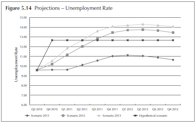
When comparing the Hypothetical scenario with the 2012 and 2013 scenarios in unemployment rate, there are some quarters in which the hypothetical scenario has the higher unemployment rate, and some quarters in which the 2012 and 2013 scenarios have the higher unemployment rate. Therefore, in order to make an overall comparison, it is necessary to develop a statistic to summarize, measure and standardize the severity of each variable over the nine quarters.

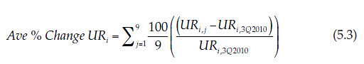
Since we have aligned all the scenarios to the same starting point, the severity of each quarter is determined by the percentage change with respect to the starting quarter (Q3 2010). Thus, a probable summary statistic is the average of the percentage change with respect to the starting quarter. Another choice is the maximum change over the nine quarters, but the maximum value ignores the projections with recovery at the end of the nine quarters. The average of the percentage change is computed by equation 5.3 below, where i is the index for the four scenarios, and j is the index for each of the projections.

This summary statistic can be computed for the five "directional" macroeconomic variables in each scenario. We now have a measure to compare the severity of the scenarios on each of the variables independently of the other variables. From figure 5.15, we can see that the longer the vertical bar is away from zero, the more severity it indicates. Thus, for unemployment rate, the longest bar is in 2013, which means the most severe scenario is 2013. For GDP, disposable income, and HPI, the Hypothetical scenario is the most severe. For Dow Jones Index, the 2012, 2013 and Hypothetical scenarios are more or less the same. Viewing across the chart, we see that the 2011 scenario is the least severe in each of the five variables.

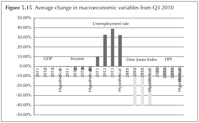
In terms of the magnitude of severity, we see that unemployment rate and Dow Jones Index have 30 percent to 40 percent average deterioration in scenarios 2012, 2013 and the Hypothetical, whereas the other variables are much less severe. Hence, we have a measurement of severity for each macroeconomic variable. In the next section, we will suggest some ways to combine all these measurement to give an overall view of the severity of a stress scenario.

An Overall Assessment of the Severity
At the start of our discussion, we mentioned that measuring severity is, in general, relative. However, some economists (Edge 2012) have tried to use historical recessions as anchors, and relate the stress scenarios to historical recessions to get some sense of magnitude as compared with past recessions. We will discuss other methodologies in more detail in the next section. For now, we will propose a simple methodology to summarize the severity of each scenario with reference to a historical recession.

For each macroeconomic variable, we have four scenarios. We will use an ordinal ranking to assign a rank to each of the scenario by using the Average % Change, giving rankings of 1-4 to indicate least to most severity. When the Average % Change shows that two scenarios are very similar (within 1 percent of each other), we assign the average of the two ranks to both scenarios. Since severity in unemployment rate is associated with increasing value, the lowest rank is given to the lowest Average % Change. Table 5.3 gives the ranking of each variable and the total ranking. By summing across the rank of each variable, we arrive at a statistic that gives an overall ranking (total rank) of the scenarios. With this simple methodology, we have determined the severity of the four macro stress scenarios. In order of severity, the most severe scenario is Hypothetical, followed by 2013, 2012, and 2011. However, on further examination, the differences in total rank between the Hypothetical, 2013 and 2012 scenarios are not that significant (<20 percent), hence these three scenarios are comparable in terms of severity.

Table 5.3 Ranking of each macroeconomic variable and the total rank of the scenario

Scenario	Real GDP		Disposable income		Unemployment rate		Dow Jones		HPI		Total
	Ave % change	RANK	Ave % change	RANK	Ave % change	RANK	Ave % change	RANK	Ave % change	RANK
2011	0.2	1	-0.6	1	9.7	1	-11	1	-6.88	1	5
2012	-4	3	-4.1	2.5	32.4	2.5	-40.8	3	-12.2	2.5	13.5
2013	-3.5	3	-3.7	2.5	38.5	4	-40.8	3	-12.2	2.5	15
Hypothetical	-4.3	3	-5.2	4	32.2	2.5	-39.7	3	-15.7	4	16.5

Since all these four scenarios are hypothetical forward-looking scenarios, and we now have some understanding of the severity among them, the next logical question should be how they are related to our historical experience. Looking back at the past postwar recessions, we see that the most severe recession is the 2008 recession (December 2007 to June 2009), which lasted 18 months. In order to align with the nine projected quarters of our scenarios, we will use the NBER data and choose the consecutive nine quarters of real GDP growth rate when the recession began in the first quarter of 2008. After aligning for Q3 2010 as the starting quarter and the conversion of the values as described in the last section on the remaining nine quarters, we have the similar values on the macroeconomic variables for comparison in table 5.4. The first column has the actual values as in Q3 2010. This is used as the anchor to align all the scenarios that have the same starting values. The rest of the nine columns are from Q1 2008 to Q1 2010 (projections of nine quarters as in all supervisory scenarios). The values in these nine columns are scaled to the starting values of the first column, and so the 2008 recession values start from the second column.

Table 5.4 Nine-quarters values of changes for 2008 recession⁴ 

Common Variables	Q3 2010	Q1 2008	Q2 2008	Q3 2008	Q4 2008	Q1 2009	Q2 2009	Q3 2009	Q4 2009	Q1 2010
Real GDP	13,261	13,202	13,245	13,122	12,820	12,649	12,639	12,684	12,810	12,884
Real disposable personal income	10,237	10,385	10,592	10,350	10,344	10,220	10,208	10,048	10,033	10,172
Unemployment rate	9.58	9.98	10.64	11.98	13.7	16.5	18.49	19.23	19.83	19.49
Dow Jones Index	11,947	10,748	10,540	9,574	7,326	6,541	7,598	8,797	9,269	9,804
House Price Index	142	137	131	126	120	114	112	113	114	115

After we calculate the average percentage change of the five variables over the nine quarters, we find that the average % change on real disposable personal income is slightly positive (0.2 percent). Thus, during the 2008 recession, the real disposable personal income is not "directional," as we once thought. We have come to realize that it is not necessarily true that real disposable personal income will decrease in a severe stress economic condition, especially when we are looking at the overall change in nine quarters. Therefore, including the real disposable personal income will taint our measurement of severity. Hence we will drop the real disposable personal income from our ranking on the overall severity. We can now put the average % change of the rest of the variables back into the ranking methodology and observe the ranking of the recession with other scenarios.

From table 5.5, we observe that 2008 recession is ranked as the most severe, followed by Hypothetical, 2013, 2012, and 2011. However, apart from the unemployment rate in 2008 recession, the differences among the four most stressful scenarios are not so significant that they can be easily separated. In fact, for the Dow Jones Index, 2008 recession is the second least severe of the five scenarios. Hence we conclude that the Hypothetical, 2013 and 2013 scenarios have similar severity to 2008 recession.

Table 5.5 Ranking of each macroeconomic variable and the total rank of the scenario and recession

Scenario	Real GDP		Unemployment Rate		Dow Jones		HPI		Total
	Ave % change	RANK	Ave % change	RANK	Ave % change	RANK	Ave % change	RANK
2011	0.2	1	9.7	1	-11	1	-6.88	1	4
2012	-4	3.5	32.4	2.5	-40.8	4	-12.2	2.5	12.5
2013	-3.5	3.5	38.5	4	-40.8	4	-12.2	2.5	14
Hypothetical	-4.3	3.5	32.2	2.5	-39.7	4	-15.7	4.5	14.5
08 Recession	-2.8	3.5	62.2	5	-25.4	2	-15.5	4.5	15

In all our discussion so far, we have assumed that all the directional variables are of the same importance, hence we have not assigned different weights when aggregating the ranks of each variable. However, we know different macroeconomic variables will affect different banking institutions. For example, banks with large credit-card portfolios are more sensitive to the unemployment rate; banks with large mortgage portfolios are more sensitive to house prices; and banks with large corporate portfolios are more sensitive to real GDP and equity indexes. In addition, the severity of the loss is related to the credit quality of the portfolio. Thus, the severity of the stress scenario also depends on the risk profile and the businesses of a bank. Based on the bank's experience, different weights can be assigned to different variables to emphasize the importance of certain variables.

Other Methodologies of Measuring Severity
Our approach to assessing severity is entirely ordinal and so the relative ranks do not reflect anything about the magnitudes of the average percentage change, or the degree of severities. Ranking the scenarios will necessarily give some scenarios high rankings even if all the scenarios are quite mild, and some scenarios low rankings even if all the scenarios are quite severe. As we saw earlier, our approach is to give relative ranking to the scenarios under consideration. By comparing the scenarios with 2008 recession, we have attempted to give the four scenarios a reference point besides comparing them with each other.

There have been other attempts to quantify the severity of stress scenarios. One of them is to determine the probability of occurrence of a stress (or worst) scenario. The general belief is that the less likelihood there is of an occurrence of a stress scenario, the more severe the stress scenario will be. In the 2009 SCAP exercise, in footnotes 3 and 4 of Federal Reserve (2009b), the supervisors attempted to assign a probability of occurrence to the adverse scenario by claiming that "the likelihood that the average unemployment rate in 2010 could be at least as high as in the alternative more adverse scenario is roughly 10 percent. In addition, the subjective probability assessments … imply a roughly 15 percent chance that real GDP growth could be at least as low, and unemployment at least as high … [and] there is roughly a 10 percent probability that house prices will be 10 percent lower than in the baseline by 2010." Another example appears in an article on Economy.com in which Ed Friedman (2012) assigned probabilities to the Fed's 2013 CCAR scenarios. He first put the probability for each baseline scenario at around 50 percent. Then he claimed, "The Fed's Severely Adverse scenario is comparable to one that Moody's Analytics terms S4. We currently see a 4 percent chance that this scenario will occur. The Fed's Adverse scenario is more puzzling…we believe [it] has about a 10 percent chance of occurring." It seems to us that most of this assigning of probabilities is based on judgement rather than any empirical derivation.

One of the more interesting approaches to quantifying severity is proposed by two Federal Reserve Board economists, Rochelle Edge and Sam Rosen. Their simple approach (2012) is for each scenario, they will score the average % change of the common variables by assigning a value of 100 to the variable if the deterioration in the variable equals what occurred in 2008 recession (most severe), and by assigning a value of 0 to the variable if the deterioration equals what occurred on the average in the two recessions (mild recessions) before 2008 recession. Below, we use a modified version of their approach to illustrate how severity can be quantified.

For each common variable in 2008 recession, we assign a score of 100 for the average % change, and 0 if the average % change is 0. In addition, we cap the score of each variable at 100 and assign a floor of 0. We then use a simple linear interpolation to convert each variable of a scenario into a score. For example, the average % change in UR in 2008 recession is 62.3 percent, and in Scenario 2013 is 38.5 percent. Thus the score for 2008 recession in UR is 100, and for Scenario 2013 is given by the following equation:

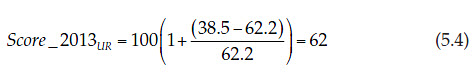
Table 5.6 gives the results of the scoring approach. Using 2008 recession as a reference point, Scenario Hypothetical, 2013 and 2012 are very similar to and a bit less severe than the 2008 recession. The 2011 scenario is the mildest and its average score is quite different from the rest. Although our choices in this approach are sometimes arbitrary, nonetheless the approach is intuitive and informative, and gives a good sense of how the scenarios are compared.

Table 5.6 Score of each macroeconomic variable and the average score of the scenario and recession

Scenario	Real GDP		Unemployment rate		Dow Jones		HPI		Total RANK
	Ave % change	RANK	Ave % change	RANK	Ave % change	RANK	Ave % change	RANK
2011	0.2	0	9.7	16	-11	43	-6.88	44	26
2012	-4	100	32.4	52	-40.8	100	-12.2	78	83
2013	-3.5	100	38.5	62	-40.8	100	-12.2	78	85
Hypothetical	-4.3	100	32.2	52	-39.7	100	-15.7	100	88
08 Recession	-2.8	100	62.2	100	-25.4	100	-15.5	100	100

So far, the approaches we have discussed do not assume any correlations among the four common macroeconomic variables. The overall assessment is made by summing each variable independently. A statistical approach proposed by Debashish Sarkar (2012) attempted to solve the major problems of the aggregating of information across different variables and across time. He suggested using the Mahalanobis distance to solve these problems with a set of weights. The distance, D, is defined by the following equation:

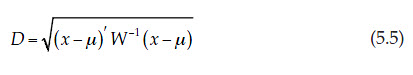
In the formula, X is a vector that stacks different variables in a scenario through time. The vector µ stacks the same variables for a reference scenario. The matrix W collects the weights. This approach is to construct W based on the variance-covariance matrix of the out-of-sample forecast errors. While the main challenge of this approach is that the distance measure is not directional, it is also very sensitive to the choice of W and the reference scenario. Sarkar's results showed that this approach is best used in conjunction with some other methods and is more efficient for identifying outlier/problem scenarios. Similarly, in a somewhat related paper, Breuer et al (2009) also suggested using the Mahalanobis distance to quantify the plausibility of a severe stress scenario.

Lastly, we mention another approach that aggregates the information in different macroeconomic variables through a simple forecasting framework. In their 2012 paper, Guerrieri and Welch (2012) derived several forecasting models to predict some key metrics that measure the "health" of a bank holding company. The key metrics that they wanted to forecast were: net charge-offs on loans and leases, pre-provision net revenue (PPNR), net interest margin (NIM), and the tier 1 regulatory capital ratio. The forecast is based on a set of macroeconomic variables: real GDP growth, unemployment rate, the growth rate of the National House Price Index, the term spread, the growth rate of the S&P 500 Index, the implied volatility of the S&P 500 Index options, and the real interest rate. For each macroeconomic variable Vi and for each key banking metric, C, they used a simple (lag) regression that takes the form:

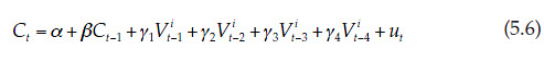
They used the Consolidated Reports of Condition and Income (Call Report) of the Federal Deposit Insurance Corporation to develop their forecasting models. By applying the historical information from the Call Report data and the changes in the macroeconomic variables in the stress scenarios to the forecasting models, we can obtain the forecast estimates of the key metrics. Consequently, we can then use the results, e.g., average forecast charge-offs, to quantify the severity of the scenarios. The usefulness of this approach depends highly on the accuracy of the forecasting models, especially on the later fore- casting quarters. However, Guerrieri and Welch found large root-mean-square errors for the forecasts of all the metrics, and their best-performing model did not beat a random walk at all horizons for forecasting pre-provision net income.

Conclusion
Our approach is based on examining the extremities of each of the directional variables, and adding up the extremities without considering the correlation and the timing of the macroeconomic variables. We have avoided trying to quantify the severity and used ordinal ranking to smooth out the "noises" of the variations. There is no error estimate in our assessment, nor do we give any confidence levels on our assessment: there is a danger of pseudo-accuracy when we try to find precision, and precision is difficult to define. It is exceptionally difficult to validate a model to assess the severity of a stress scenario. In the previous section, we mention that economy.com states that the 2013 Fed Severely Adverse scenario has a 4 percent chance that it will occur. The interesting question is why it is 4 percent and not 10 percent? The figure seems arbitrary. No one will dispute that the 2008 recession is the most stressful economic period since the Great Depression. Using the 2008 recession as a severe stress scenario, someone might say it is a 1-in-80-year event because it is the most severe recession for 80 years. However, if another recession as severe as or more severe than the 2008 recession happens in the next 10 years after 2008, then it reduces the occurrence of such a severe event to a 1-in-45-year event. Thus, it is quite difficult to quantify such a rare event with certainty because any occurrence of a similar event in the future will render the estimate to be inaccurate.

One of the principles of stress testing listed in the 2009 BIS (BIS BCBS 2009) paper is, "Stress tests should feature a range of severities, including events capable of generating the most damage whether through size of loss or through loss of reputation." The challenge is how to define an event that will generate the most damage to a bank. In their paper, Borio, Drehmann and Tsatsaronis (2012) concluded that "stress tests failed spectacularly when they were needed most: none of them helped to detect the vulnerabilities in the financial system ahead of the recent financial crisis." To improve the performance of macro stress tests, they suggested increasing the severity of the scenarios. The financial crisis of 2008 can be used as a starting point to gauge the severity of a bank's stress scenario. According to the above 2009 BIS paper, "prior to the (2008) crisis, however, banks generally applied only moderate scenarios, either in terms of severity or the degree of interaction across portfolios or risk types … Scenarios that were considered extreme or innovative were often regarded as implausible by the board and senior management."

Have the banks learned their lessons? Are they designing severe stress scenarios that will result in estimates of losses that show their vulnerabilities? In this chapter, we have suggested a simple way to answer these questions, and discussed alternate methodologies to answer the same questions. In many countries, banking regulators are requiring banks to perform stress testing on an annual basis. As more data is gathered from these exercises, it will enhance further research on this topic, and hopefully the macro stress tests will become a valuable tool in the banks' risk-management arsenal.

References

BCBS, 2009, "Principles for Sound Stress Testing Practices and Supervision (PDF)," Basel Committee on Banking Supervision.

Borio, Claudio, Mathias Drehmann and Kostas Tsatsaronis, 2012, "Stress-Testing Macro Stress Testing: Does It Live Up to Expectations? (PDF)," January, Monetary and Economic Department, BIS Working Papers No. 369.

Breuer, Thomas, et al, 2009, "How to Find Plausible, Severe, and Useful Stress Scenarios," International Journal of Central Banking 5(3), pp. 205–24.

Edge, Rochelle, and Sam Rosen, 2012, "Assessing the Severity of Macro Scenarios in CCAR," February 3, Federal Reserve System internal document (availability by direct request to authors).

Federal Reserve, 2009a, "The Supervisory Capital Assessment Program: Overview of Results (PDF)," Board of Governors of the Federal Reserve System, May 7.

Federal Reserve, 2009b, "The Supervisory Capital Assessment Program: Design and Implementation (PDF)," Board of Governors of the Federal Reserve System, April 24.

Federal Reserve, 2011a, "Comprehensive Capital Analysis and Review: Objectives and Overview (PDF)," Board of Governors of the Federal Reserve System, March 18.

Federal Reserve, 2011b, "Federal Reserve System, Capital Plan Review, Summary Instructions and Guidance (PDF)," Board of Governors of the Federal Reserve System, November 22.

Federal Reserve, 2012, "2013 Supervisory Scenarios for Annual Stress Tests Required under the Dodd-Frank Act Stress Testing Rules and the Capital Plan Rule (PDF)," Board of Governors of the Federal Reserve System, November 15.

Friedman, Ed, "2012, Bank Stress Scenarios Reflect Fed's Risk Views," November 26, available at: http://www.economy.com/dismal/article_free.asp?cid=235707.

Guerrieri, Luca, and Michelle Welch, 2012, "Can Macro Variables Used in Stress Testing Forecast the Performance of Banks? (PDF)," July 23, Finance and Economics Discussion Series, Federal Reserve Board.

Peristian, Stavros, Donald P. Morgan and Vanessa Savino, 2010, "The Information Value of the Stress Test and Bank Opacity," July, Federal Reserve Bank of New York, Staff Report No. 460.

Sarkar, Debashish, 2012, "Severity Scoring Models for Assessment of BHC Stress Scenarios," February 10, Federal Reserve Bank of New York internal document (availability by direct request to author).

Wyman, Oliver, 2012, "Asset Quality Review and Bottom-up Stress Test Exercise (PDF)," September 28.

---

1. In 2013, six U.S. BHCs were subject to estimate trading losses: Bank of America Corp, Citigroup, Goldman Sachs, JPMorgan Chase, Morgan Stanley, and Wells Fargo & Co. Return to text

2. Historical Data: 1976 through Second Quarter 2012--October 9, 2012 (Excel) – available for download at http://www.federalreserve.gov/bankinforeg/ccar.htm. Return to text

3. See http://www.nber.org/cycles.html. Return to text

4. The nine quarters from Q1 2008 to Q1 2010 are converted to Q3 2010 as the starting values. Return to text