
FEDS Notes
 Print
PrintNovember 21, 2014
November 2014 update of the FRB/US model
Jean-Philippe Laforte and John Roberts
Introduction
This FEDS Note is a companion to the most recent release of the FRB/US model of the U.S. economy on the Board's website. The purpose of this note is twofold. First, it briefly outlines and describes the changes to the structure of the public version of FRB/US since its introduction in the spring of 2014. In addition, it compares the dynamics of the current version to that of the original version in response to key shocks.
Changes to the model
The most recent update of the public version of the FRB/US model differs from its original release in many significant ways.
-
Re-estimation of the stochastic equations: We re-estimated all stochastic equations following the release of the NIPA annual revision in August over a sample period that now extends an additional year to 2013q4.
-
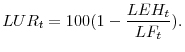
Changes to the specification of the labor market sector: The dynamics of the unemployment rate (LUR) in the original public version of FRB/US were based on an estimated "Okun's law" relationship that directly linked the unemployment rate to the output gap. In the new model, the unemployment rate is related to the levels of civilian employment (LEH) and the labor force (LF) by an identity:
-
Introduction of an estimate of the real gross domestic product adjusted for measurement errors: The updated version of FRB/US introduces an estimate of real GDP that abstracts from measurement error, which we call XGDO. As in the previous version of the model, the published estimate of real GDP, XGDP, is chain-aggregated from various expenditure categories. XGDO is then inferred by adjusting XGDP for an estimate of measurement error (MEP):
XGDO = XGDP/MEP,
The new model also introduces real gross domestic income (XGDI), which is calculated by adjusting XGDO with a second estimate of measurement error (MEI):
XGDI = XGDO × MEI
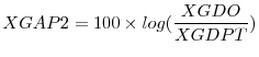
The historical estimates of measurement error are derived from the same model used to estimate the latent supply-side variables of the model; documentation about the supply-side model is available here. For forecasting purposes, measurement error follows a simple time-series process. Finally, we now measure the output gap using XGDO rather than XGDP in the numerator:
-
Switch to overall business-sector output: The focus on productivity in the model was moved from the nonfarm business sector to the overall business sector. The implementation of this change involved the substitution of the series representing nonfarm business concepts (identified by the expression 'XNF;' for example, XNFB) with those of total private business (now identified simply by 'X,' as in XB) and the re-estimation or appropriate recalibration of the equations in which series of the business appear.
-
The re-estimation of the supply-side structure of the model: As with the stochastic equations of the model (see above), the supply-side model that is used to create the latent variables used in FRB/US was re-estimated with a sample that now includes observations from 2013. The structure of the supply-side model was also revised to reflect the switch from nonfarm to total business output. These changes did not have any significant impact on the FRB/US estimates of potential output or the natural rate of unemployment.
-
Changes to the specification of the price-wage sector: In the updated version, the specification of the FRB/US price equation is:
πt = 0.40πt-1 + 0.60πtz + 0.004πt-1 + 0.92μpt-1
where πt is current inflation, πtz is "expected" inflation (ZPICXFE), πt is the long-term inflation expectations (or PTR), and μtp is the price markup gap (see the complete documentation for more details). The key difference between the new and original versions is a reduction of the lag order of the "past inflation" term to one (from four). In addition, the estimation sample now spans the period 1988Q1-2013Q4. The specification of the wage equation has remained the same as in the original version, but its coefficients were re-estimated jointly with those of the new price equation. For both the price and wage equations, the influence of past (price or wage) inflation is now lower than before.
- In addition to the changes to the structure of the model noted above, the following obsolete variables were deleted from the model: FNFIN, FNFIRN, UFNFIR, HPRDTP, HPRDTW, UXGN, UYHPNT, HGVPI.
The impulse responses of the model to key shocks
To illustrate the properties of the FRB/US model, we report the simulated responses of inflation, the output gap, and the federal funds rate to eight key disturbances: shocks to the federal funds rate and term premium; shocks to government spending and to the equity premium; shocks to both the level and growth rate of trend multifactor productivity; and the exchange rate and the price of crude oil. In each case, one-period shocks are applied to specific model equations. The persistence of each shock depends on the properties of the equation in which it appears. Details can be found in the equation documentation in the FRB/US model package.
We show results under the two main expectations mechanisms in the FRB/US model, VAR-based expectations and model-consistent expectations. We assume that monetary policy responds according to an inertial version of the Taylor (1999) rule.2 Computer code with full details on how these simulations were generated is available in the main FRB/US model package.3
The top panels of Figure 1 show the responses of the model to a 100-basis-point shock to the model's inertial Taylor rule. As can be seen, the output responses of the model are little affected by the changes to the model introduced in the November release. The reaction of inflation, however, is less persistent in the new version of the model; this is especially evident for version of the model with the VAR-based expectations. The main reason that inflation is now less persistent is the smaller coefficient on lagged inflation in the new version of the model, as discussed above. As before, the effects of the funds rate shock on output and inflation are considerably smaller in the version of the model with model-consistent expectations. As explained in an earlier note, the differential effects largely reflect differences between the inertial Taylor rule and the estimated funds rate equation that is part of the VAR-based expectations mechanism. The VAR's policy rule has more inertia than the Taylor-type policy rule used for these simulations. As a result, the interest rate increase is anticipated to be more persistent under VAR-based expectations and, because of its effect on real long-term interest rates, which causes the output gap and inflation to decline substantially more in this case.
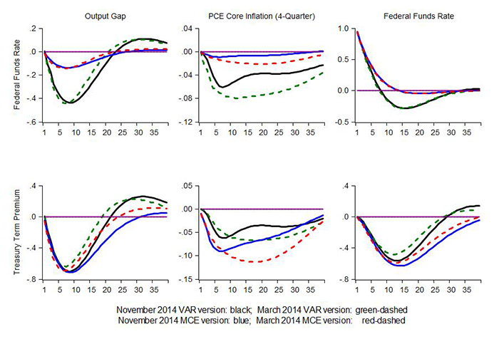
The bottom panels of Figure 1 show the responses of the model to a 100-basis-point shock to the 10-year Treasury term premium.4 As in the previous case, the increases in long-term interest rates depress output and inflation. The federal funds rate declines as the inertial Taylor rule prescribes lower interest rates in response to lower output and inflation. The responses of the economy to the term premium disturbances under MCE and VAR-based expectations are much closer to each other than are the responses to a fed funds rate shock, mostly because the effects of the term-premium shock on longer-term interest rates are very similar in the two versions of the model.
Figure 2 shows the effects of two additional shocks related to aggregate demand. The upper panels shows the responses to a one-quarter shock to the model's equation for federal government spending. The initial shock leads to a persistent increase in government spending owing to the inherent persistence in the model equation for government spending. In both versions of the model, output initially rises by about 1 percent of GDP, in line with the size of the innovation. The higher level of output relative to potential leads to increases in the federal funds rate. These higher interest rates "crowd out" private-sector spending and as a consequence, beyond the initial period, the increase in output is typically smaller than the increase in government spending--that is, the government-spending multiplier is less than one. The effects of the shock differ slightly in the two versions of the model. In particular, after three years, output falls below baseline in the VAR version of the model, whereas it stays close to it in the MCE version.
The bottom panels of Figure 2 display the response to an increase of the equity premium by 100 basis points. The output gap turns negative as higher financing costs faced by firms reduce capital spending and households' spending slows as their equity wealth falls. There is a small decline in inflation that lags somewhat the output gap owing to the model's inflation persistence.
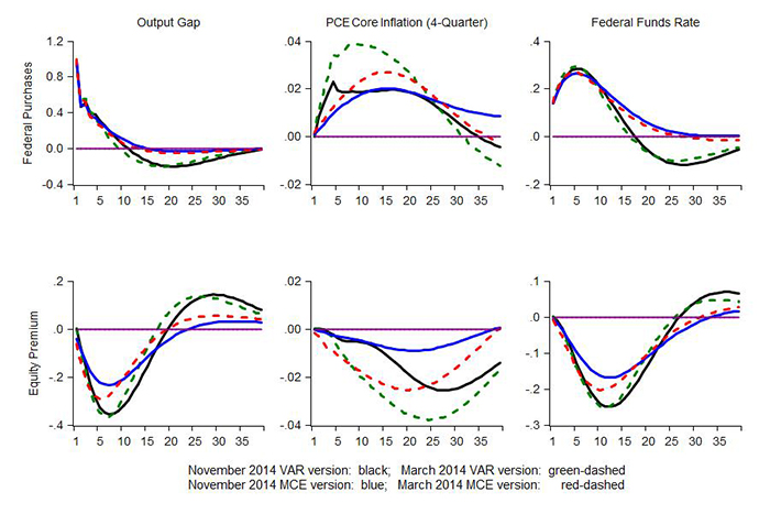
Figure 3 shows the effects of shocks to trend multifactor productivity. The top panels show the effects of an immediate and permanent 1-percent increase in the level of trend MFP. Because spending is inertial in FRB/US, the level of real GDP initially changes very little. As a consequence, the initial jump in the level of potential output implies a drop in the output gap. Inflation also falls, mostly reflecting the reduction in marginal cost associated with the increase in productivity. With both the output gap and inflation depressed, the Taylor rule prescribes a lower federal funds rate. The output gap eventually closes, reflecting both the gradual increase in spending in response to higher permanent income and wealth as well as the stimulative effects of lower interest rates.
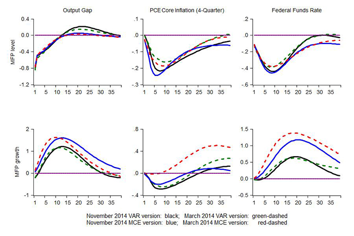
The bottom panels show the effects of an increase in the trend growth rate of MFP that is initially 1 percentage point and then gradually returns to baseline. In this case, spending initially outstrips potential output, as households and firms anticipate higher incomes and wealth before they materialize. Inflation declines, however, reflecting the direct impact of higher productivity on marginal cost. There are thus competing effects on monetary policy. On balance, the positive output gap dominates and the federal funds rate rises.
Figure 4 shows the consequences of changes in two key foreign factors. The top panels display the response of the economy to an initial increase of 10 percent in the exchange rate. An appreciation of the dollar leads to lower exports and higher imports, and thus represents a drag on aggregate demand as seen in the top-left panel. The output gap eventually widens by about 3/4-percentage point after two years in both versions of the model. Thereafter, the output gap returns to baseline more rapidly in the VAR version of the model. Inflation falls below baseline, reflecting both cheaper imports and the negative slack.
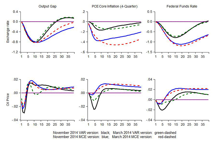
The bottom panels show the effects of a shock to the model's equation for real oil prices that initially raises the price by 10 dollars per barrel. According to the model equation, oil-price movements are not very persistent. The initial effect is a small decline in output, reflecting the depressing effects of higher oil prices on real household incomes and thus on spending. After about a year, however, the output gap turns positive, reflecting both a rebound in spending as well as persistently adverse effects of higher oil prices on the supply-side of the economy in FRB/US. This also explains why core inflation quickly and persistently move above baseline, as shown in the middle panel. Under MCE expectations, inflation barely falls, as the agents already anticipate the gradual and long-lived deterioration in potential.
1. The discrepancy between household and payroll employment also moves cyclically in the new version of the model. Return to text
2. Specifically, let it denote the nominal federal funds rate, r the steady-state real short-term interest rate, πt the four-quarter rate of inflation, πt the inflation objective, and xt the output gap. The policy rule used in the simulations is it = ρiit-1 + (1 - ρi)(r + πt + φπ(πt - πt) + φxxt) + εt, with an interest smoothing parameter ρi of 0.85, and the values for φπ and φx of 0.5 and 1, respectively. Return to text
3. The program pings.prg included in the FRB/US package computes the impulse responses of the eight shocks discussed in this article. Return to text
4. Consistent with the differences in duration, the simulation includes shocks to the 5-year and 30-year Treasury term premiums of 75 and 30 basis points, respectively. Return to text
Please cite as:
Laforte, Jean-Philippe, and John M. Roberts (2014). "November 2014 Update of the FRB/US Model," FEDS Notes. Washington: Board of Governors of the Federal Reserve System, November 21, 2014. https://doi.org/10.17016/2380-7172.0036
Disclaimer: FEDS Notes are articles in which Board economists offer their own views and present analysis on a range of topics in economics and finance. These articles are shorter and less technically oriented than FEDS Working Papers.
