
FEDS Notes
 Print
PrintJuly 31, 2015
Taxonomy of Studies on Interconnectedness
Gazi Kara, Mary Tian, and Margaret Yellen1
For the purpose of this note, "interconnectedness" is defined as a broad set of relationships and interactions among financial market participants. The exact nature of these relationships, however, can vary widely, from a direct contract between two banks to the correlated asset holdings of two mutual funds. The specific institutional setting of these connections may, in turn, affect the type of potential vulnerabilities they create. As institutions form connections, they may contribute to a stronger, more robust system, but they may also create potential channels for the propagation of shocks. Understanding the patterns and stability implications of connections across firms is essential in monitoring the financial system.
This note provides a taxonomy of existing studies in the literature on interconnectedness, focusing specifically on empirical measures. Our taxonomy draws together the diverse interconnectedness literature to provide a framework for holistically thinking about and evaluating financial interconnectedness. We begin by discussing an overview of the structure of the taxonomy, which broadly separates measures into network and non-network approaches. Next, we delve into various network and non-network measures, with an emphasis on the pros and cons of each kind of analysis. To provide context for these measures moving forward, we conclude with a discussion of the implications of interconnectedness for financial stability.
Overview of Taxonomy
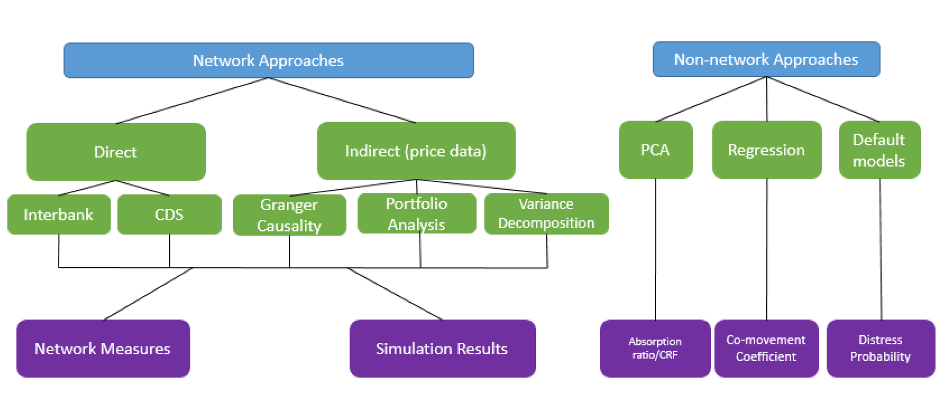
We separate the literature into two broad categories: network approaches and non-network approaches. The network approaches explicitly map the pairwise relationships of individual institutions, which are then used to calculate various analytical measures of interconnectedness and/or to run simulations to obtain measures of fragility of the system. Non-network approaches, meanwhile, use econometric techniques to calculate measures of interconnectedness either for the system as a whole or for pairs of institutions. What differentiates the two approaches is that network approaches take the mapping of pairwise relationships of institutions (e.g. the network graph) as an input in computing measures of interconnectedness, while non-network approaches do not utilize a network graph to measure interconnectedness.
As the figure above demonstrates, our taxonomy portrays three color-coded levels of distinctions between studies: the type of approach (in blue), the type of analysis (in green), and output measures (in purple).
The next two sections explain the different kinds of analysis and output measures within the network and non-network approaches.
Category A: Network Approach
Network analysis draws from the mathematical field of graph theory to model and measure connected systems. A network, or "graph," is simply a collection of points, or "nodes," connected together by lines, or "edges." In directed graphs, the edges point from one node to another to demonstrate a certain flow of information, money, or even disease. In a weighted graph, the edges carry weights to indicate the strength of a given connection. The underlying interpretation of nodes and edges depends on the application. In economics, the nodes are frequently banks or firms; the edges can be anything from interbank lending connections to portfolio similarities.
The framework across financial network studies is fairly standard: Researchers construct a pairwise directed network matrix, using a visual representation (a "graph") to depict those connections. For example, Figure 1 shows a connection matrix for three economic entities--such as banks. Entry x13 in the matrix gives us the strength of the link from Bank 1 to Bank 3; entry x31 tells us the strength of the link in the opposite direction, from Bank 3 to Bank 1. Figure 2 shows the graphical representation of this matrix.

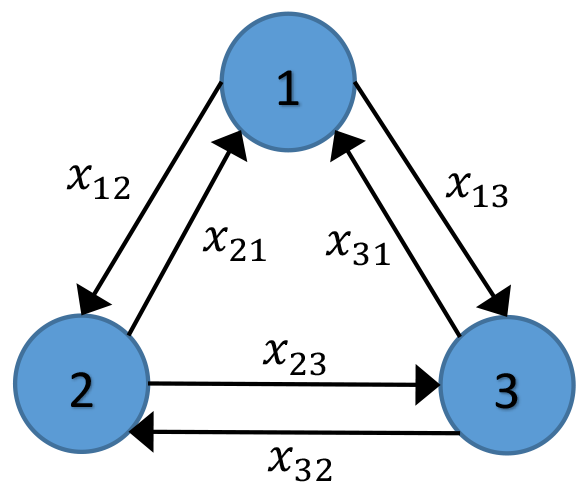
The key difference across studies in the network approach category is what the connections in the graph purport to measure. Here, we distinguish between two branches of studies within the network approach: direct and indirect networks. Direct networks build connections using contractual obligations between banks, such as those stemming from inter-bank lending and borrowing. In a typical direct network, x13 tells us the amount Bank 1 owes Bank 3; x31 is the amount Bank 3 owes Bank 1. In these networks, the diagonal entries are typically set to 0, as banks have no direct contractual obligations to themselves.
In indirect network analysis, pairwise economic connections are inferred from market price data--such as equity returns and portfolio holdings--using a range of empirical techniques. Here, x13 is an estimated connection from Bank 1 to Bank 3. This connection may pick up on the interbank lending relationships between banks, but it may also pick up less obvious sources of connection, such as exposures to common market forces.
Building the Network
The first step in any network approach is building the connection matrix itself; this section explains the process for direct and indirect networks.
Direct networks use raw data on contractual obligations; the two most common types are interbank lending networks and credit swap networks. With complete interbank exposure data, these matrices are simple to construct. Studies from the Swiss, Hungarian, and Czech central banks,2 for example, use regulatory data to construct complete directed interbank lending networks.
With incomplete interbank exposure data, however, researchers must estimate the relationships between banks in the sample. Using data on the total assets and liabilities of each bank, they use entropy maximization3 to fill in the missing individual matrix entries. Authors also sometimes estimate direct network matrices using other kind of obligations, such as credit default swaps. Markose et al. (2012), for example, conduct an empirical reconstruction of U.S. CDS networks based on FDIC call reports data. They define entry xij as the amount of CDS protection bank i is providing to bank j; this is estimated by taking bank j's market share of the CDS buy side multiplied by bank i's gross negative fair value.
Indirect networks, meanwhile, rely on econometric estimation to generate the entries in the matrix. Using data such as equity returns and portfolio holdings, studies can be classified by one of the following three analytical techniques used to estimate empirical connections:
Granger Causality Tests: These tests establish links between institutions using regressions of historical equity returns data. In the network graph, an arrow is drawn from bank j to bank i if bank j Granger-causes bank i, that is, if bank j's returns can forecast bank i's future returns after controlling for bank i's current returns. Billio et al (2012) use Granger-causality tests to build a network using monthly equity returns of banks, broker/dealers, insurance companies, and hedge funds, and then compute network-based measures of connectedness such as degree of Granger-causality, number of connections, and eigenvector centrality.
Variance Decomposition: Developed in Diebold and Yilmaz (2014), this approach uses equity return volatility data, where entry xij in the matrix is the percent of forecast error variance of firm i due to shocks from firm j (estimated using VAR). Once the network is constructed, measures of network centrality, such as total directional connectedness, are computed.
Common Portfolio Holdings: Institutions can be connected through common portfolio asset holdings--here, edge weights measure the commonality of assets held. A price impact function, that is, how much a portfolio's price moves as a result of the other fund selling a certain amount, is used as a proxy for the commonality of assets held. Braverman and Minca (2014) apply this approach to mutual funds' portfolio holdings and construct a "vulnerability index", equal to the sum of a fund's exposures through common asset holdings to other funds.
Using the Network:
Once the network graph is built, studies draw from the insights of graph theory to quantitatively describe the structure of the network. Common network measures in this area include:
- In an interbank network, betweenness shows to what degree a given bank channels funds between other banks in the network.
- Alves et al (2013) note that proximity measures such as closeness centrality can capture the relative importance of banks as suppliers of funding in the interbank market.
- In an indirect Granger causality network, the number of outgoing connections of a bank shows how widespread of an effect that bank's equity price changes have on the network as a whole.
Appendix A provides a list of additional measures, along with their mathematical definitions.
Direct networks, in particular, also form useful foundations for simulations. After setting up the matrix of connections, researchers apply a shock to a randomly selected bank in the sample, causing it to default. Then, they use the interbank matrix to understand how the default of this initial bank affects the balance sheets of connected banks. The process continues through several periods, providing a model of contagion. Although we could ostensibly use indirect networks for simulations, the causal chains in those networks--where edges do not correspond to direct contractual relationships--are not as easy to understand.
By running simulations, researchers can calculate measures of fragility based on the interconnectedness captured in the network. Such measures include number of induced failures, capital lost (in percent of total capital), absolute hazard (number of simulations in which that particular bank fails), and hazard ratios (percentage of failures relative to the number of simulations conducted). They can also calculate contagion rounds (how many rounds it takes the algorithm to converge to the case where no further failures occur).
Of note, conducting simulations relies heavily on assumptions about loss-given-default parameters or how financial institutions respond over time to the initial failure(s), any anticipated cascades, and the underlying conditions/shocks that created them. For example, they assume that banks do not adjust their balance sheets between periods--the contagion, in effect, occurs instantaneously.
Pros and Cons of the Network Approach
Direct networks have many appealing features. They can be constructed using only one cross-section of data, and they are easy to interpret since they use direct bank exposure data. Finally, simulations can be conducted on the networks, giving insight into possible paths of contagion.
On the other hand, direct networks may be difficult to use in time-sensitive policy work. Often, they require supervisory data to build--and, if they use balance sheet data, they can only be updated quarterly with a long lag. In addition, simulations require making a wide range of assumptions--including the common, unrealistic assumption that shocks to the system do not change the underlying network relationships.4 Several papers have also shown that results can change significantly depending on parameter assumptions.
One advantage of indirect networks is that they use market price data, which is readily available at a high frequency and may reflect new information more rapidly than the direct exposure or balance sheet data used in the direct network papers. Because of this, a time-series measure of interconnectedness could quickly be assembled using measures derived from indirect networks. In particular, computing the percentile of the latest period's interconnectedness measure relative to the past history may be informative about current levels of interconnectedness.
On the other hand, indirect networks do not provide as direct of a measure of interconnectedness as the balance sheet and exposure data. Thus, economic interpretations of the measures are not as clear as those estimated from direct networks. Rather than using direct data on obligations, these networks must use estimates of interbank connections--estimates which generally require a time-series of data, rather than a cross-section, to compute. These estimations also make the network reliant on underlying assumptions. The choice of regression specifications in a Granger causality network, for example, will affect the connection entries in the network matrix. Data filtering choices, too, can make a significant difference in the estimated measures of interconnectedness.
Category B: Non-network Approach
Non-network approaches encompass an extremely diverse group of measures. We have placed them into three main sub-categories:
Principal Components Analysis (PCA): PCA takes the underlying equity returns of a set of financial institutions and determines a set of underlying orthogonal factors, called the principal components. Once we have the PC, we can compute the percentage of variation determined by the first n PC. A higher percentage indicates more unified sources of risk--and more interconnectedness in the system.
Co-Movement Factor Regressions: These regressions try to measure connectedness through co-movement of equity returns with common factors. For example, CAPM looks at how much a firm's returns co-move with the market portfolio; the coefficient, the market beta, can be interpreted as a measure of interconnectedness. Unlike networks of common portfolio holdings, which examine the similarities in asset holdings between two individual institutions, these regressions look at co-movement of equity returns with a common market factor.
Default Probability Models: A variety of default probability models try to understand the potential for distress in the system--which is related to the systemic risk/contagion literature.
- Co-risk measures the relationship between the CDS spreads of different banks during times of distress, using regressions that control for common aggregate risk factors.
- Distress dependence takes a broader view by measuring the probability of distress of one bank, conditional on the distress of another.
- Some studies model default intensity as a continuous-time stochastic process with jumps to produce an estimate for the probability of widespread bank failure.
Pros and Cons of Non-network Approaches
Principal components analysis is an appealing technique that provides an easy to compute measure of interconnectedness that can be tracked over time. Although the approach uses underlying equity returns, the PCA vectors themselves need not correspond to economic phenomena and may be challenging to interpret economically.
Co-movement regressions are also relatively simple to implement and estimated betas have an intuitive appeal. However, betas may be slow to update when there are shocks to the financial system, as it may take many periods of extreme returns to significantly alter the economic magnitudes of the betas.
Default probability models are informative as they quantify the probability of distress in the financial system. However, these models may be difficult to estimate and require making additional assumptions, such as parameters of stochastic process for defaults. These different assumptions, in turn, will likely lead to different results.
Implications of Interconnectedness for Financial Stability
The academic literature does not provide definitive answers on whether interconnectedness is good or bad for financial stability. A seminal paper by Allen and Gale (2000) argued that interconnectedness is associated with improved financial stability. In an interbank liquidity risk model, this paper showed that more complete networks provide better risk diversification opportunities, and hence they are less susceptible to contagion compared to incomplete networks. However, recent economic research and the events of the financial crisis have challenged this argument by showing that interconnectedness does not always lead to greater financial stability.
Current discussions on interconnectedness focus on the trade-off between more benefits from direct links versus greater exposure to the risk of default through increased number of linkages. This tension generates networks that are known as "robust-yet-fragile": that is, the very features that make the system stronger under certain conditions may be sources of instability under another. Acemoglu et al. (2013) show that when the magnitude of negative financial shocks are small, more complete networks are less prone to systemic failures because the losses are absorbed by a large number of counterparties. However, when shocks are larger than a threshold, incomplete networks emerge as more stable than complete networks: in a sparsely connected network, losses of a distressed bank are borne mainly by its creditors and are less likely to spread to the rest of the network.
Some recent research also draws attention to the greater complexity and opaqueness brought by more interconnected networks. Caballero and Simsek (2013) argue that complexity of interconnected networks is a dormant factor in normal times; however, when adverse shocks hit, a combination of complexity and uncertainty becomes a source of instability. They show that if banks lack information on their indirect exposures to liquidity shocks through counterparties of their counterparties, instead of buying the assets of the distressed institutions, they start hoarding liquidity or turn into sellers themselves. This results in a fire sale of banks' assets where assets are traded below their fundamental value, which in turn worsens the initial liquidity problem in the system. Gai et al. (2010) also show that greater complexity and concentration in financial linkages can generate systemic liquidity crises. They show that the instability of a financial network depends on the level of liquid asset holdings, the amount of interbank activity, and the size of haircuts on collateral in repo transactions. Allen, Babus and Carletti (2010) show that when the financial system is mainly funded by short-term debt, creditors are less likely to roll-over debt in more clustered networks. There reason is that defaults are more concentrated in clustered networks than in the un-clustered network.
In sum, recent research suggests that whether interconnectedness improves or weakens financial stability depends on many factors, including the magnitude and type of financial shocks, maturity structure of banks' liabilities, existence of information problems and other financial frictions. Studies referenced above have shown that more interconnected networks are more prone to systemic instability under large negative financial shocks, especially when these shocks are combined with short-term funding, imperfect information, and other financial frictions.
Conclusion
The literature on interconnectedness offers a diverse range of potential measures. In weighing the trade-offs between various types of interconnectedness measures, several factors may be particularly useful to consider: the economic content of network versus non-network measures; how quickly measures reflect shocks to the financial system; and the frequency with which the data necessary to build the network can be obtained.
References
Direct Networks:
Allen, Franklin, and Ana Babus. "Networks in Finance." In Network-based Strategies and Competencies, edited by Paul Kleindorfer and Jerry Wind, Wharton School Publishing (2010).
Allen, Franklin, and Douglas Gale. "Financial Contagion." Journal of Political Economy, 108, no.1 (2000):1-33.
Alves, I., S. Ferrari et al. "The Structure and Resilience of the European Interbank Market." Occasional Paper Series, European Systemic Risk Board (2013).
Arciero, Luca, Heijmans, Heuver, et al. "How to Measure the Unsecured Money Market? The Eurosystem's Implementation and Validation using TARGET2 data." De Nederlandsche Bank Working Paper 369.
Battison, Stefano, Michelangelo Puliga, Rahul Kaushik, Paolo Tasca, and Guido Caldarelli. "DebtRank: Too Central to Fail? Financial Networks, the FED and Systemic Risk." Science: Scientific Reports (2012).
Bluhm, Marcel and Jan Pieter Krahnen. "Systemic Risk in an Interconnected Banking System with Endogenous Asset Markets: [version 30 march 2014]." (2014).
Boss, M., H. Elsinger, M. Summer and S. Thurner (2004). "Network topology of the interbank market." Quantitative Finance 4, no.6 (2004): 677-684.
Caballero, Ricardo J., and Alp Simsek. "Fire sales in a model of complexity." The Journal of Finance 68, no. 6 (2013): 2549-2587.
Caccioli, Fabio et al. "Stability of financial contagion due to overlapping portfolios." October22, 2012.
Daron Acemoglu, Asuman Ozdaglar, and Alireza Tahbaz-Salehi. "System Risk and Financial Stability in Networks." American Economic Review, forthcoming.
Degryse, Hans, and Gregory Nguyen. "Interbank exposures: an empirical examination of systemic risk in the Belgian banking system" National Bank of Belgium Working paper (2004).
Drehmann, Mathias and Nikola Tarashev. "Measuring the systemic importance of interconnected banks." BIS working paper no. 342, March 2011.
Elliott, Matthew et al. "Financial Networks and Contagion." American Economic Review (2014). 104(10): 3115-3153.
Gai, Prasanna, Andrew Haldane, and Sujit Kapadia. "Complexity, concentration and contagion." Journal of Monetary Economics 58, no.5 (2011): 453-470.
Hausenblas, Vaclav, Ivana Kubicova, Jitka Lesanovska, (2012). "Contagion Risk in the Czech Financial System: A Network Analysis and Simulation Approach". Working Paper, Czech National Bank.
Iori, Giulia, Roasrio N. Mantegna, Luca Marotta, Salvatore Micciche, James Porter, and Michele Tumminello. "Networked relationships in the e-MID Interbank market: A trading model with memory." Journal of Economic Dynamics and Control, 2014
Jo, Jae Hyun. "Managing systemic risk from the perspective of the financial network under macroeconomic distress." BIS (2012).
Larry Blume, David Easley, Jon Kleinberg, Robert Kleinberg and Eva Tardos. "Network Formation in the Presence of Contagious Risk." Proceedings of the 12th ACM Conference on Electronic Commerce, 2011.
Lelyveld, Iman and Franka Liedorp. "Interbank Contagion in the Dutch Banking Sector: A Sensitivity Analysis." International Journal of Central Banking, 2006.
Lubloy, Agnes "Topology of the large-value Hungarian transfer system." No. 57. Magyar Nemzeti Bank, Occasional Papers, 2006.
Muller, Jeannette. "Interbank Credit Lines as a Channel of Contagion." Journal of Financial Services Research 29, no. 1 (2006): 37-60.
Nitschka, Thomas. "Banking sectors' international interconnectedness: Implications for consumption risk sharing in Europe." Swiss national bank working paper, 2012.
Sheldon, George and Martin Maurer. "Interbank Lending and Systemic Risk: An Empirical Analysis for Switzerland." Swiss Journal of Economics and Statistics 134 (1998): 685-704.
Upper, Christian. "Contagion Due to Interbank Credit Exposures: What Do We Know, Why Do We Know It, and What Should We Know?" Bank for International Settlements, working paper (2006).
Wells, Simon. "Financial interlinkages in the United Kingdom's interbank market and the risk of contagion." Bank of England, working paper. (2002).
Indirect Networks:
Billio, Monica, Mila Getmansky, Andrew Lo and Lora Pelizzon. "Econometric measures of connectedness and systemic risk in the finance and insurance sectors." Journal of Financial Economics, 104, (2011): 535-559.
Bisias, Dimitrios, Mark Flood, Andrew Lo, and Stavros Valavanis. "A Survey of Systemic Risk Analytics." US Department of Treasury, Office of Financial Research, Working Paper (2012).
Braverman, Anton and Andreea Minca. "Networks of Common Asset Holdings: Aggregation and Measures of Vulnerability." Mimeo (2014).
Diebold, Francis and Yilmaz, Kamil. "On the Network Topology of Variance Decompositions: Measuring the Connectedness of Financial Firms." Journal of Econometrics, 182 (2014): 119-134.
Markose, Sheri, Simone Giansante and Ali Rais Shaghaghi. Too interconnected to fail' financial network of US CDS market: Topological fragility and systemic risk." Journal of Economic Behavior and Organization, 83, no. 3 (2012): 627-646.
Non-Network Measures:
Basurto, Miguel and Charles Goodhart. "Banking Stability Measures." IMF Working Paper No. 09/4
Billio, Monica, Mila Getmansky, Andrew Lo and Lora Pelizzon. "Econometric measures of connectedness and systemic risk in the finance and insurance sectors." Journal of Financial Economics, 104 (2011): 535-559.
Chan-Lau, Espinosa, Marco Espinosa, Kay Giesecke, and Juan A. Sole. "Assessing the Systemic Implications of Financial Linkages." IMF Global Financial Stability Report, 2 (2009).
Drehmann, Mathias and Nikola Tarashev. "Measuring the systemic importance of interconnected banks." BIS working paper no. 342 (2011).
Giesecke, Kay, and Baeho Kim. "Risk Analysis of Collateralized Debt Obligations." Working Paper (Palo Alto, California: Stanford University) (2009).
Kritzman, Mark, Yuanzhen Li, Sebastien Page, and Robert Rigobon. "Principal Components as a Measure of Systemic Risk." Journal of Portfolio Management, 37, no. 4, (2011): 112-126.
Podlich, N. and Michael Wedow. "Are insurers SIFIs? A MGARCH model to measure interconnectedness." Applied Economics letters, 20, no.7 (2012).
Appendix A: Network Centrality Measures
 |
|---|
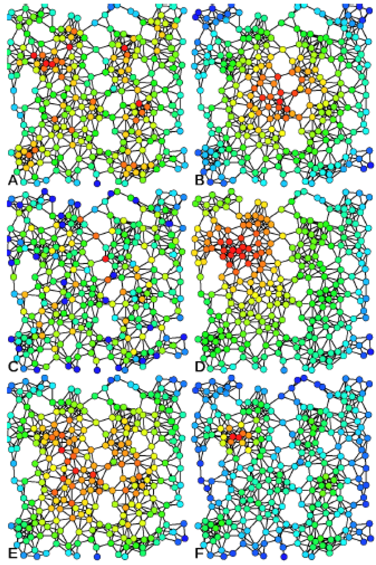
Examples of A) Degree centrality, B) Closeness centrality, C) Betweenness centrality, D) Eigenvector centrality, E) Katz centrality, and F) Alpha centrality on the same graph.
Source: https://en.wikipedia.org/wiki/File:Centrality.svg
As the image above shows, the same graph can have different focal points, depending on the mathematical measure we focus on. The image5 shows exactly the same network, color-coded to show the intensity of six different measures (red is highest value): degree centrality, closeness centrality, betweenness centrality, eigenvector centrality, Katz centrality, and Alpha centrality. This section provides a brief sampling of such graph theoretical measures, which could potentially be applied to financial networks.
Average in-degree/outdegree: The degree of a node is the number of edges connected to that node; in a directed graph, "in-degree" counts edges pointing to the node, "out-degree" edges pointing away. Simply the average of the degrees of all nodes in the graph.
Average shortest path length: SPL is the minimum number of nodes it takes to get from any node A to another node B. Then average the SPL between all pairs of nodes in the graph.
Betweenness Centrality:
![]()
![]() is the number of shortest paths between s and t, and
is the number of shortest paths between s and t, and
![]() is the number of those shortest paths that go through v.
is the number of those shortest paths that go through v.
Centralization: A measure of how central the most central node is, compared to all other nodes (can be used with any underlying measure of centralization)
Closeness Centrality: The inverse of the sum of shortest distances to all other nodes in the graph. Thus, the closer the node to all other nodes, the higher its centrality.
Dissimilarity Index: Provides a measure of how similar/dissimilar two nodes are, based on their distances from other nodes in the graph. Zhao (2003) plugs the dissimilarity indices into an algorithm to identify clusters in the network-groups of similar nodes.
Eigenvector Centrality: Weights a node's centrality by the centrality of connected nodes:
![]()
![]() is the adjacency matrix, so
is the adjacency matrix, so ![]() = 1 if v is linked to t, and 0
otherwise. A particular variant of this measure is PageRank centrality, the google search algorithm that identifies important nodes (for them, websites) by the number and importance of links they connect to.
= 1 if v is linked to t, and 0
otherwise. A particular variant of this measure is PageRank centrality, the google search algorithm that identifies important nodes (for them, websites) by the number and importance of links they connect to.
Percolation centrality: Differs from other measures because value of the node takes into account the "state" of the node. As contagion spreads over the links of a network, it alters the state of the node as it spreads (e.g. states can be binary (infected/no infected), discrete (susceptible/infected/recovered), continuous); percolation centrality measures importance of nodes in aiding contagion through the network
Transitivity coefficient: Shows how likely it is that banks linked to bank A are also linked to other banks linked to bank A
Reciprocity: Measure of mutual exposures-number of exposures that have a corresponding counter-exposure
Appendix B: Entropy Maximization
Because of limited academic access to complete bank balance sheet data, many direct network papers focus on generating an interbank exposures matrix given limited data. Three approaches stand out, and this appendix provides technical details for those interested.
Entropy maximization: Often, researches can only access aggregate asset and liabilities-that is, the row and column aggregates in the interbank matrix. In order to fill the individual entries, they then maximize the entropy of the matrix, which amounts to spreading the loans equally across other banks. Although this method is convenient in the absence of granular data, the assumption of equal lending relationships is not realistic.
Wells (2004) provides an overview of the mathematical process in an appendix. In order to simplify the problem of maximizing the entropy, researchers often normalize the stock of interbank assets and liabilities to unity
![]() . Borrowing from that paper, the mathematical expression of the problem is:
. Borrowing from that paper, the mathematical expression of the problem is:
Subject to:


![]()
We can then obtain the solution:
![]()
The solution above shows that the entropy maximization technique results in a proportionate distribution of bank i's interbank assets (![]() ) to all other banks in the network, weighted by
their interbank liabilities (
) to all other banks in the network, weighted by
their interbank liabilities (![]() ). This model above assumes that banks to have exposures to themselves; in order to create a more realistic image, we can create a new matrix by setting the
diagonal values in the matrix to zero. Then, we need to minimize the cross-entropy between the altered matrix and the original matrix.
). This model above assumes that banks to have exposures to themselves; in order to create a more realistic image, we can create a new matrix by setting the
diagonal values in the matrix to zero. Then, we need to minimize the cross-entropy between the altered matrix and the original matrix.
Entropy maximization with large exposures data: The basic technique for completion remains the same; however, information on large exposures constrains the matrix. Researchers fill the entries for which they have information, then maximize the entropy of the rest.
Furfine federal funds method: Furfine (1999) uses the federal funds wire to match banks and identify loans. Dan Li (FRS) uses a similar method; for more details, see those two papers.
1. Board of Governors of the Federal Reserve System. Email: [email protected]; [email protected]; [email protected]. The analysis and the conclusions set forth are those of the authors and do not indicate concurrence by other members of the research staff or the Board of Governors of the Federal Reserve. Return to text
2. Muller (2006); Lubloy (2006); Hausenblas et al. (2012). Return to text
3. See Appendix B for mathematical definition. Return to text
4. For example, Wells (2002) show simulation results can change depending on assumptions about loss given default parameters. Return to text
5. https://en.wikipedia.org/wiki/File:Centrality.svg Return to text
6. For details, see Wells (2004). Return to text
Please cite as:
Kara, Gazi Ishak, Mary Tian, and Margaret Yellen (2015). "Taxonomy of Studies on Interconnectedness," FEDS Notes. Washington: Board of Governors of the Federal Reserve System, July 31, 2015. https://doi.org/10.17016/2380-7172.1569
Disclaimer: FEDS Notes are articles in which Board economists offer their own views and present analysis on a range of topics in economics and finance. These articles are shorter and less technically oriented than FEDS Working Papers.
