After having been a relatively bright spot early in the recovery, nonresidential private fixed investment, which in this note we refer to as business fixed investment (BFI), increased at an average annual rate of only about 4 percent in 2012 and 2013, an unusually slow pace during an expansion. Given the importance of investment both for understanding cyclical variation in the economy and for potential output growth, we explore this weakness from two alternative perspectives and conclude that it is not particularly surprising.

As was typical in previous business cycles, changes in BFI were an important component of the cyclical swings during the most recent recession and recovery. As shown in the left panel of Figure 1, BFI declined a cumulative 20 percent during 2008 and 2009 and then rose 17 percent over the subsequent two years. These movements were large by historical standards, as would be expected given the depth of the recent recession.

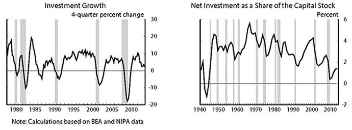
The large decrease in investment in 2009 brought down the level of BFI so substantially that investment was barely sufficient to keep up with the replacement of depreciated capital. As shown in the right panel of Figure 1, net investment as a share of the capital stock (which is equivalent to the growth rate of the real capital stock) fell to its lowest level since World War II. Although net investment has rebounded some in the ensuing years, it remains quite subdued, hovering around 1½ percent per year.² The stepdown in the level of net investment since the recession also has led to a decline in the contribution of capital deepening (capital services per trend employee hour) to the growth rate of trend labor productivity and thus to potential output growth.

Perspective 1: A standard "accelerator"-style model

One way to assess whether recent investment growth is unusually low is to compare it to the predictions of a standard model. A basic neoclassical investment model, in which a representative firm chooses capital spending to maximize expected future profits (assuming a Cobb-Douglas production function for ease of exposition), yields the result that the optimal choice for the log of the capital stock in the absence of frictions will be:

where is a constant, is the log of business output, and is the log of the user cost of capital.³ Note that taking the difference of this equation twice yields the familiar result that the change in net investment is related to the acceleration in output--a relationship that gives its name to the "accelerator" mechanism described in Samuelson (1939).

In our implementation, which follows an aggregate version of Tevlin and Whelan (2003), we use a more general form of the production function, and we allow for additional elements like capital depreciation and adjustment costs (which we assume are quadratic). We also assume that firms form expectations of future output and the user cost rationally, and we use methods proposed by Hansen and Sargent (1980) to solve for . Taking differences yields the basic estimating equation.

To illustrate the predictions from this model, we focus on equipment and intellectual property products (E&I) as these categories of BFI are much larger, move more contemporaneously with GDP, and play a more important role in capital deepening than the remaining category (nonresidential structures). The left panel of Figure 2 shows the latest data along with an out-of-sample prediction for growth in real E&I investment from the accelerator model. The model estimation uses data through the end of 2007, while the model simulation incorporates data on the right-hand side variables (business output and the user cost) through the end of 2013. Investment growth was considerably above the model in 2010-11, but fell short of the model's prediction in 2012 (an error of about 3 percentage points). In 2013, the model appears to explain E&I growth fairly well.

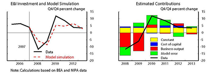
The right panel of Figure 2 shows a decomposition of E&I growth into its various model determinants. The yellow portions of the bars roughly represent the constant term in the model. Usually, investment growth, the black line, would be far above this constant level during a recovery because of robust business output growth. However, in 2012 and 2013, the contribution to investment growth from business output (the red portions of the bars) was only marginally positive, on net, an important reason for the sluggish pace of investment over the past two years.

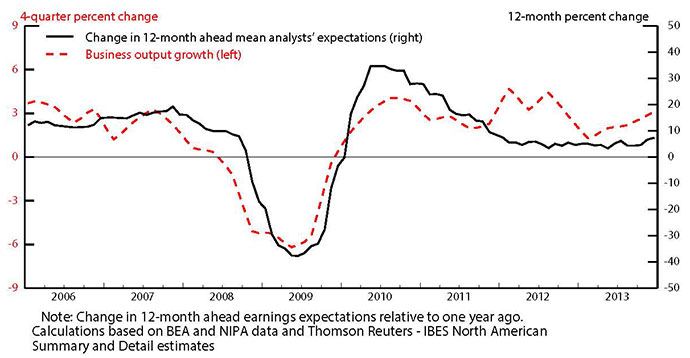
The green portions of the bars represent the part of investment growth not explained by the factors in the model. As noted, these model errors swing from a sizable positive in 2010-11 to a smaller negative in 2012 and close to zero in 2013. Early in the recovery it seems likely that some investment projects that were delayed during the recession due to tight financing conditions and elevated uncertainty were resumed, boosting investment growth above the model for a year or two. In addition, as shown by the black line in Figure 3, profit expectations, measured here by analyst's earnings expectations 12-months ahead, moved up quite rapidly in 2010 but the increases slowed through 2012, a pattern that was not fully captured by business output growth (the red line), the proxy variable used in the model above.

Perspective 2: A long-run growth model

So far, we have analyzed the recent weakness of investment from the point of view of a partial equilibrium model that is helpful in understanding movements in investment growth at a business-cycle frequency. And that analysis showed that an important reason for sluggish investment growth is the sub-par pace of the overall recovery. However, many high-profile analyses in recent years have focused instead on the level of investment and have reached the conclusion that it is disappointingly low.⁴ While these analyses often focus on total private fixed investment (that is, they include residential investment in the calculations), some focus on business investment, as we do here.

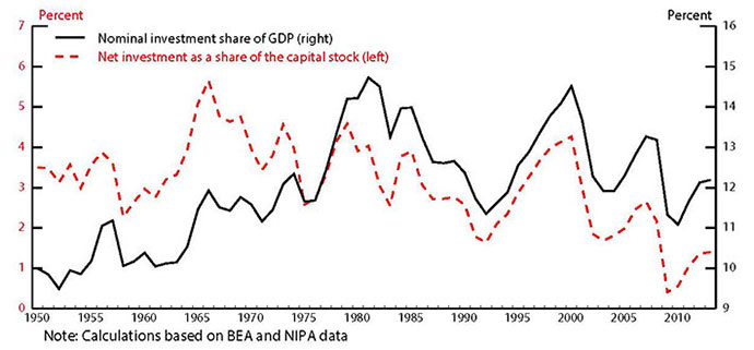
To illustrate this issue we start with two measures that are frequently cited as evidence of the low level of investment. First, the nominal share of gross investment in GDP is shown by the black line in Figure 4. At 12 percent, it is currently in the middle of the 9 - 15 percent range that has prevailed for the past sixty years. However, because the rate of depreciation has been rising over time (as high-tech capital has become increasingly important), the ratio of gross investment to GDP should have an upward trend, suggesting this ratio is pretty low. The red line shows the level of the net investment rate (the growth rate of the capital stock). As noted earlier, this measure is also quite low by historical standards.

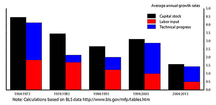
Lower frequency movements of this type can be better explained by looking at the steady-state growth rate in a general equilibrium model--that is, the growth rate of capital that holds when prices have moved to clear the markets for output, labor, and capital, and when the capital stock has completed its transition due to any past shocks. In the Solow growth model, for example, the steady-state net investment rate (the growth rate of the capital stock) is determined by the sum of the growth rate of labor input and the growth rate of technical progress.⁵ Figure 5 shows some suggestive evidence of this simple relationship. Both the rate of net investment and the sum of these two growth rates display a similar slowdown since the 1960s.⁶ In other words, an important reason why businesses are accumulating capital goods at a slower pace than two or three decades ago is likely that the effective labor force that will use that capital (i.e. the labor force adjusted for technical progress that enhances productive efficiency) is also expanding less rapidly.

Concluding thoughts

In this note, we have shown that the recent behavior of investment is not particularly surprising from the perspective of either a standard accelerator-style model or a simple general equilibrium growth model. That said, just like a stopped clock, every model will do well some of the time, and there is still much that we do not understand about the behavior of aggregate investment. For instance, the level of investment currently looks quite low relative to profits or the return on physical capital. In a future post, we plan to address some related issues.

References

Basu, Susantu and John Fernald (2009). "What Do We Know (and Not Know) about Potential Output?" Federal Reserve Bank of St. Louis Review, 91 (4), 187-213.

Elsby, Michael, Bart Hobijn, and Aysegul Sahin (2013). "The Decline of the U.S. Labor Share." Federal Reserve of San Francisco Working Paper Series, 2013-27.

Hall, Robert and Dale Jorgenson (1967). "Tax Policy and Investment Behavior." American Economic Review, 57 (3), 391-414.

Hansen, Lars Peter and Thomas Sargent (1980). "Formulating and Estimating Dynamic Linear Rational Expectations Models." Journal of Economic Dynamics and Control, 2 (1), 7-46.

Jorgenson, Dale (1963). "Capital Theory and Investment Behavior." American Economic Review, 53 (2), 247-259.

Samuelson, Paul (1939). "A Synthesis of the Principle of Acceleration and the Multiplier." Journal of Political Economy, 47 (6), 786-797.

Solow, Robert (1956). "A Contribution to the Theory of Economic Growth." Quarterly Journal of Economics, 70 (1), 65-94.

Tevlin, Stacey and Karl Whelan (2003). "Explaining the Investment Boom of the 1990s." Journal of Money, Credit, and Banking, 35 (1), 2-22.

Whelan, Karl (2003). "A Two-Sector Approach to Modeling U.S. NIPA Data." Journal of Money Credit and Banking, 35 (4), 627-56.

---

1. We thank Tyler Hanson for excellent assistance on this analysis. Return to text

2. The BEA has not yet published capital stock data for 2013. In our analysis we estimate capital stocks using the 2013 investment data, estimates of depreciation rates, and the capital accumulation formula. Return to text

3. We define the user cost of capital according to the standard Hall-Jorgenson rental-rate formula,

where is the relative price of capital, is the real corporate bond rate, is the depreciation rate, is the marginal corporate tax rate, is the investment tax credit, and is the value of tax depreciation allowances. Return to text

4. For example, see "Quantifying the Lasting Harm to the US Economy from the Financial Crisis," draft for the NBER Macro Annual, April 2014, Robert Hall; "The American Investment Drought" WSJ (January 13, 2014); "On Secular Stagnation" Reuters, Lawrence Summers (December 16, 2013); "The Slow Growth of Investment," Econbrowser; Menzie Chin (December 2012); "How to Make Businesses want to Invest Again," New York Times editorial, Greg Mankiw (September 10, 2011). Return to text

5. Solow's (1956) derivation requires constant returns to scale, a constant labor income share, a constant saving rate, and a one-sector model, among other assumptions. Although these restrictions are unlikely to hold (for instance, the labor income share appears to have declined, Elsby et al (2013), and a two-sector growth model may be more realistic, Whelan (2003) and Basu and Fernald (2009)), the Solow model helps set the intuition and we think it is a helpful benchmark. Return to text

6. The growth rate of the labor input is based on BLS data on the civilian population, the labor force participation rate, and the workweek. The growth rate of technical progress is derived from the BLS data on multifactor productivity assuming a Cobb-Douglas production function and a labor share of 2/3. Due to data unavailability, the average growth rate of multifactor productivity includes data only from 2004 to 2012 for the most recent period. Return to text

Please cite as:

Pinto, Eugenio P., and Stacey Tevlin (2014). "Perspectives on the Recent Weakness in Investment," FEDS Notes. Washington: Board of Governors of the Federal Reserve System, May 21, 2014. https://doi.org/10.17016/2380-7172.0018